| Issue |
J. Space Weather Space Clim.
Volume 6, 2016
|
|
|---|---|---|
| Article Number | A11 | |
| Number of page(s) | 7 | |
| DOI | https://doi.org/10.1051/swsc/2016005 | |
| Published online | 22 February 2016 | |
Research Article
Can Open Science save us from a solar-driven monsoon?
Section for Meteorology and Oceanography, Department of Geosciences, University of Oslo, P.O. Box 1022, Blindern, 0315
Oslo, Norway
* Corresponding author: blaken@geo.uio.no
Received:
22
September
2015
Accepted:
26
January
2016
Numerous studies have been published claiming strong solar influences on the Earth’s weather and climate, many of which include documented errors and false-positives, yet are still frequently used to substantiate arguments of global warming denial. Recently, Badruddin & Aslam (2015) reported a highly significant relationship between the Indian monsoon and the cosmic ray flux. They found strong and opposing linear trends in the cosmic ray flux during composites of the strongest and weakest monsoons since 1964, and concluded that this relationship is causal. They further speculated that it could apply across the entire tropical and sub-tropical belt and be of global importance. However, examining the original data reveals the cause of this false-positive: an assumption that the data’s underlying distribution was Gaussian. Instead, due to the manner in which the composite samples were constructed, the correlations were biased towards high values. Incorrect or problematic statistical analyses such as this are typical in the field of solar-terrestrial studies, and consequently false-positives are frequently published. However, the widespread adoption of Open Science approaches, placing an emphasis on reproducible open-source analyses as demonstrated in this work, could remedy the situation.
Key words: Monsoon / Solar Variability / Cosmic ray flux / Statistics
© B.A. Laken, Published by EDP Sciences 2016
 This is an Open Access article distributed under the terms of the Creative Commons Attribution License (http://creativecommons.org/licenses/by/4.0), which permits unrestricted use, distribution, and reproduction in any medium, provided the original work is properly cited.
1. Introduction
Monsoons are planetary-scale circulations that are major features of the tropical atmosphere and the global climate system. Although monsoons in different locations have somewhat different characteristics, monsoon climates are all characterised by a strong seasonal precipitation cycle. Around two-thirds of humanity live within regions influenced by monsoons, and for these people, the onset, intensity and duration of the monsoonal rains are key to their prosperity.
The Indian Summer Monsoon (ISM) is associated with deep convection and rainfall across the northern Indian Ocean and the Indian continent south of around 20 N. The bulk of rainfall migrates from the Indian Ocean region in vernal equinox, to the southern and south-eastern Asian continent and neighbouring ocean regions by northern solstice. It returns northward in autumnal equinox, extending as far as northern Australia in the east, and Madagascar in the west in southern solstice (Clift & Plumb 2008).
Numerous studies have drawn links between variations in solar activity and the intensity of monsoon rainfall based on evidence from palaeoclimatic proxy data (e.g. Neff et al. 2001; Fleitmann et al. 2003; Gupta et al. 2005; Wang et al. 2005; Agnihotri et al. 2011; Tiwari et al. 2015; Xu et al. 2015), from reanalysis data (e.g. Kodera 2004) and from modern observational data (e.g. Mehta & Lau 1997; Bhattacharyya & Narasimha 2005; Maitra et al. 2014; Chaudhuri et al. 2015). However, a mechanism which could account for the reported relationships is unclear, although there are several possibilities: broadly, these mechanisms include so-called top-down solar UV irradiance effects, bottom-up total solar irradiance effects and relationships between atmospheric ionisation from the cosmic ray (CR) flux to aerosols and clouds (Gray et al. 2010).
Recently, a study by Badruddin & Aslam (2015), hereafter BA15, reported a strong link between the solar-modulated CR flux and the ISM. Based on a statistical analysis of observed neutron monitor counts and precipitation records since 1964, they concluded that increases in the CR flux during the ISM resulted in abnormally intense precipitation, while decreases in the CR flux resulted in abnormally weak precipitation. If true, such a relationship would have significant implications for the climate system and importantly be of relevance to the predictability of the ISM. However, as shown in this work, this claim is unsupported by the evidence. As with many solar-terrestrial studies, the numerous pitfalls involved in the statistical analysis of geophysical data led BA15 to produce a false-positive result.
Moreover, of broader interest is a recognition of the large number of fallacious solar-terrestrial studies (e.g. as noted by Pittock 1978, 2009; Farrar 2000; Kristjánsson & Kristiansen 2000; Damon & Laut 2004; Sloan & Wolfendale 2008; Benestad & Schmidt 2009; Čalogović et al. 2010; Laken et al. 2012b; Laken & Čalogović 2013b; Benestad et al. 2015). False-positives within this field are of particular concern, as they contribute to a politically-motivated global warming denial movement, providing material for groups intending to affect policy, such as the Heartland Institute’s Nongovernmental International Panel on Climate Change (NIPCC) or the Centre for the Study of Carbon Dioxide and Global Change (Dunlap & McCright 2010; Benestad et al. 2015). Encouragingly however, a recent shift to open-access, and highly-repeatable workflows offers an opportunity for rapid communal development (and cross-checking) across a broad range of fields, including solar-terrestrial studies: at minimum, such approaches can more effectively facilitate the peer-review process and enhance the quality and reliability of future publications. To illustrate this, this manuscript is supported by an accompanying IPython Notebook (Pérez & Granger 2007), enabling users of the open-source software to easily check, repeat and alter the analysis. This notebook (and all accompanying data) are openly available from figshare (Laken 2015).
2. Data
I have used identical data to the BA15 study: precipitation data over India (source the Indian Institute of Tropical Metrology, Pune, India), and neutron monitor data from Oulu (65.05° N, 25.47° E, 0.8 GV; Usoskin et al. 2001), both monthly means over the period of 1964–2011. A time-series of these data are shown in Figure 1. The strong seasonal precipitation cycle of the monsoon is clearly visible, with the monthly rainfall varying from ~0 mm month−1 during the dry season to ~250 mm month−1 in the wet season. The Oulu neutron monitor data show monthly average counts (min–1) × 103 and span four 11-year solar cycles (beginning with solar cycle 20).
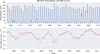 |
Fig. 1. Monthly precipitation (mm) and Olou neutron monitor counts (counts min−1) × 103). |
A precipitation climatology, calculated by compositing the calendar months of the precipitation data, clearly shows the seasonal changes associated with the ISM (Fig. 2). Uncertainty is indicated on the vertical bars in standard error of the mean (SEM), given in Eq. (1), where σ is the sample standard deviation and n is the sample size: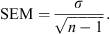 (1)
(1)
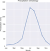 |
Fig. 2. Climatology of monthly precipitation data, with error bars indicating a ±1 standard error of the mean range. |
Subtracting the climatological mean from the precipitation time-series leaves the anomalous (δ) precipitation. This can be used as a measure of how intense or weak the precipitation is for any given month or season, with negative (or positive) values indicating below (or above) average rainfall. This statistic is shown in Figure 3 for means over the months of May–September.
 |
Fig. 3. (a) Mean precipitation anomaly (δ) during the months of May–September, with SEM uncertainty range. The anomaly is calculated by subtracting the precipitation from the climatological mean. (b) Distribution of the anomalies based on a histogram and Gaussian kernel density estimate. |
BA15 ranked the ISM anomalies, isolating the years of the most positive and negative δ precipitation. Their list is given in Table 1. They used these years as the basis for two epoch superposed analysis (composite) samples, to test the hypothesis that variations in the cosmic ray flux (indicated by neutron monitor counts) correspond to these periods of weak and intense ISM precipitation. The composite technique is well suited for such an analysis, as the accumulation and averaging of successive events is useful for isolating low-amplitude signals within data where background variability would otherwise obscure detection (Chree 1913, 1914). However, there are numerous difficulties to effectively use this methodology which must be taken into account so as to arrive at robust conclusions (e.g. as described in Laken & Čalogović 2013a).
Years of strongly negative and positive precipitation anomalies selected by Badruddin & Aslam (2015), which they, respectively, referred to as their Drought and Flood samples.
3. Analysis
3.1. Creating the composites
BA15 examined linear changes in monthly neutron monitor counts, analysed over m = 5 month periods (during the months of May–September) from two samples, each comprised of n = 12 years of monthly-resolution data: i.e. composites from two matrices of n × m elements. The composites – which are vectors of the matrices averaged in the n-dimension – are, respectively, referred to as the “Drought” and “Flood” samples (which I shall also denote here as D and F), and represent the years of weakest and most intense monsoon precipitation, respectively, recorded from 1964 to 2012. These composites are shown in Figure 4, with the May–September periods highlighted.
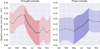 |
Fig. 4. Reproduction of the composite samples of BA15, showing the monthly-resolution pressure-adjusted neutron monitor count rate (units: counts min−1 × 10³) from Oulu station (65.05° N, 25.47° E, 0.8 GV) occurring during 12 years of Indian monsoon “Drought” (D) and “Flood” (F) conditions. Composite means (in the matrix m-dimension) are plotted, with error ranges shown as ±1 standard error of the mean (SEM) value. The period of May–September, selected by BA15 for Pearson’s correlation analysis, has been emphasised in the plots. |
BA15 evaluated the Pearson’s correlation coefficients (r-values) of the means from the D and F samples from May to September and evaluated the statistical significance at the two-tailed probability (p) value (assuming a Gaussian distribution), to test their hypothesis (H1: the CR flux possesses a statistically significant and anti-correlated linear trend during the D and F samples). They obtained values of r = –0.95 (p = 0.01) for D and r = 0.99 (p = 1 × 10⁻³) for F.
At first glance, it is certainly true that these data appear to show a linear change over the highlighted period, anti-correlated between the D and F samples. This is confirmed quantitatively with Pearson’s r correlation analysis and shown to be statistically significant. (As a side point, I note that correlations estimated from data with trends such as these imply a lower effective degree of freedom than the number of data points. If unaccounted for, this will lead to misjudgements in the significance of the correlations.) Before robust conclusions can be drawn from these data however, there are several issues to further examine: firstly, the certainty with which we can know the r-values of the D and F samples given the uncertainty in the data, and secondly, the assumptions regarding the significance tests. I shall now address these issues in turn.
3.2. Uncertainty in the r-values of the composites
As shown in Figure 4, the uncertainty around the composite means is large. It is possible to calculate the r-values that can be obtained within this uncertainty range through re-sampling methods, giving a more comprehensive overview of the possible relationship between the D and F samples and the CR flux data. I have done this by assuming any value within the ±1 SEM range is equally valid, and repeatedly randomly substituting these values and re-calculating Pearson’s r. The result of this procedure is shown in Figure 5. For comparison the r-values of the composite means are marked for both samples. The p-values, from the traditional statistical approach used by BA15 which assumes a Gaussian distribution, are also displayed. Several features are immediately apparent:
-
The results confirm that the D and F samples are skewed towards extreme, and opposing r-values.
-
The realisations cover a large range of r-values, even of opposing sign, particularly in the case of the F sample.
-
Traditional statistical methods show the majority of the correlations do have a low p-value.
-
The re-sampling indicates that the simple mean may have overestimated the r-value of the F sample, as the majority of realisations suggest slightly lower values occurred more frequently.
-
The r-value of the D sample appears more robust, as it coincides with one of the densest portions of its distribution.
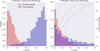 |
Fig. 5. The potential range of r-values of the D (red) and F (blue) samples accounting for uncertainty (left panel). Corresponding p-values from traditional statistical methods assuming a Gaussian distribution are also shown (right panel). Distributions are estimated from Pearson’s r correlations of neutron monitor counts during resamples of the D and F composites, wherein values within the ±1 SEM range were considered equally likely to occur. The r- and p-values from the means of the D and F samples (solid black lines of Fig. 4) are indicated by markers. |
In essence, the D and F samples indeed show opposing trends, which traditional statistical tests confirm to be significant, as BA15 reported. From these results, BA15 concluded that a solar-monsoon link exists and operates via a theoretical CR flux cloud connection. They speculated that this connection impacts the monsoon in the following manner: increases in the CR flux enhance low cloud, rainfall, and surface evaporation, and consequently decrease temperature (and vice versa). They further speculated that their findings may be expanded to the whole tropical and sub-tropical belt, and as a result may impact temperatures at a global scale.
However, while the r-values of the the D and F samples certainly show that a strong, linear change in the CR flux is occurring, I argue that this is neither surprising, nor significant, and ultimately does not support the conclusions of BA15. The main error results from the assumption that the r-values should possess a Gaussian distribution, as I shall demonstrate.
3.3. Monte Carlo simulations of the null hypothesis
The CR flux oscillates as solar activity progresses from minimum to maximum over the course of the ~11-year solar Schwabe cycle. Consequently, by compositing small samples of 5-month periods from a time-series of CR data, as BA15 have done, it is inevitable that the resulting values will regularly show a strongly increasing or decreasing tendency. In other words, the population of r-values, which can be derived from 5-month composites of data dominated by the 11-year solar-cycle, is certain to be ergodic and biased towards extreme values rather than Gaussian.
I demonstrate this using a Monte Carlo (MC) sampling approach, as shown in Figure 6, which shows a normalised histogram calculated from the r-values of 100,000 randomly generated composite samples. Each composite was calculated from matrices of neutron monitor counts of equal dimensions (n × m elements) to the original D and F samples, over May–September periods, randomised in the n-dimension. These data clearly show that the densest parts of the distributions are towards extreme r-values.
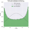 |
Fig. 6. Normalised histogram of r-values drawn from 100,000 Monte Carlo composites representing the null hypothesis (H0). Data are Pearson’s r-values from the Oulu neutron monitor. The histogram has 101 bins over an x-axis range of −1 to 1. For comparison, a normalised Gaussian distribution is plotted on the dashed line: BA15 wrongly assumed the data possessed this distribution. A 4th order polynomial fit to the H0 population is plotted on the solid line: this fit can be used to calculate the density (or probability, p) of a given r-value. |
I note that the May–September restriction is not strictly required, as the CR flux is an external forcing and therefore not related to seasonality. In reality the only requirement is that the MC-samples span an identical time-period as the original samples (5 consecutive months). For more details on the MC method applied to solar-terrestrial studies, including information related to determining optimal size of the simulations, see Laken & Čalogović (2013a).
My statement that the composites are “of equal dimensions to the original” is particularly important, as it alludes to the fact that in order to effectively estimate statistical significance through a MC method, it is necessary to replicate the sample conditions as closely as possible – failure to do so can result in very significant biases in the resulting MC. For example, in this MC the years are random (i.e. the n-dimension described in Sect. 3.1), however, the m dimension is not (i.e. the months of May–September are from the same random n). While seemingly innocuous, such particularities are important: If, for example, both the n and m were random, it would remove temporal autocorrelation from the samples, significantly altering the distribution.
The 4th order polynomial fit, plotted in Figure 6 and given in Eq. (2), follows the MC-generated distribution. The most noticeable disagreement between the fit and the distribution arises at the extreme tails, where the density again begins to decline. A considerably higher order fit (~10th order) is required to capture the behaviour at the extreme tails. However, the approximation from the 4th order polynomial is sufficient to reliably estimate the density of a given histogram bin over the vast majority of the distribution: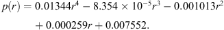 (2)
(2)
Comparing the densities estimated from the 4th order polynomial fit to the Gaussian fit gives the following: for the D sample mean r-value of −0.95, the predicted density in a Gaussian distribution is 0.005, however the polynomial fit estimates the density to be 0.017 (3.7 times greater). For the mean r-value of the F sample, −0.99, the Gaussian estimates a density of 0.004, while the density from the polynomial estimate is 0.020 (4.4 times greater).
In a more general comparison, the extreme tails of the Gaussian distribution covering 5% of its density (in the 0–2.5th and 97.5–100th percentile range) used as a threshold of statistical significance, comparatively relate to 18% of the polynomial density.
Consequently, the high r-values obtained in the BA15 composites do not support a relationship between extremes in Indian precipitation during the monsoon and co-temporal changes in the CR flux, but rather, they are simply among the most commonly obtained values based on BA15’s experimental design.
4. Discussion
The main mechanism suggested to link the CR flux to cloud is via ion-mediated nucleation (Carslaw et al. 2002). The Cosmics Leaving OUtdoor Droplets (CLOUD) experiment at CERN has demonstrated that ion-mediated nucleation may lead to enhancements in aerosol formation of 2–10 times neutral values under specific laboratory conditions – low temperatures characteristic of the upper troposphere, and with low concentrations of amines and organic molecules – however, this effect is absent under conditions more closely representing the lower troposphere (Kirkby et al. 2011; Almeida et al. 2013). Despite this, even if we assume that a significant nucleation of new aerosol particles forms with solar activity, climate model experiments (which include aerosol microphysics schemes) have found that this would still not result in a significant change in either concentrations of cloud condensation nuclei or cloud properties. This is because the majority of the newly formed particles are effectively scavenged by pre-existing larger aerosols (Pierce & Adams 2009; Snow-Kropla et al. 2011; Dunne et al. 2012; Yu et al. 2012). These conclusions are supported by satellite and ground-based observations (e.g. Erlykin et al. 2009; Kulmala et al. 2010; Laken et al. 2012; Benestad 2013; Krissansen-Totton & Davies 2013). For these and additional reasons, the IPCC AR5 concluded that the CR flux has played no significant role in recent global warming (Boucher et al. 2013).
The numerous pitfalls into which solar-terrestrial studies in particular may fall were lucidly outlined decades ago by Pittock (1978, 1979, 1983). More recently, Pittock (2009) also reflected on the main points of these studies in the context of the ability of solar variations to account for any portion of observed climate change. Despite a general awareness of common issues in the field, many studies with improper statistical methods, flawed experimental designs, black-box approaches and ad hoc hypotheses still frequently appear. Consequently, the literature is replete with cases of demonstrated false-positives (Benestad et al. 2015), many of which continue to be used as the basis for global warming denial (e.g. such as in Idso & Singer 2009; Idso et al. 2013), immediately making cases such as the one described in this manuscript in need of address. In this context, Open Science approaches, such as the publication of the code and data accompanying manuscripts (as I have done with this work (Laken 2015), provide a means of ensuring transparency and scientific progress.
Acknowledgments
I would like to thank Dr. Beatriz González-Merino, Dr. Rasmus Benestad (Meteorologisk Institutt), Dr. Jaša Čalogović (University of Zagreb) and Professors Frode Stordal and Joseph H. Lacasce (University of Oslo) and Dr. Eimear Dunne (Finnish Meteorological Institute) for helpful discussions. I also acknowledge the IPython project (http://ipython.org), Continuum Analytics’ Anaconda and the Seaborn library. Data sources: Prof. Ilya Usoskin and the Sodankylä Geophysical Observatory for the Oulu neutron monitor data (http://cosmicrays.oulu.fi), and the Indian Institute of Tropical Meteorology (www.tropmet.res.in) for the monthly precipitation data (which, in this work, were taken directly from BA15). The editor thanks R.E. Benestad and an anonymous referee for their assistance in evaluating this paper.
References
- Agnihotri, R., K. Dutta, and W. Soon. Temporal derivative of Total Solar Irradiance and anomalous Indian summer monsoon: An empirical evidence for a Sun-climate connection. J. Atmos. Sol. Terr. Phys., 73 (13), 1980–1987, 2011. [CrossRef] [Google Scholar]
- Almeida, J., S. Schobesberger, A. Kürten, I.K. Ortega, and O. Kupiainen-Määttä, et al. Molecular understanding of sulphuric acid-amine particle nucleation in the atmosphere. Nature, 502 (7471), 359–363, 2013. [CrossRef] [PubMed] [Google Scholar]
- Badruddin, and O. Aslam. Influence of cosmic-ray variability on the monsoon rainfall and temperature. J. Atmos. Sol. Terr. Phys., 122, 86–96, 2015, DOI: 10.1016/j.jastp.2014.11.005. [CrossRef] [Google Scholar]
- Benestad, R., and G. Schmidt. Solar trends and global warming. J. Geophys. Res.: Atmos., 114 (D14), D14101, 2009. [Google Scholar]
- Benestad, R.E.. Are there persistent physical atmospheric responses to galactic cosmic rays? Environ. Res. Lett., 8 (3), 035049, 2013, DOI: 10.1088/1748-9326/8/3/035049. [CrossRef] [Google Scholar]
- Benestad, R.E., D. Nuccitelli, S. Lewandowsky, K. Hayhoe, H.O. Hygen, R. van Dorland, and J. Cook. Learning from mistakes in climate research. Theor. Appl. Climatol., 1–5, 2015, DOI: 10.1007/s00704-015-1597-5. [Google Scholar]
- Bhattacharyya, S., and R. Narasimha. Possible association between Indian monsoon rainfall and solar activity. Geophys. Res. Lett., 32 (5), L05813, 2005, DOI: 10.1029/2004GL021044. [Google Scholar]
- Boucher, O., D. Randall, P. Artaxo, C. Bretherton, G. Feingold, et al. Clouds and aerosols. Climate change 2013: The physical science basis. Contribution of working group I to the fifth assessment report of the intergovernmental panel on climate change, Cambridge University Press, Cambridge, pp. 571–657, 2013. [Google Scholar]
- Čalogović, J., C. Albert, F. Arnold, J. Beer, L. Desorgher, and E. Flueckiger. Sudden cosmic ray decreases: no change of global cloud cover. Geophys. Res. Lett., 37 (3), L03802, 2010, DOI: 10.1029/2009GL041327. [Google Scholar]
- Carslaw, K., R. Harrison, and J. Kirkby. Cosmic rays, clouds, and climate. Science, 298 (5599), 1732–1737, 2002. [CrossRef] [Google Scholar]
- Chaudhuri, S., J. Pal, and S. Guhathakurta. The influence of galactic cosmic ray on all India annual rainfall and temperature. Adv. Space Res., 55 (4), 1158–1167, 2015. [CrossRef] [Google Scholar]
- Chree, C. Some phenomena of sunspots and of terrestrial magnetism at Kew Observatory. Philos. Trans. R. Soc. London, Ser. A. Containing Papers of a Mathematical or Physical Character, 212, 75–116, 1913. [Google Scholar]
- Chree, C. Some phenomena of sunspots and of terrestrial magnetism. Part II. Philos. Trans. R. Soc. London, Ser. A. Containing Papers of a Mathematical or Physical Character, 245–277, 1914. [Google Scholar]
- Clift, P.D., and R.A. Plumb. The Asian monsoon: causes, history and effects. Vol. 288, Cambridge University Press, Cambridge, 2008. [CrossRef] [Google Scholar]
- Damon, P.E., and P. Laut. Pattern of strange errors plagues solar activity and terrestrial climate data. EOS, Transactions American Geophysical Union, 85 (39), 370–374, 2004. [CrossRef] [Google Scholar]
- Dunlap, R.E., and A.M. McCright. Climate change denial sources, actors and strategies. In: C., Lever-Tracy, Editor. Routledge handbook of climate change and society, Routledge, Abingdon, UK, pp. 240–259, 2010. [Google Scholar]
- Dunne, E., L. Lee, C. Reddington, and K. Carslaw. No statistically significant effect of a short-term decrease in the nucleation rate on atmospheric aerosols. Atmos. Chem. Phys., 12 (23), 11573–11587, 2012. [CrossRef] [Google Scholar]
- Erlykin, A., G. Gyalai, K. Kudela, T. Sloan, and A. Wolfendale. Some aspects of ionization and the cloud cover, cosmic ray correlation problem. J. Atmos. Sol. Terr. Phys., 71 (8), 823–829, 2009. [CrossRef] [Google Scholar]
- Farrar, P.D. Are cosmic rays influencing oceanic cloud coverage – or Is it only El Niño? Clim. Change, 47 (1–2), 7–15, 2000. [CrossRef] [Google Scholar]
- Fleitmann, D., S.J. Burns, M. Mudelsee, U. Neff, J. Kramers, A. Mangini, and A. Matter. Holocene forcing of the Indian monsoon recorded in a stalagmite from southern Oman. Science, 300 (5626), 1737–1739, 2003. [CrossRef] [Google Scholar]
- Gray, L.J., J. Beer, M. Geller, J.D. Haigh, M. Lockwood, et al. Solar influences on climate. Rev. Geophys., 48 (4), 8755–1209, 2010. [CrossRef] [Google Scholar]
- Gupta, A.K., M. Das, and D.M. Anderson. Solar influence on the Indian summer monsoon during the Holocene. Geophys. Res. Lett., 32 (17), 17703–17703, 2005, DOI: 10.1029/2005GL022685. [CrossRef] [Google Scholar]
- Idso, C.D., and S.F. Singer. Climate change reconsidered: 2009 report of the Nongovernmental International Panel on Climate Change (NIPCC). Nongovernmental International Panel on Climate Change, 2009. [Google Scholar]
- Idso, C.D., R.M. Carter, and S.F. Singer. Climate change reconsidered. II: Physical Science, The Heartland Institute, Chicago, Illinois, USA, 2013. [Google Scholar]
- Kirkby, J., J. Curtius, J. Almeida, E. Dunne, J. Duplissy, et al. Role of sulphuric acid, ammonia and galactic cosmic rays in atmospheric aerosol nucleation. Nature, 476 (7361), 429–433, 2011. [CrossRef] [Google Scholar]
- Kodera, K. Solar influence on the Indian Ocean Monsoon through dynamical processes. Geophys. Res. Lett., 31 (24), L24209, 2004, DOI: 10.1029/2004GL020928. [Google Scholar]
- Krissansen-Totton, J., and R. Davies. Investigation of cosmic ray – cloud connections using MISR. Geophys. Res. Lett., 40 (19), 5240–5245, 2013. [CrossRef] [Google Scholar]
- Kristjánsson, J.E., and J. Kristiansen. Is there a cosmic ray signal in recent variations in global cloudiness and cloud radiative forcing? J. Geophys. Res.: Atmos., 105 (D9), 11851–11863, 2000. [CrossRef] [Google Scholar]
- Kulmala, M., I. Riipinen, T. Nieminen, M. Hulkkonen, L. Sogacheva, et al. Atmospheric data over a solar cycle: no connection between galactic cosmic rays and new particle formation. Atmos. Chem. Phys., 10 (4), 1885–1898, 2010. [CrossRef] [Google Scholar]
- Laken, B., E. Pallé, and H. Miyahara. A decade of the moderate resolution imaging spectroradiometer: Is a solar-cloud link detectable? J. Clim., 25 (13), 4430–4440, 2012, DOI: 10.1175/JCLI-D-11-00306.1. [CrossRef] [Google Scholar]
- Laken, B.A. The cosmic ray flux and the Indian Summer Monsoon, figshare, 2015, DOI: 10.6084/m9.figshare.1299413. [Google Scholar]
- Laken, B.A., and J. Čalogović. Composite analysis with Monte Carlo methods: an example with cosmic rays and clouds. J. Space Weather Space Clim., 3, A29, 2013a, DOI: 10.1051/swsc/2013051. [CrossRef] [EDP Sciences] [Google Scholar]
- Laken, B.A., and J. Čalogović. Does the diurnal temperature range respond to changes in the cosmic ray flux? Environ. Res. Lett., 8 (4), 045018, 2013b, DOI: 10.1088/1748-9326/8/4/045018. [CrossRef] [Google Scholar]
- Laken, B.A., E. Pallé, J. Čalogović, and E.M. Dunne. A cosmic ray-climate link and cloud observations. J. Space Weather Space Clim., 2, A18, 2012. [CrossRef] [EDP Sciences] [Google Scholar]
- Maitra, A., U. Saha, and A. Adhikari. Solar control on the cloud liquid water content and integrated water vapor associated with monsoon rainfall over India. J. Atmos. Sol. Terr. Phys., 121, 157–167, 2014. [CrossRef] [Google Scholar]
- Mehta, V.M., and K.-M. Lau. Influence of solar irradiance on the Indian Monsoon-ENSO relationship at decadal-multidecadal time scales. Geophys. Res. Lett., 24 (2), 159–162, 1997. [CrossRef] [Google Scholar]
- Neff, U., S. Burns, A. Mangini, M. Mudelsee, D. Fleitmann, and A. Matter. Strong coherence between solar variability and the monsoon in Oman between 9 and 6 kyr ago. Nature, 411 (6835), 290–293, 2001. [CrossRef] [Google Scholar]
- Pérez, F., and B.E. Granger. IPython: a system for interactive scientific computing. Computing in Science and Engineering, 9 (3), 21–29, 2007, DOI: 10.1109/MCSE.2007.53, URL: http://ipython.org. [Google Scholar]
- Pierce, J., and P. Adams. Can cosmic rays affect cloud condensation nuclei by altering new particle formation rates? Geophys. Res. Lett., 36 (9), L09820, 2009, DOI: 10.1029/2009GL037946. [CrossRef] [Google Scholar]
- Pittock, A.B. A critical look at long-term Sun-weather relationships. Rev. Geophys., 16 (3), 400–420, 1978. [CrossRef] [Google Scholar]
- Pittock, A.B. Solar cycles and the weather: Successful experiments in autosuggestion? Solar-Terrestrial Influences on Weather and Climate, Proceedings of a Symposium/Workshop held at the Fawcett Center for Tomorrow, The Ohio State University, Columbus, Ohio, Springer, pp. 181–191, 1979. [CrossRef] [Google Scholar]
- Pittock, A.B. Solar variability, weather and climate: an update. Quarterly Journal of the Royal Meteorological Society, 109 (459), 23–55, 1983. [CrossRef] [Google Scholar]
- Pittock, A.B. Can solar variations explain variations in the Earth’s climate? Clim. Change, 96 (4), 483–487, 2009. [CrossRef] [Google Scholar]
- Sloan, T., and A.W. Wolfendale. Testing the proposed causal link between cosmic rays and cloud cover. Environ. Res. Lett., 3 (2), 024001, 2008, DOI: 10.1088/1748-9326/3/2/024001. [CrossRef] [Google Scholar]
- Snow-Kropla, E., J. Pierce, D. Westervelt, and W. Trivitayanurak. Cosmic rays, aerosol formation and cloud condensation nuclei: sensitivities to model uncertainties. Atmos. Chem. Phys., 11 (8), 4001–4013, 2011. [CrossRef] [Google Scholar]
- Tiwari, M., S.S. Nagoji, and R.S. Ganeshram. Multi-centennial scale SST and Indian summer monsoon precipitation variability since mid-Holocene and its nonlinear response to solar activity. The Holocene, 2015, 0959683615585840. [Google Scholar]
- Usoskin, I.G., K. Mursula, and J. Kangas. On-line database of cosmic ray intensities. International Cosmic Ray Conference, 9, 3842–3842, 2001. [Google Scholar]
- Wang, Y., H. Cheng, R.L. Edwards, Y. He, X. Kong, Z. An, J. Wu, M.J. Kelly, C.A. Dykoski, and X. Li. The Holocene Asian monsoon: links to solar changes and North Atlantic climate. Science, 308 (5723), 854–857, 2005. [CrossRef] [Google Scholar]
- Xu, H., K.M. Yeager, J. Lan, B. Liu, E. Sheng, and X. Zhou. Abrupt Holocene Indian summer monsoon failures: a primary response to solar activity? The Holocene, 677–685, 2015, DOI: 10.1177/0959683614566252. [CrossRef] [Google Scholar]
- Yu, F., G. Luo, X. Liu, R.C. Easter, X. Ma, and S.J. Ghan. Indirect radiative forcing by ion-mediated nucleation of aerosol. Atmos. Chem. Phys., 12 (23), 11451–11463, 2012, DOI: 10.5194/acp-12-11451-2012. [CrossRef] [Google Scholar]
Cite this article as: Laken BA. Can Open Science save us from a solar-driven monsoon? J. Space Weather Space Clim., 6, A11, 2016, DOI: 10.1051/swsc/2016005.
All Tables
Years of strongly negative and positive precipitation anomalies selected by Badruddin & Aslam (2015), which they, respectively, referred to as their Drought and Flood samples.
All Figures
|
Fig. 1. Monthly precipitation (mm) and Olou neutron monitor counts (counts min−1) × 103). |
| In the text | |
|
Fig. 2. Climatology of monthly precipitation data, with error bars indicating a ±1 standard error of the mean range. |
| In the text | |
|
Fig. 3. (a) Mean precipitation anomaly (δ) during the months of May–September, with SEM uncertainty range. The anomaly is calculated by subtracting the precipitation from the climatological mean. (b) Distribution of the anomalies based on a histogram and Gaussian kernel density estimate. |
| In the text | |
|
Fig. 4. Reproduction of the composite samples of BA15, showing the monthly-resolution pressure-adjusted neutron monitor count rate (units: counts min−1 × 10³) from Oulu station (65.05° N, 25.47° E, 0.8 GV) occurring during 12 years of Indian monsoon “Drought” (D) and “Flood” (F) conditions. Composite means (in the matrix m-dimension) are plotted, with error ranges shown as ±1 standard error of the mean (SEM) value. The period of May–September, selected by BA15 for Pearson’s correlation analysis, has been emphasised in the plots. |
| In the text | |
|
Fig. 5. The potential range of r-values of the D (red) and F (blue) samples accounting for uncertainty (left panel). Corresponding p-values from traditional statistical methods assuming a Gaussian distribution are also shown (right panel). Distributions are estimated from Pearson’s r correlations of neutron monitor counts during resamples of the D and F composites, wherein values within the ±1 SEM range were considered equally likely to occur. The r- and p-values from the means of the D and F samples (solid black lines of Fig. 4) are indicated by markers. |
| In the text | |
|
Fig. 6. Normalised histogram of r-values drawn from 100,000 Monte Carlo composites representing the null hypothesis (H0). Data are Pearson’s r-values from the Oulu neutron monitor. The histogram has 101 bins over an x-axis range of −1 to 1. For comparison, a normalised Gaussian distribution is plotted on the dashed line: BA15 wrongly assumed the data possessed this distribution. A 4th order polynomial fit to the H0 population is plotted on the solid line: this fit can be used to calculate the density (or probability, p) of a given r-value. |
| In the text | |
Current usage metrics show cumulative count of Article Views (full-text article views including HTML views, PDF and ePub downloads, according to the available data) and Abstracts Views on Vision4Press platform.
Data correspond to usage on the plateform after 2015. The current usage metrics is available 48-96 hours after online publication and is updated daily on week days.
Initial download of the metrics may take a while.