| Issue |
J. Space Weather Space Clim.
Volume 3, 2013
|
|
|---|---|---|
| Article Number | A16 | |
| Number of page(s) | 6 | |
| DOI | https://doi.org/10.1051/swsc/2013040 | |
| Published online | 15 April 2013 | |
Research Article
Directional sensitivity of MuSTAnG muon telescope
1
Institute of Physics, University of Greifswald, 17487 Greifswald, Germany
2
Cosmic Ray Division, Yerevan Physics Institute, Yerevan 0036, Armenia
* Corresponding author: e-mail: This email address is being protected from spambots. You need JavaScript enabled to view it.
Received:
26
November
2012
Accepted:
1
April
2013
Abstract
We investigate directional sensitivity of MuSTAnG muon telescope by deriving the distribution of secondary muons, which create the counting rate of telescope, by asymptotic directions of primary protons. This distribution, defined as “directivity function”, allows us to clarify protons appearing from which direction essentially contribute to counting rate of detector. Directivity function has different behavior for the muons falling on the telescope at different zenith and polar angles. Vertical, West, and East fluxes exhibit strong maximums near the asymptotic longitude about 61°, whereas North and South fluxes have larger spread distributions. About 65% of muons, which create the Vertical counting rate of MuSTAnG, are produced by the primary protons, coming in the interval of asymptotic longitudes about (50°, 80°). Using directivity function will allow one to more correctly determine the location of interplanetary disturbances. Analogous analysis, made for other muon detectors, will clarify their directional sensitivities, improving by this the forecasting capability of network of ground-based muon detectors.
Key words: space weather / coronal mass ejection (CME) / magnetosphere / cosmic ray / monitoring
© G. Karapetyan et al., Published by EDP Sciences 2013
 This is an Open Access article distributed under the terms of the Creative Commons Attribution License (http://creativecommons.org/licenses/by/2.0), which permits unrestricted use, distribution, and reproduction in any medium, provided the original work is properly cited.
1. Introduction
The primary cosmic rays reach the Earth after travelling through heliosphere. In times of CME propagation, the flux of cosmic rays is changed due to reflection from CME shock and magnetic clouds. It can lead to the change of proton flux near the Earth, consequently changing the flux of secondary muons in earth atmosphere. As a result, the counting rate of muon detector can vary depending on the presence of CME shocks and magnetic clouds. This phenomenon is a base for forecasting the arrival of CME shocks by monitoring counting rates of several muon detectors, located at different sites around the world (Munakata et al. 2000, 2001; Jansen et al. 2001; Leerungnavarat et al. 2003; Jansen & Behrens 2008). These muon detectors create a global network of multidirectional muon detectors located at Nagoya (Japan), Hobart (Australia), and Sao Martinho (Brazil) and Greifswald (Germany). In this paper we investigate directional properties of Muon Spaceweather Telescope for Anisotropies Greifswald (MuSTAnG), located at the University of Greifswald.
At sea level the flux of secondary particles with energies >150 MeV consists mainly of muons. These muons are created via decay of pions, produced by the interaction of primary protons with air nuclei at the altitudes ~15–20 km. Since the muons lose energy on ionization of air atoms while propagating through the atmosphere, the counting rate of MuSTAnG is created by the muons with threshold energy (at production) of about 2.3 GeV.
For effective forecasting one needs to know from what direction outside of Earth magnetosphere have arrived primary protons, which are responsible for the counting rate of detector. Since Earth magnetic field declines the trajectory of protons, the direction of proton entering the magnetosphere is not coincident with the direction along which this proton falls on the top of atmosphere. The smaller is energy of proton the larger is the difference between these two directions.
For space science applications, one needs to know the direction of protons entering the magnetosphere – the asymptotic direction which is defined by asymptotic longitude A and asymptotic latitude B. The standard analysis of asymptotic directions includes a relationship between the asymptotic direction and the kinetic energy E of primary protons as functions A(E) and B(E). These functions can be derived by using computation code PLANETOCOSMICS (http://cosray.unibe.ch/~laurent/planetocosmics). However, this analysis is not sufficient to clarify the directions from where the main flux of protons comes.
Indeed, consider e.g., asymptotic directions of primary protons, which fall vertically on the top of atmosphere at Greifswald location (geographical coordinates 13°23′ E, 54°05′ N, cutoff energy ~2.5 GeV for the vertical view direction). By getting the functions A(E) and B(E) from PLANETOCOSMICS one obtains the curve, presented in Figure 1.
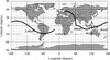 |
Fig. 1. Asymptotic directions (the solid line) of primary protons, falling vertically on the top of atmosphere above Greifswald location (open circle). |
It is seen that protons with energy about 400 GeV come from direction in infinity close to vertical, however ~20 GeV protons decline in Earth magnetosphere on the angle about 45°, coming from asymptotic longitude about 60°. Protons with the energy about 3 GeV decline larger, coming from the direction with asymptotic longitude about 170°, then asymptotic longitude for the 2.4 GeV protons is about – 120° and so on. All of these protons contribute to the vertical counting rate of MuSTAnG. However, this consideration does not clarify what protons give more contribution and what – less. Consequently it is difficult to locate the direction of primary protons, responsible for major part of counting rate. Thus analysis of asymptotic curves as presented in Figure 1 is not sufficient for determining the directions from where coming protons considerably contribute to counting rate of detector. For more advanced analysis one needs to know the distribution of protons, falling on the top of atmosphere by their asymptotic directions. The problem in such a form was first considered in McCracken (1962), Rao et al (1963), and then in Karapetyan (2010) for determining the acceptance cone of neutron monitors. The acceptance cone of a detector is the solid angle containing the asymptotic directions of approach of cosmic ray particles that significantly contribute to the counting rate of the detector (McCracken 1962).
In the present paper we consider this problem for muon detectors and derive the distribution of counting rate of detector by asymptotic directions of primary protons. This distribution, which is called below “directivity function”, is a weighty characteristic of detector, determining its acceptance cone. The width and direction of acceptance cone of detector can be used in determination of the location of CME shock. If the acceptance cone of detector is narrow, then it can be used as well in studies of anisotropies, solar and sidereal variations.
2. The MuSTAnG muon telescope
The MuSTAnG is a multidirectional muon telescope. Figure 2 represents the schematic diagram of the MuSTAnG.
 |
Fig. 2. Schematic diagram of MuSTAnG. μ indicates an incident muon. 1 is an upper detector level, 2 lead layer, 3 lower detector level. |
The muon telescope consists of upper detector layer (1 in Fig. 2), a lead layer of 5.1 cm thickness (2), and a lower detector layer (3). The distance between upper and lower detector layers is 0.95 m. Every detector layer contains 4 × 4 = 16 detectors of 0.25 cm2 area. Thus the telescope contains 32 detectors in total and has full detection area of 4 m2. Detectors are arranged in detector units containing four detectors each. Inside of each detector unit there are located four scintillator plates of 5 cm thickness and 0.25 cm2 area. The scintillator plates are coupled via 1 mm diameter wavelength-shifting optical fibers to photomultiplier modules. Output pulses from the photo multiplier are discriminated and after suitable pulse-shaping, fed into the coincidence electronics. Thus the system comprises two layers each with 16 scintillators operating in between appropriate pairs. The directional information is derived from passage of muons through two, one upper and one lower, detectors. As a result the 1-min count rate data measured in the vertical and four inclined view directions North, East, South, and West (Hippler et al. 2008). In the paper it is investigated how the count rates in these view directions are sensitive to asymptotic directions of primary protons.
3. Directivity function of muon detector
First we obtain the distribution by asymptotic directions of primary protons, falling on the top of atmosphere. Consider this distribution by asymptotic longitude A. The flux of primary protons is described by the known power-law spectral function W(E) ~ (30 GeV/E)2.71/(m2 s sr GeV), where unit of energy is GeV, and the dependence of asymptotic longitude A from the energy – function A(E) is derived from PLANETOCOSMICS code.
By using the equality (1)the searched distribution by asymptotic longitude is determined by the function Dp(A), written as the following
 (2)
(2)
Thus, while the spectral function W(E) represents the flux of protons versus their energy, the directivity function Dp(A) represents the same flux of proton versus their asymptotic longitude. It shows the contribution of primary protons coming from different asymptotic longitudes in the flux, falling on the top of atmosphere at the location to which the directivity function applies. Analogously directivity function versus the latitude B can be derived. Since asymptotic directions are spread largely by the longitudes, we will investigate below directivity function versus asymptotic longitudes.
For vertically falling protons above Greifswald the function Dp(A) is shown in Figure 3, where we see a sharp maximum at the longitude A = 61.1°.
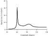 |
Fig. 3. Distribution of primary protons, falling vertically on the top of atmosphere above Greifswald by asymptotic longitudes. |
Thus the derived distribution Dp(A) reveals the presence of an asymptotic direction, from where incoming protons comprise a significant portion of the total flux of protons. However, Dp(A) does not yet clarify the main problem: the distribution of the counting rate by the longitude A of primary protons. Since counting rate is created by the secondary muons, produced in atmosphere, the equivalent problem is the distribution of secondary muons by the longitude of primary protons. To solve this problem we will introduce a directivity function for secondary muons similar to (2) by replacement of the flux of protons W(E) with the flux of muons produced by these protons, e.g., for the vertical view direction with the flux V(E) defined below. Note that while W(E) is differential flux of protons, nevertheless V(E) is not the differential flux of muons. Really, differential flux of muons S(x) is formed by all protons having energy larger than x, i.e., it is presented by the equation (3)where yield function y(E, x) connects the flux of muons S(x), having energy x, with the flux of protons W(E), having energy E.
At E ~ x yield function y(E, x) is negligibly small, therefore the value of integral (3) is determined by large values of E. For these E the dependence of y(E, x) from the energy of muons x can be neglected, assuming that y(E, x) ~ y(E) is the function of only the energy of proton. Then by differentiating (3) it is obtained (4)
(4)
Integrating y(E) in interval (Eth, E) in muon energy, where Eth ~ 2.3 GeV, we obtain total yield function Y(E), then by multiplying it on the proton flux W(E), the searched flux of muons V(E) for substituting in (2) is obtained (5)
(5)
 (6)
(6)
Thus, the function V(E) is the flux of muons with energies (Eth … E), produced by the flux of protons W(E). Functions y(E), Y(E), W(E), S(E), and V(E), calculated by (4)–(6), are presented in Figure 4. For S(E) we prepared the function 8000E/(E + 3)4.21/(m2 s sr GeV) (where unit of energy is GeV), which in the energy range from ~1 GeV to several hundred GeVs well interpolates experimental data, presented in (Bellotti et al 1999; Hebbeker & Timmermans 2002; Yoshida et al 2006; Hagmann et al 2007).
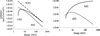 |
Fig. 4. Left panel: Differential spectums of protons W(E) (the dashed line), muons S(E) (the dotted line), and function V(E) (the solid line). Right panel: yield functions y(E) (the dotted line) and Y(E) (the solid line). |
It is seen that at energies <10 GeV the function V(E) considerably decreases comparing with W(E), because of ineffective production of muons by the protons with small energies. Thus substituting the flux of muons V(E) from (6) to (2) instead of the flux of protons W(E) we obtain the directivity function of muons D
m(A) as the following (7)
(7)
Thus while spectral function V(E) gives the distribution of muons by energies, the directivity function Dm(A) gives the distribution of these muons by asymptotic longitudes of primary protons. By integrating V(E) over energies >Eth we will obtain total flux of muons with energy >Eth, the same value is obtained as well by integrating the differential spectrum of muons S(E), i.e., (8)
(8)
Function Dm(A) is shown in Figure 5. Compared to Figure 3 the maximum at the longitude about 61° is seen sharper and values at larger longitudes are reduced more strongly. Such a decrease of muons, produced by the protons coming from larger longitudes, is conditioned by the reduction of function V(E) at smaller energies, since corresponding protons larger decline in magnetosphere. From analysis of function Dm(A) it follows that about 65% of all muons are produced by the protons coming from asymptotic longitudes in the interval (50°, 80°). Corresponding asymptotic latitudes are spread in the interval ~(−10°, 40°). Thus, the vertical flux of secondary muons is highly sensitive to directions of primary protons, depending mainly on the protons coming from asymptotic longitudes in narrow interval ~30° around longitude 61°. These protons create the muons in energy interval ~(6 GeV, 36 GeV), so that (9)
(9)
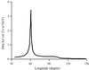 |
Fig. 5. Directivity function of vertical flux of muons, i.e., the distribution of muons, produced by vertically falling protons above Greifswald, by asymptotic longitudes of primary protons. |
Thus the function Dm(A) is the distribution of vertically falling muons by asymptotic longitudes of primary protons, so it represents approximately the longitudinal sensitivity of Vertical count of MuSTAnG.
Analogously one can find the distribution functions of an inclined flux of muons. Consider inclined fluxes of muons, falling on the detector at zenith angle 30° from four different directions: North, East, South, and West. Polar angle ϕ is counted clockwise from North direction, so that these directions have polar angles respectively ϕ = 0, 90°, 180°, and 270°. These fluxes approximately represent directional sensitivity of corresponding inclined channels of MuSTAnG. Getting from PLANETOCOSMICS the functions A(E) corresponding to these zenith and polar angles and calculating directivity functions (7) we obtain the graphs, presented in Figure 6. It is seen that directivity functions for East and West fluxes of muons are approximately akin to that of Vertical flux, presented in Figure 5, whereas the North and South fluxes differ more from Vertical flux.
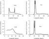 |
Fig. 6. Directivity functions of the inclined (at zenith angle 30°) fluxes of muons. All directivity functions, except of South, are multivalued, that are shown by the dotted curves. The net directivity functions, which are the sum of all branches of multivalued functions, are shown by the solid curves. |
Note that the protons falling on the top of atmosphere at 30° zenith angle have complicated trajectories in magnetosphere, so that protons at different energies and different asymptotic longitudes can arrive at the top of atmosphere with the same zenith and polar angles. It means that the function Dm(A), calculated by (7), can be multivalued in some interval of longitudes. In such cases all its branches should be summed to obtain real distribution function of muons.
Thus these directivity functions qualitatively represent directional sensitivity of North, East, South, and West counts of MuSTAnG. Based on these functions one can conclude that the most directional sensitivity have Vertical, East, and West counts, whereas the North and South counts are less sensitive to the asymptotic directions of primary protons. Therefore for accurate measurements one can use the sum of Vertical, East, and West counting rates. In Figure 7 there is presented cross-section of acceptance cone for Vertical count of MuSTAnG, inside which coming protons create about 65% of counting rate. Such presentation of directional sensitivity of detector by locating on the map appropriate area of cross-section of acceptance cone is more informative instead of usually used curves of asymptotic directions.
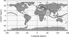 |
Fig. 7. The cross-section of the acceptance cone for vertical count of MuSTAnG, inside which incoming protons create about 65% of counting rate. The solid curve is asymptotic directions of vertical flux of protons. |
4. Conclusions
We investigated directional sensitivity of MuSTAnG muon telescope by deriving the distribution of counting rate by asymptotic directions of primary protons. This distribution, called directivity function, determines the acceptance cone of detector, showing protons appearing from which direction significantly contribute to counting rate. As a result the directional sensitivity of detector is shown on the map as the area of cross-section of acceptance cone. We have shown that a large contribution to counting rate is generated by protons, coming at narrow interval of longitudes ~(50°, 80°) and corresponding energies ~(36 GeV, 6 GeV). The most sensitive measurements are the Vertical, East, and West counts of MuSTAnG, so that for accurate analysis the sum of these three counting rates should be used. The narrow directivity function of MuSTAnG will allow us to determine the location of CME shock more accurately, improving forecasting capability of the telescope. The method developed in this paper can be used for calculating directional sensitivity of other muon detectors, to clarify whether or not their counting rates are also sensitive to asymptotic directions of primary protons. Muon detectors with narrow acceptance cones can be used as well for investigation of anisotropy of galactic cosmic rays by processing hourly counts, collected during several years.
Acknowledgments
The work was supported by the European Space Agency (ESA) and the Deutscher Akademischer Austauschdienst (DAAD). G.K. thanks DAAD for providing the opportunity for a research stay at the University of Greifswald.
References
- Bellotti, R., F. Cafagna, M. Circella, and C.N. De Marzo, Balloon measurements of cosmicray muon spectra in the atmosphere along with those of primary protons and helium nuclei over mid-latitude, Phys. Rev. D, 60, 052002, 1999. [NASA ADS] [CrossRef] [Google Scholar]
- Hagmann, C., D. Lange, and D. Wright, Monte Carlo Simulation of Proton-induced Cosmic-Ray Cascades in the Atmosphere, Lawrence Livermore National Laboratory, UCRL-TR, 2007. [CrossRef] [Google Scholar]
- Hebbeker, T., and C. Timmermans, A compilation of high energy atmospheric muon data at sea level, Astropart. Phys., 18, 107–127, 2002. [CrossRef] [Google Scholar]
- Hippler, R., A. Mengel, F. Jansen G. Bartling, W. Göhler, et al., First spaceweather observations at MuSTAnG – the muon spaceweather telescome for anisotropies at Greifswald, Proc. of 30th International Cosmic Ray Conference, Mexico, 1, pp. 347–350, 2008. [Google Scholar]
- Jansen, F., K. Munakata, M.L. Duldig, and R. Hippler, Muon detectors – the real-time, ground based forecast of geomagnetic storms in Europe, ESA Space Weather Workshop, December, 2001. [Google Scholar]
- Jansen, F., and J. Behrens, Cosmic rays and space situational awareness in Europe, 21st European Cosmic Ray Symposium in Kosice, Slovakia, pp. 626–632, 2008. [Google Scholar]
- McCracken, K.G., The cosmic-ray flare effect: 1. Some new methods of analysis, J. Geophys. Res., 67, 423, DOI: 10.1029/JZ067i002p00423, 1962. [CrossRef] [Google Scholar]
- Karapetyan, G.G., Investigation of cosmic ray anisotropy based on Tsumeb neutron monitor data, Astropart. Phys., 33, 146–150, 2010. [CrossRef] [Google Scholar]
- Leerungnavarat, K., D. Ruffolo, and J.W. Bieber, Loss cone precursors to Forbush decreases and advance warning of space effects, Astrophys. J., 593, 587–596, 2003. [CrossRef] [Google Scholar]
- Munakata, K., J. Bieber, Y. Shin-ichi, C. Kato, M. Koyama, et al., Precursors of geomagnetic storms observed by the muon detector network, J. Geophys. Res., 105, 27457–27468, 2000. [CrossRef] [Google Scholar]
- Munakata, K., J. Bieber, J.W. Kuwabara, T. Hattori, K. Inoue, et al., A prototype muon detector network, covering a full range of cosmic ray pitch angles, Proc. 27th International Cosmic Ray Conference, Hamburg, 9, 3494–3497, 2001. [Google Scholar]
- Rao, U.R., K.G. McCracken, and D. Venkatesan, Asymptotic cones of acceptance and their use in the study of the daily variation of cosmic radiation, J. Geophys. Res., 68, 345–369, 1963. [NASA ADS] [CrossRef] [Google Scholar]
- Yoshida, K., R. Ohmori, Y. Sato, T. Kobayashi, Y. Komori, et al., Cosmic-ray spectra of primary protons and high altitude muons deconvolved from observed atmospheric gamma rays, Phys. Rev. D, 74, 083511, http://cosray.unibe.ch/~laurent/planetocosmics, 2006. [CrossRef] [Google Scholar]
Cite this article as: Karapetyan G, Ganeva M & Hippler R: Directional sensitivity of MuSTAnG muon telescope. J. Space Weather Space Clim., 2013, 3, A16.
All Figures
|
Fig. 1. Asymptotic directions (the solid line) of primary protons, falling vertically on the top of atmosphere above Greifswald location (open circle). |
| In the text | |
|
Fig. 2. Schematic diagram of MuSTAnG. μ indicates an incident muon. 1 is an upper detector level, 2 lead layer, 3 lower detector level. |
| In the text | |
|
Fig. 3. Distribution of primary protons, falling vertically on the top of atmosphere above Greifswald by asymptotic longitudes. |
| In the text | |
|
Fig. 4. Left panel: Differential spectums of protons W(E) (the dashed line), muons S(E) (the dotted line), and function V(E) (the solid line). Right panel: yield functions y(E) (the dotted line) and Y(E) (the solid line). |
| In the text | |
|
Fig. 5. Directivity function of vertical flux of muons, i.e., the distribution of muons, produced by vertically falling protons above Greifswald, by asymptotic longitudes of primary protons. |
| In the text | |
|
Fig. 6. Directivity functions of the inclined (at zenith angle 30°) fluxes of muons. All directivity functions, except of South, are multivalued, that are shown by the dotted curves. The net directivity functions, which are the sum of all branches of multivalued functions, are shown by the solid curves. |
| In the text | |
|
Fig. 7. The cross-section of the acceptance cone for vertical count of MuSTAnG, inside which incoming protons create about 65% of counting rate. The solid curve is asymptotic directions of vertical flux of protons. |
| In the text | |
Current usage metrics show cumulative count of Article Views (full-text article views including HTML views, PDF and ePub downloads, according to the available data) and Abstracts Views on Vision4Press platform.
Data correspond to usage on the plateform after 2015. The current usage metrics is available 48-96 hours after online publication and is updated daily on week days.
Initial download of the metrics may take a while.