| Issue |
J. Space Weather Space Clim.
Volume 4, 2014
|
|
|---|---|---|
| Article Number | A18 | |
| Number of page(s) | 8 | |
| DOI | https://doi.org/10.1051/swsc/2014016 | |
| Published online | 22 May 2014 | |
Regular Article
The importance of geomagnetic field changes versus rising CO2 levels for long-term change in the upper atmosphere
British Antarctic Survey, High Cross, Madingley Road, Cambridge, CB3 0ET, United Kingdom
* Corresponding author: e-mail: This email address is being protected from spambots. You need JavaScript enabled to view it.
Received:
30
October
2013
Accepted:
7
May
2014
Abstract
The Earth’s upper atmosphere has shown signs of cooling and contraction over the past decades. This is generally attributed to the increasing level of atmospheric CO2, a coolant in the upper atmosphere. However, especially the charged part of the upper atmosphere, the ionosphere, also responds to the Earth’s magnetic field, which has been weakening considerably over the past century, as well as changing in structure. The relative importance of the changing geomagnetic field compared to enhanced CO2 levels for long-term change in the upper atmosphere is still a matter of debate. Here we present a quantitative comparison of the effects of the increase in CO2 concentration and changes in the magnetic field from 1908 to 2008, based on simulations with the Thermosphere-Ionosphere-Electrodynamics General Circulation Model (TIE-GCM). This demonstrates that magnetic field changes contribute at least as much as the increase in CO2 concentration to changes in the height of the maximum electron density in the ionosphere, and much more to changes in the maximum electron density itself and to low-/mid-latitude ionospheric currents. Changes in the magnetic field even contribute to cooling of the thermosphere at ~300 km altitude, although the increase in CO2 concentration is still the dominant factor here. Both processes are roughly equally important for long-term changes in ion temperature.
Key words: space climate / ionosphere / thermosphere / modeling / global change
© I. Cnossen, Published by EDP Sciences 2014
 This is an Open Access article distributed under the terms of the Creative Commons Attribution License (http://creativecommons.org/licenses/by/4.0), which permits unrestricted use, distribution, and reproduction in any medium, provided the original work is properly cited.
1. Introduction
The study of long-term (multi-decadal) changes in the upper atmosphere started with the prediction that a doubling of the CO2 concentration would lead to a ~50 K cooling of the thermosphere at 300–400 km altitude (Roble & Dickinson 1989). The subsequent atmospheric contraction would cause a lowering of ionospheric layers and a decrease in neutral density at fixed height (Rishbeth & Roble 1992), while the maximum electron density of ionospheric layers should not be affected much (Rishbeth 1990; Rishbeth & Roble 1992). Observational evidence has confirmed many of these predictions, at least in a qualitative sense: the global mean neutral density at fixed heights of 250–400 km has been decreasing (Keating et al. 2000; Emmert et al. 2004; Emmert & Picone 2011), the ion temperature, which is closely coupled to the neutral temperature, has been decreasing at several stations (Donaldson et al. 2010; Zhang et al. 2011; Zhang & Holt 2013), and at many stations decreasing trends in the heights of the maximum electron density of the ionospheric E and F2 layers have been found (Bremer 1992, 2008; Ulich & Turunen 1997; Jarvis et al. 1998; Bremer et al. 2012). It has also been suggested that the changes in the ionosphere arising from increased greenhouse gases could be responsible, at least partly, for observed long-term changes in the daily amplitude of magnetic perturbations associated with the solar quiet (Sq) current system flowing in the low- to mid-latitude dayside ionosphere (Torta et al. 2009; Elias et al. 2010).
However, model predictions of the effects of the increase in CO2 concentration that has actually occurred tend to be too weak to explain the trends observed over the past decades fully (Cnossen 2012). There are also inconsistencies between the reported magnitudes of long-term trends in ion temperature and neutral density, which still need to be reconciled (Akmaev 2012). In addition, several ionosonde stations show increases in the height of the peak of the F2 layer, hmF2, rather than the expected decrease (Bremer 1998; Upadhyay & Mahajan 1998), and many stations show significant trends in the critical frequency of the F2 layer, foF2 (Upadhyay & Mahajan 1998; Elias & Ortiz de Adler 2006), which is directly related to the maximum electron density of the F2 layer, NmF2 (NmF2 ∝ (foF2)2). These discrepancies with the predicted effects of enhanced CO2 levels mean that other drivers of long-term change may be important also.
Indeed, Cnossen & Richmond (2008, 2013) showed that changes in the Earth’s main magnetic field can cause changes in the ionosphere of similar magnitude to the effects predicted for the increase in CO2 concentration, and can result in decreases as well as increases (depending on location) in both hmF2 and foF2. The underlying physical mechanisms responsible for these effects were explored through a series of idealized modeling studies and are now quite well understood (Cnossen et al. 2011, 2012; Cnossen & Richmond 2012). Yet, the importance of geomagnetic field changes as a driver of long-term change in the upper atmosphere still appears to be underappreciated. The increase in CO2 concentration generally remains to be thought of as the main driver of long-term changes in the upper atmosphere (e.g., Laštovička et al. 2012), despite the inconsistencies mentioned above.
Here we directly compare some of the effects of the increase in CO2 concentration and changes in the geomagnetic field from 1908 to 2008. Such a direct, quantitative comparison has so far not been done, because different models and different setups have been used to study the effects of enhanced CO2 levels and geomagnetic field changes in the past (e.g., Akmaev et al. 2006; Cnossen & Richmond 2008, 2013; Qian et al. 2009). We address this problem with a series of simulations with the Thermosphere-Ionosphere-Electrodynamics General Circulation Model (TIE-GCM), all set up in the same way. These allow us to quantify the effects of the increase in CO2 concentration and changes in the magnetic field both separately and combined. This helps to establish the relative importance of both drivers in causing long-term trends in the upper atmosphere more precisely and identify any interactions between them. We also estimate the significance of the effects against day-to-day variability, which has not been done before for the effects of changes in CO2 concentration, even though this is essential in determining their importance. The simulations clearly demonstrate that changes in the Earth’s magnetic field can be at least as important as enhanced CO2 levels for long-term change in the upper atmosphere, if not more important, depending on the variable studied.
2. Methods
The TIE-GCM is a time dependent, three-dimensional model that solves the fully coupled, nonlinear, hydrodynamic, thermodynamic, and continuity equations of the thermospheric neutral gas self-consistently with the ion continuity equations. In the setup used here, the model grid consists of 36 latitude and 72 longitude points (5° × 5° resolution) and 29 pressure levels between ~96 km and ~500 km with a spacing of half a scale height. The model is well-established and has been widely used in the thermosphere-ionosphere community, so we will only mention a few important aspects here. More information on the original model setup can be found in Roble et al. (1988) and Richmond et al. (1992). An up-to-date overview of the development of the TIE-GCM and its current state, including some model validation examples, is provided by Qian et al. (2014) and references therein.
The TIE-GCM calculates the electric potential self-consistently at geomagnetic latitudes equatorward of ±60°. At geomagnetic latitudes poleward of ±75° the electric potential was externally imposed using the empirical Heelis et al. (1982) model. In between is a transition zone where the numerical solution is gradually more constrained by the empirical model. The Kp index was used as input to the Heelis et al. (1982) model. The Kp index was also used to parameterize the effects of energetic particle precipitation from the magnetosphere, also done in a geomagnetic coordinate system. Any effects of changes in the geographic locations of the auroral ovals (and the associated phenomena), which would be expected to arise from changes in the geographic locations of the magnetic poles, are therefore accounted for. However, the magnitudes of the high-latitude electric potential and the hemispheric power of precipitating particles are the same for each simulation (but vary over the duration of each simulation according to variations in the Kp index).
At its lower boundary, the TIE-GCM allows for tidal forcing with the Global Scale Wave Model (GSWM). Here, the GSWM migrating diurnal and semi-diurnal tides of Hagan & Forbes (2002, 2003) were used. As the tidal forcing was kept the same for all simulations, any effects of changes in the tides that might arise from changes in the geomagnetic field or (perhaps more likely) from an increase in CO2 concentration are not accounted for.
All our simulations were run for 61 days from 0 UT on 1st March to 0 UT on 1st May with the observed solar and geomagnetic forcing (F10.7 and Kp indices) of the year 2008. On average, the solar activity during this interval was very low (F10.7 ~ 70 solar flux units), and geomagnetic conditions were relatively quiet. The Kp index was never higher than 6, and mostly around 2–3. A subsection of the same interval has been simulated previously by Cnossen & Richmond (2013) with the Coupled Magnetosphere-Ionosphere-Thermosphere (CMIT) model to study the effects of changes in the magnetic field. Here we have chosen to use the TIE-GCM instead, because it runs much faster, allowing for longer simulations, which is needed to establish the statistical significance of differences between simulations more reliably. The downside of this choice is that any changes in solar wind-magnetosphere-ionosphere (SW-M-I) coupling that may arise from changes in the magnetic field are not accounted for. However, Cnossen & Richmond (2012) showed that changes in SW-M-I coupling are mainly important during geomagnetically disturbed conditions; for quiet conditions these should have only minor effects at most.
The control simulation was set up with the CO2 concentration of 2008 (385 ppm) and the magnetic field of 2008, specified by the International Geomagnetic Reference Field (IGRF) (Finlay et al. 2010). We then performed three additional simulations to quantify the effects of the change in CO2 concentration since 1908, the changes in the magnetic field since 1908, and their combined effects, respectively. In the first experimental simulation the CO2 concentration was changed to the level in 1908 (300 ppm) and the lower boundary temperature was increased from 180 K (used in the control experiment) to 182 K to reflect the warming effect of a lower CO2 concentration at ~97 km altitude, following Qian et al. (2009). Everything else was kept as in the control run. We note that it is assumed that the change in the ground-level CO2 concentration (i.e. from 300 ppm in 1908 to 385 ppm in 2008) is representative also of the change in CO2 concentration in the upper atmosphere. In the second experimental simulation, only the magnetic field was changed from the IGRF of 2008 to the IGRF of 1908, with again all other settings the same as in the control run. In the last simulation, we used both the IGRF of 1908 and the CO2 concentration of 1908, again with a lower boundary temperature of 182 K. An overview of these simulation settings is given in Table 1. The four simulations are labeled with a code name, which will be used in the rest of the text and figures for easy reference.
Overview of the simulation settings used.
Magnetic perturbations associated with currents flowing in the ionosphere were calculated with a post-processing code described by Doumbia et al. (2007) and Richmond & Maute (2014). Results are presented for the daily amplitude of these perturbations, calculated as the difference between the maximum and minimum values of the perturbations for a given field component at each location for each day. At low- to mid-latitudes this can be interpreted as the daily amplitude of the solar quiet (Sq) magnetic variation, as the geomagnetic activity level is fairly low throughout the simulation interval. Magnetic perturbations at high latitudes may be less reliable, as these are more influenced by interactions with the magnetosphere, which is not represented in the TIE-GCM. We also note that the TIE-GCM tends to underestimate E region electron densities and conductivities somewhat and therefore also tends to underestimate magnetic perturbations. Any differences in magnetic perturbations between simulations may therefore be underestimated as well. In addition, any effects of currents flowing in the solid earth or oceans and effects of local variations in the subsurface conductivity are not taken into account.
The results are presented in the form of maps of the 61-day mean (or mean difference) of a given variable. Except when daily amplitudes are considered, maps are organized in local time (LT) rather than universal time (UT), so that the results can be more easily compared to observed long-term trends, which are often for a specific local time or local time range. Often noon-time values are chosen. Local time maps were therefore constructed by extracting for each 15° wide longitude sector the data for the UT corresponding to 12 LT and then joining up these longitude sectors to form one map.
At each grid point, a t-test was done to assess the statistical significance of the 61-day mean differences between the experimental simulations and the control run against day-to-day variability, represented by the standard deviation of the 61 values (one for each day) at that grid point. This means that each day was taken as an independent data point, which is reasonable given a typical relaxation time of about 12–15 h in the thermosphere at 350 km (Maeda et al. 1992).
3. Results
3.1. Neutral temperature
Figure 1 shows a map of the 61-day average neutral temperature in the thermosphere at 3.2 × 10⁻⁸ hPa (~300 km) for the control experiment (MC2008; panel a) and the difference with each of the subsequent experiments (panels b–d) at 12 LT. The effect of the increase in CO2 concentration from 1908 to 2008 is, as expected, a fairly uniform decrease in neutral temperature of about 8 K (panel b). However, this effect is only statistically significant at relatively low latitudes. This is due to smaller day-to-day variability in the lower latitude areas. The simulated 61-day standard deviation of the neutral temperature at 12 LT and 3.2 × 10⁻⁸ hPa is about 20 K at low- to mid-latitudes, while at high latitudes this increases to 40 K or more. Any difference between simulations (the signal) therefore stands out more clearly at lower latitudes.
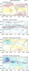 |
Fig. 1. Sixty-one-day mean neutral temperature for the control case (MC2008; panel a) and the difference with C1908, M1908, and MC1908 (panels b–d) at 12 LT at a pressure level of 3.2 × 10⁻⁸ hPa (~300 km). The contour interval for the difference plots is 2 K between −12 and +12 K, with an additional contour at −16 K for the bottom panel. Light (dark) shading indicates statistical significance at the 95% (99%) level. |
Changes in the magnetic field from 1908 to 2008 (panel c) cause the strongest changes in neutral temperature at high magnetic latitudes, i.e. near the near the northern hemisphere (NH) and southern hemisphere (SH) magnetic poles, with a cooling of up to 10 K in the NH and a warming of up to 12 K in the SH. In other areas a more modest warming is found of about 4 K. The overall warming is consistent with the overall decrease in magnetic field strength that has taken place over the past century (Cnossen et al. 2011, 2012), while the more localized changes near the magnetic poles are probably associated with the northward and westward movement of the magnetic poles over the past century, which creates changes in the distribution and amount of Joule heating in the auroral regions (Cnossen & Richmond 2012). However, nearly all of the changes in neutral temperature caused by magnetic field changes are statistically insignificant, except for a small patch of cooling over North America.
Still, when the effects of changes in CO2 concentration and changes in the magnetic field are combined (panel d), the cooling over North America and parts of the Atlantic and Pacific Oceans produced by changes in the magnetic field adds to the cooling caused by the increase in CO2 concentration. This creates a strong, significant cooling over those parts of the world of up to 18 K. Some areas that did not show a significant cooling for either of the two drivers individually, do show a significant change when their effects are added. Conversely, in areas where the effects of changes in the magnetic field oppose the effects of the increase in CO2 concentration (e.g. all eastern longitudes), significant change occurs over smaller areas than found for the increase in CO2 concentration alone. The effects of the two processes thus appear to be more or less additive, indicating that there is not much interaction between them.
3.2. Ion temperature
Figure 2 shows the ion temperature at 3.2 × 10⁻⁸ hPa (~300 km) for the control experiment (MC2008; panel a) and the difference with each of the subsequent experiments (panels b–d) at 12 LT. The increase in CO2 concentration causes a fairly uniform decrease in ion temperature of 6–11 K and is only significant at relatively low latitudes (panel b). This is similar to what we found for the neutral temperature.
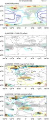 |
Fig. 2. Sixty-one-day mean ion temperature for the control case (MC2008; panel a) and the difference with C1908, M1908, and MC1908 (panels b–d) at 12 LT at a pressure level of 3.2 × 10⁻⁸ hPa (~300 km). Contours for the difference plots are at 0, ±10, ±25, ±50, and ±100 K. Light (dark) shading indicates statistical significance at the 95% (99%) level. |
However, the ion temperature is more significantly affected by changes in the Earth’s magnetic field (panel c) than the neutral temperature is. Significant changes in ion temperature are mainly found over a region bounded by ~80° W–40° E and ~30° S–30° N, which roughly corresponds to a region we have previously referred to as the Atlantic region (Cnossen & Richmond 2013). The changes in ion temperature found here more or less follow the changes in electron temperature (not shown), which are related to changes in electron density (see following section): where the electron density is lower, the same amount of solar energy is distributed over a smaller number of electrons, leading to a higher electron temperature, and vice versa where the electron density is higher (see also Cnossen & Richmond 2013). When the effects of the increase in CO2 concentration and magnetic field changes are combined (panel d), the changes appear again more or less additive, i.e. panel d appears to correspond more or less to the sum of panels b and c.
3.3. F2 layer ionosphere
In the densest part of the ionosphere, the F2 layer, the two key parameters that have shown long-term changes in observational records are the critical frequency, foF2 (directly related to the maximum electron density), and the height of the peak in electron density, hmF2. Their responses to the increase in CO2 concentration and changes in the geomagnetic field over the past century are compared in Figure 3, again for 12 LT.
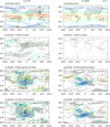 |
Fig. 3. Sixty-one-day mean hmF2 (left) and foF2 (right) for the control case (MC2008; panels a/e) and the difference with C1908, M1908, and MC1908 (panels b/f, c/g, and d/h, respectively) at 12 LT. The contour interval for the hmF2 difference plots is 20 km between −60 and +60 km, with additional contours at −5 and +5 km. The contour interval for the foF2 difference plots is 0.25 MHz between −1.5 and +1.5 MHz. Light (dark) shading indicates statistical significance at the 95% (99%) level. |
The increase in CO2 concentration over the past century (panel b) caused a fairly uniform decrease in hmF2 of about 5 km, but this is not statistically significant everywhere. Significant differences are mainly found in bands between 30° and 50° latitude in both hemispheres. The magnitude of the change agrees quite well with model predictions by Qian et al. (2009), when scaling the results of their simulations, which were for a doubling of the CO2 concentration from a base level of 365 ppm, to the 85 ppm increase from 1908 to 2008 simulated here. There is no noticeable effect of the increase in CO2 concentration on foF2 (panel f). All the changes are smaller than ±0.2 MHz (±2.5%) and are not statistically significant, in agreement with theoretical and previous model predictions (Rishbeth 1990; Rishbeth & Roble 1992).
Changes in the magnetic field between 1908 and 2008 clearly have had a much stronger effect on both hmF2 and foF2 in various parts of the world (panels c and g). The strongest effects, with changes in hmF2 of up to −60 and +40 km and changes in foF2 of up to −1.25 to +0.5 MHz, are found roughly between 40° S–40° N and 80° W–50° E, again roughly corresponding to the Atlantic region mentioned before. Still, considerable significant changes are also found outside the Atlantic region, for instance over the Pacific Ocean and parts of Antarctica. These changes are generally on the order of about −5 to +5 km for hmF2 and about −0.25 to +0.25 MHz for foF2.
When the increase in CO2 concentration and changes in the magnetic field are combined (bottom row), the difference patterns with the control run remain very similar to those found for changes in the magnetic field alone, in particular for foF2. For hmF2, the decrease caused by the increase in the CO2 concentration adds to the effects of the changes in the magnetic field, so that any negative differences become slightly more strongly negative, whilst any positive differences are slightly weakened.
3.4. Solar quiet (Sq) daily amplitude
Currents flowing in the ionosphere produce perturbations to the main magnetic field that can be measured on the ground. In the dayside low- to mid-latitude ionosphere there is a stable current system under geomagnetically quiet conditions, driven by solar radiation and thermospheric winds, which is referred to as the solar quiet (Sq) current system. As the Earth rotates underneath this current system, a typical daily variation in magnetic perturbations can be measured. Multi-decadal changes have been observed in the daily amplitude of these magnetic perturbations, which have been linked to various sources, including enhanced greenhouse gases and changes in the Earth’s magnetic field (Elias et al. 2010).
Figure 4 shows the response of the daily amplitude of the magnetic perturbations in the northward direction to the increase in CO2 concentration and geomagnetic field changes from 1908 to 2008, as an example of the response of the Sq current system to these changes. The increase in CO2 concentration (panel b) has only a very small effect (<2.5 nT) on the daily amplitude of the northward magnetic perturbations, which is not significant anywhere. This is also the case for the eastward and downward components (not shown).
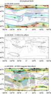 |
Fig. 4. Sixty-one-day mean daily amplitude of the northward magnetic perturbations for the control case (MC2008; panel a) and the difference with C1908 and M1908 (panels b/c). Contours for the difference plots are at 0, ±5, ±10, ±20, and ±50 nT. Light (dark) shading indicates statistical significance at the 95% (99%) level. |
In contrast, changes in the main magnetic field have widespread effects on the daily amplitude of the magnetic perturbations (panel c). At low- to mid-latitudes, where the Sq current system is located, changes on the order of ±5 nT are quite common, but close to the magnetic equator they can be larger still: up to ±10 nT for the eastward and downward components (not shown) or even ±20 nT for the northward component. These changes correspond to about 50% of the total amplitude, and are highly significant. The pattern of change is due to both changes in the geographic location of the magnetic equator and changes in magnetic field strength (Cnossen & Richmond 2013).
Some significant changes are also found at higher latitudes, but this result may be less reliable, as magnetic perturbations at high latitudes are more sensitive to magnetospheric processes, which are not represented in the TIE-GCM used here. Still, it illustrates the possibility that magnetic perturbations at high latitudes could also be affected by main magnetic field changes, which should be investigated further with a more appropriate model. If long-term changes in the geomagnetic field affect the magnetic perturbations associated with geomagnetic storms, this could have important implications for the interpretation of reported trends in geomagnetic activity (e.g., Stamper et al. 1999; Clilverd et al. 2002).
4. Discussion and conclusions
We have presented a quantitative comparison between the effects of enhanced CO2 levels and the changing geomagnetic field on the upper atmosphere, based on simulations with the TIE-GCM. Our simulations show very clearly how little influence the increase in CO2 concentration has had on foF2 and the daily magnetic perturbations associated with the Sq current system compared to changes in the Earth’s magnetic field. Both factors contribute to long-term changes in hmF2, but the increase in CO2 level produces a rather uniform decrease in hmF2 of about 5 km, while magnetic field changes produce changes in hmF2 of similar order of magnitude as well as much larger changes, depending on location (up to +40 and −60 km in the Atlantic region). Magnetic field changes are thus much more likely to be responsible for observed long-term trends in foF2 and Sq amplitude than the increase in CO2 concentration, and they are at least as important as, but can be considerably more important than, the increase in CO2 concentration for long-term trends in hmF2.
Ion temperature is affected in roughly equal measures (~10 K) by magnetic field changes and increased CO2 levels, when only significant effects are considered. Magnetic field changes cause either cooling or warming, depending on location, while the increase in CO2 concentration results in cooling everywhere. Changes in the magnetic field cause nearly no significant change in neutral temperature. Still, they do substantially alter the pattern of change predicted for the increase in CO2 concentration alone and its statistical significance. In particular over northern America and parts of the Pacific and Atlantic Oceans, the decrease in temperature simulated for changes in the magnetic field and CO2 concentration combined is up to twice as large as simulated for the CO2 increase alone, and also its significance is broadened in those regions. Both processes are therefore important. Also more generally, we may conclude that to understand climatic changes in the upper atmosphere, it is necessary to consider combinations of effects from different drivers of long-term change rather than to focus on only one potential driver.
Our simulations also show that long-term changes in neutral temperature (and therefore neutral density), do not necessarily need to be consistent with long-term trends in ionospheric variables, such as hmF2, foF2, or ion temperature, as they may in part arise from different processes. For instance, comparing Figures 1 and 2, we find that changes in neutral temperature and changes in ion temperature share some characteristics, but they are not identical; differences are mainly due to differences in the responses of ion and neutral temperatures to the effects of magnetic field changes. This offers a possible explanation for the inconsistency noted by Akmaev (2012) between reported long-term trends in ion temperature and observed trends in global mean neutral density in the thermosphere.
Long-term trends in the upper atmosphere do also not need to be spatially homogeneous. Unlike the effects of increased CO2 levels, the effects of the changing geomagnetic field are distinctly non-uniform across the globe, which could help explain why different long-term trends, sometimes even of the opposite sign, have been observed at different ionosonde stations. This result implies as well that the study of spatial patterns of long-term trends could reveal important clues to the causes of those trends.
Of course, the results presented here rely solely on simulations with the TIE-GCM. While the TIE-GCM is one of the best models in its category, it is not a perfect representation of the true upper atmosphere and there are uncertainties associated with any model simulation. For instance, there are limited constraints available on the CO2-O relaxation rate coefficient, which determines in part how efficiently CO2 cools the upper atmosphere (Sharma & Roble 2002). This means that a reasonable choice has to be made, and this choice will have an influence on the effect the model predicts for an increase in the CO2 concentration. Still, results on the effects of CO2 increases obtained with the TIE-GCM are in quite good agreement with results obtained with other models (e.g. Cnossen 2012), which gives some confidence that the results are likely to be fairly realistic. Effects of changes in the magnetic field have so far mainly been investigated with the TIE-GCM and the related CMIT model. Only one other modeling study by Yue et al. (2008) confirms the importance of geomagnetic field changes for long-term trends in hmF2 and foF2 at low- to mid-latitudes, but they did not investigate effects on ion or neutral temperature. Independent studies with other numerical models of the thermosphere-ionosphere system to verify the effects of changes in the geomagnetic field would therefore be particularly welcome.
Quantitative comparisons with observed trends are needed to find out to what extent the combined effects of the increase in CO2 concentration and magnetic field changes can explain these trends. Recent comparisons of observed trends with the simulations carried out by Cnossen & Richmond (2013) indicate that magnetic field changes could be responsible for most of the trends in Sq amplitude at three out of five of the stations that were investigated (De Haro Barbas et al. 2013), while they could only explain about 8% of the observed trend in ion temperature at Millstone Hill (Zhang & Holt 2013). It still remains unclear whether the increase in CO2 concentration could be responsible for the remainder, although this seems unlikely based on the results shown here. Perhaps other processes should be considered as well, such as long-term solar variability or climatic changes in the atmosphere below, which could affect the upper atmosphere, for instance, through changes in gravity wave generation and/or propagation conditions (e.g. Oliver et al. 2013). To facilitate further comparisons between model predictions and observed trends we will make the output from the simulations presented here, including results for different vertical levels, local/universal times, or different variables, where available, freely available to the community on request (contact the author if interested).
Acknowledgments
This study is part of the British Antarctic Survey Polar Science for Planet Earth Programme. It was funded by Natural Environment Research Council (NERC) fellowship NE/J018058/1. The TIE-GCM simulations used in this study were performed on the Yellowstone high-performance computing facility (ark:/85065/d7wd3xhc) provided by NCAR’s Computational and Information Systems Laboratory, sponsored by the National Science Foundation.
References
- Akmaev, R.A., On estimation and attribution of long-term temperature trends in the thermosphere, J. Geophys. Res., 117, A09321, 2012. [Google Scholar]
- Akmaev, R.A., V.I. Fomichev, and X. Zhu, Impact of middle-atmospheric composition changes on greenhouse cooling in the upper atmosphere, J. Atmos. Sol. Terr. Phys., 68 (17), 1879–1889, 2006. [CrossRef] [Google Scholar]
- Bremer, J., Ionospheric trends in mid-latitudes as a possible indicator of the atmospheric greenhouse effect, J. Atmos. Terr. Phys., 54 (11–12), 1505–1511, 1992. [CrossRef] [Google Scholar]
- Bremer, J., Trends in the ionospheric E and F regions over Europe, Ann. Geophys., 16, 986–996, 1998. [Google Scholar]
- Bremer, J., Long-term trends in the ionospheric E and F1 regions, Ann. Geophys., 26, 1189–1197, 2008. [Google Scholar]
- Bremer, J., T. Damboldt, J. Mielich, and P. Suessmann, Comparing long-term trends in the ionospheric F2-region with two different methods, J. Atmos. Sol. Terr. Phys., 77, 174–185, 2012. [CrossRef] [Google Scholar]
- Clilverd, M.A., T.D.G. Clark, E. Clarke, H. Rishbeth, and T. Ulich, The causes of long-term changes in the aa index, J. Geophys. Res., 107 (A12), 14–41, 2002. [Google Scholar]
- Cnossen, I., Climate change in the upper atmosphere. In: G., Liu, Editor. Greenhouse gases-emission, measurement and management, InTech, pp. 315–336, 2012. [Google Scholar]
- Cnossen, I., and A.D. Richmond, Modelling the effects of changes in the Earth’s magnetic field from 1957 to 1997 on the ionospheric hmF2 and foF2 parameters, J. Atmos. Sol. Terr. Phys., 70, 1512–1524, 2008. [CrossRef] [Google Scholar]
- Cnossen, I., and A.D. Richmond, How changes in the tilt angle of the geomagnetic dipole affect the coupled magnetosphere-ionosphere-thermosphere system, J. Geophys. Res., 117, A10317, DOI: 10.1029/2012JA018056, 2012. [CrossRef] [Google Scholar]
- Cnossen, I., and A.D. Richmond, Changes in the Earth’s magnetic field over the past century: Effects on the ionosphere-thermosphere system and solar quiet (Sq) magnetic variation, J. Geophys. Res., 118, 849–858, DOI: 10.1029/2012JA018447, 2013. [CrossRef] [Google Scholar]
- Cnossen, I., A.D. Richmond, M. Wiltberger, W. Wang, and P. Schmitt, The response of the coupled magnetosphere-ionosphere-thermosphere system to a 25% reduction in the dipole moment of the Earth’s magnetic field, J. Geophys. Res., 116, A12304, DOI: 10.1029/2011JA017063, 2011. [CrossRef] [Google Scholar]
- Cnossen, I., A.D. Richmond, and M. Wiltberger, The dependence of the coupled magnetosphere-ionosphere-thermosphere system on the Earth’s magnetic dipole moment, J. Geophys. Res., 117, A05302, DOI: 10.1029/2012JA017555, 2012. [Google Scholar]
- De Haro Barbas, B.F., A.G. Elias, I. Cnossen, and M. Zossi de Artigas, Long-term changes in solar quiet (Sq) geomagnetic variations related to Earth’s magnetic field secular variation, J. Geophys. Res., 118, 3712–3718, DOI: 10.1002/jgra.50352, 2013. [CrossRef] [Google Scholar]
- Donaldson, J.K., T.J. Wellman, and W.L. Oliver, Long-term change in thermospheric temperature above Saint Santin, J. Geophys. Res., 115, A11305, 2010. [Google Scholar]
- Doumbia, V., A. Maute, and A.D. Richmond, Simulation of equatorial electrojet magnetic effects with the thermosphere-ionosphere-electrodynamics general circulation model, J. Geophys. Res., 112, A09309, 2007. [Google Scholar]
- Elias, A.G., and N. Ortiz de Adler, Earth magnetic field and geomagnetic activity effects on long-term trends in the F2 layer at mid-high latitudes, J. Atmos. Sol. Terr. Phys., 68, 1871–1878, 2006. [CrossRef] [Google Scholar]
- Elias, A.G., M. Zossi de Artigas, and B.F. de Haro Barbas, Trends in the solar quiet geomagnetic field variation linked to the Earth’s magnetic field secular variation and increasing concentrations of greenhouse gases, J. Geophys. Res., 115, A08316, 2010. [Google Scholar]
- Emmert, J.T., J.M. Picone, J.L. Lean, and S.H. Knowles, Global change in the thermosphere: Compelling evidence of a secular decrease in density, J. Geophys. Res., 109, A02301, 2004. [Google Scholar]
- Emmert, J.T., and J.M. Picone, Statistical uncertainty of 1967–2005 thermospheric density trends derived from orbital drag, J. Geophys. Res., 116, A00H09, 2011. [Google Scholar]
- Finlay, C.C., S. Maus, C.D. Beggan, et al., International Geomagnetic Reference Field: the eleventh generation, Geophys. J. Int., 183, 1216–1230, 2010. [Google Scholar]
- Hagan, M.E., and J.M. Forbes, Migrating and nonmigrating diurnal tides in the middle and upper atmosphere excited by tropospheric latent heat release, J. Geophys. Res., 107 (D24), 4754, DOI: 10.1029/2001JD001236, 2002. [CrossRef] [Google Scholar]
- Hagan, M.E., and J.M. Forbes, Migrating and nonmigrating semidiurnal tides in the upper atmosphere excited by tropospheric latent heat release, J. Geophys. Res., 108, 1062, DOI: 10.1029/2002JA009466, 2003. [CrossRef] [Google Scholar]
- Heelis, R.A., J.K. Lowell, and R.W. Spiro, A model of the high-latitude ionospheric convection pattern, J. Geophys. Res., 87, 6339–6345, 1982. [Google Scholar]
- Jarvis, M.J., B. Jenkins, and G.A. Rodgers, Southern hemisphere observations of a long-term decrease in F region altitude and thermospheric wind providing possible evidence for global thermospheric cooling, J. Geophys. Res., 103, 20774–20787, 1998. [Google Scholar]
- Keating, G.M., R.H. Tolson, and M.S. Bradford, Evidence of long term global decline in the Earth’s thermospheric densities apparently related to anthropogenic effects, Geophys. Res. Lett., 27, 1523–1526, 2000. [CrossRef] [Google Scholar]
- Laštovička, J., S.C. Solomon, and L. Qian, Trends in the neutral and ionized upper atmosphere, Space Sci. Rev., 168, 113–145, 2012. [Google Scholar]
- Maeda, S., T.J. Fuller-Rowell, and D.S. Evans, Heat budget of the thermosphere and temperature variations during the recovery phase of a geomagnetic storm, J. Geophys. Res., 97, 14947–14957, 1992. [CrossRef] [Google Scholar]
- Oliver, W.L., S.-R. Zhang, and L.P. Goncharenko, Is thermospheric global cooling caused by gravity waves? J. Geophys. Res., 118, 3898–3908, 2013. [CrossRef] [Google Scholar]
- Qian, L., A.G. Burns, S.C. Solomon, and R.G. Roble, The effect of carbon dioxide cooling on trends in the F2-layer ionosphere, J. Atmos. Sol. Terr. Phys., 71, 1592–1601, 2009. [Google Scholar]
- Qian, L., A.G. Burns, B.A. Emery, B. Foster, G. Lu, A. Maute, A.D. Richmond, R.G. Roble, S.C. Solomon, and W. Wang, The NCAR TIE-GCM: A community model of the coupled thermosphere/ionosphere system. In: J.D., Huba, R.W. Schunk, and G. Khazanov, Editors. Modeling the Ionosphere-Thermosphere System, vol. 201, p. 73–83, Am. Geophys. Union monograph, ISBN 978-0-87590-491-7, DOI: 10.1002/9781118704417.ch7, 2014. [Google Scholar]
- Richmond, A.D., E.C. Ridley, and R.G. Roble, A thermosphere/ionosphere general circulation model with coupled electrodynamics, Geophys. Res. Lett., 19 (6), 601–604, 1992. [Google Scholar]
- Richmond, A.D., and A. Maute, Ionospheric electrodynamics modeling. In: J.D., Huba, R.W. Schunk, and G. Khazanov, Editors. Modeling the Ionosphere-Thermosphere System, Am. Geophys. Union monograph, vol. 201, p. 57–71, ISBN 978-0-87590-491-7, DOI: 10.1002/9781118704417.ch6, 2014. [CrossRef] [Google Scholar]
- Rishbeth, H., A greenhouse effect in the ionosphere, Planet. Space Sci., 38 (7), 945–948, 1990. [Google Scholar]
- Rishbeth, H., and R.G. Roble, Cooling of the upper atmosphere by enhanced greenhouse gases–modelling of thermospheric and ionospheric effects, Planet. Space Sci., 40 (7), 1011–1026, 1992. [Google Scholar]
- Roble, R.G., and R.E. Dickinson, How will changes in carbon dioxide and methane modify the mean structure of the mesosphere and thermosphere, Geophys. Res. Lett., 16 (12), 1441–1444, 1989. [Google Scholar]
- Roble, R.G., E.C. Ridley, A.D. Richmond, and R.E. Dickinson, A coupled thermosphere/ionosphere general circulation model, Geophys. Res. Lett., 15 (12), 1325–1328, 1988. [Google Scholar]
- Sharma, R.D., and R.G. Roble, Cooling mechanisms of the planetary thermospheres: they key role of O atom vibrational excitation of CO2 and NO, Chem. Phys. Chem., 3, 841–843, 2002. [CrossRef] [Google Scholar]
- Stamper, R., M. Lockwood, M.N. Wild, and T.D.G. Clark, Solar causes of the long-term increase in geomagnetic activity, J. Geophys. Res., 104 (A12), 28325–28342, 1999. [CrossRef] [Google Scholar]
- Torta, J.M., L.R. Gaya-Piqué, J.J. Curto, and D. Altadill, An inspection of the long-term behaviour of the range of the daily geomagnetic field variation from comprehensive modelling, J. Atmos. Sol. Terr. Phys., 71, 1497–1510, 2009. [CrossRef] [Google Scholar]
- Ulich, T., and E. Turunen, Evidence for long-term cooling of the upper atmosphere in ionosonde data, Geophys. Res. Lett., 24, 1103–1106, 1997. [Google Scholar]
- Upadhyay, H.O., and K.K. Mahajan, Atmospheric greenhouse effect and ionospheric trends, Geophys. Res. Lett., 25, 3375–3378, 1998. [CrossRef] [Google Scholar]
- Yue, X., L. Liu, W. Wan, Y. Wei, Z. Ren, Modeling the effects of secular variation of geomagnetic field orientation on the ionospheric long term trend over the past century, J. Geophys. Res., 113, A10301, 2008. [CrossRef] [Google Scholar]
- Zhang, S.-R., J.M. Holt, Long-term ionospheric cooling: dependency on local time, season, solar activity and geomagnetic activity, J. Geophys. Res., 118, 3719–3730, DOI: 10.1002/jgra.50306, 2013. [Google Scholar]
- Zhang, S.-R., J.M. Holt, J. Kurdzo, Millstone Hill ISR observations of upper atmospheric long-term changes: Height dependency, J. Geophys. Res., 116, A00H05, 2011. [Google Scholar]
Cite this article as: Cnossen I.: The importance of geomagnetic field changes versus rising CO2 levels for long-term change in the upper atmosphere. J. Space Weather Space Clim., 2014, 4, A18.
All Tables
All Figures
|
Fig. 1. Sixty-one-day mean neutral temperature for the control case (MC2008; panel a) and the difference with C1908, M1908, and MC1908 (panels b–d) at 12 LT at a pressure level of 3.2 × 10⁻⁸ hPa (~300 km). The contour interval for the difference plots is 2 K between −12 and +12 K, with an additional contour at −16 K for the bottom panel. Light (dark) shading indicates statistical significance at the 95% (99%) level. |
| In the text | |
|
Fig. 2. Sixty-one-day mean ion temperature for the control case (MC2008; panel a) and the difference with C1908, M1908, and MC1908 (panels b–d) at 12 LT at a pressure level of 3.2 × 10⁻⁸ hPa (~300 km). Contours for the difference plots are at 0, ±10, ±25, ±50, and ±100 K. Light (dark) shading indicates statistical significance at the 95% (99%) level. |
| In the text | |
|
Fig. 3. Sixty-one-day mean hmF2 (left) and foF2 (right) for the control case (MC2008; panels a/e) and the difference with C1908, M1908, and MC1908 (panels b/f, c/g, and d/h, respectively) at 12 LT. The contour interval for the hmF2 difference plots is 20 km between −60 and +60 km, with additional contours at −5 and +5 km. The contour interval for the foF2 difference plots is 0.25 MHz between −1.5 and +1.5 MHz. Light (dark) shading indicates statistical significance at the 95% (99%) level. |
| In the text | |
|
Fig. 4. Sixty-one-day mean daily amplitude of the northward magnetic perturbations for the control case (MC2008; panel a) and the difference with C1908 and M1908 (panels b/c). Contours for the difference plots are at 0, ±5, ±10, ±20, and ±50 nT. Light (dark) shading indicates statistical significance at the 95% (99%) level. |
| In the text | |
Current usage metrics show cumulative count of Article Views (full-text article views including HTML views, PDF and ePub downloads, according to the available data) and Abstracts Views on Vision4Press platform.
Data correspond to usage on the plateform after 2015. The current usage metrics is available 48-96 hours after online publication and is updated daily on week days.
Initial download of the metrics may take a while.