© J. Feltens et al., Published by EDP Sciences 2018

1 Introduction

Atmospheric delays are significant contributors to the error budget of satellite tracking. The total atmospheric effect on satellite signals comprises two major parts: 1) the contribution from the troposphere and 2) the contribution from the ionosphere (e.g. Seeber, 2003). The troposphere is the neutral lower part of the Earth atmosphere extending from ground up to 50 km (stratosphere included). For frequencies below 30 GHz, the troposphere is a non-dispersive medium, i.e. the tropospheric range delays do not depend on satellite signal frequency. For mathematical modelling, the troposphere can be described as a mixture of two ideal gases: dry air and water vapour, whereby the dry part contributes about 90% of the total tropospheric refraction and the wet part the remaining 10%. Typical total tropospheric range delays are between 2.3 m in zenith direction and up to almost 30 m at low elevations (e.g. Seeber, 2003). Above the troposphere resides the ionosphere, extending from 50 km up to about 2000 km, where it transits into the plasmasphere, which smoothly transfers into the interplanetary plasma at several 10000 km altitude (e.g. Davies, 1990). There exist no sharp transitions between ionosphere, plasmasphere and interplanetary plasma. Ratcliffe (1972) uses the following formulation to describe nicely the ionosphere as “The part of the atmosphere above about 60 km, where free electrons exist in numbers sufficient to influence the travel of radio waves …”. The ionization in the ionosphere is primarily triggered by solar radiation. In addition, the composition of atmospheric gases at different altitudes, the geomagnetic field, transport and recombination processes play an important role to establish the typical ionospheric structures in terms of different layers, equatorial anomaly, auroral oval, etc.; the interested reader is referred at this point to the pertinent literature (e.g. Davies, 1990; Ratcliffe, 1972; Komjathy, 1997; Kelley, 1989). In contrast to the troposphere, the ionosphere is a dispersive medium, i.e. the delay a radio signal suffers by the ionosphere depends on the signal's frequency. Typical values of ionospheric range delays (for single-frequency measurements) range between 10 cm and up to 500 m. Ionospheric range delays are inversely proportional to the square of the satellite carrier frequency and depend on elevation (e.g. Seeber, 2003).

ESOC Flight Dynamics has to apply tropospheric and ionospheric corrections to the tracking data of ESA spacecraft (range, Doppler, delta-DOR) to achieve accurate orbit determinations (OD), especially for the interplanetary space probes. In addition for delta-DOR (http://www.esa.int/Our_Activities/Operations/About_delta_DOR), these media calibrations are also needed for quasar tracking. Concerning frequency bands used, there is currently a change ongoing from S-Band tracking to X-Band and Ka-Band tracking; S-Band is actually no longer used at ESA for tracking deep-space missions. Thus the troposphere is considered to be the dominant term while the ionosphere becomes less significant.

So far, ESOC Flight Dynamics has computed its tropospheric and ionospheric calibrations in-house based on empirical background models (Saastamoinen, 1973, Klobuchar, 1975, Jakowski et al., 2011) or, under specific agreements, received support from the Jet Propulsion Laboratory (JPL) in Pasadena, California, U.S.A, in the form of time-normalized polynomials. These polynomials will be described in detail in Section 3. On the other hand, the ESOC Navigation Support Office generates as part of its routine Global Navigation Satellite Systems (GNSS) data processing for the International GNSS Service (IGS, http://www.igs.org/) GNSS orbit and clocks data, tropospheric zenith delays and ionospheric slant Total Electron Content (sTEC) observables, among others, on regular basis (http://navigation-office.esa.int/about/activities/). In addition, the ESOC Navigation Support Office operates and maintains its ESA's GNSS Observation Network (EGON) permanently recording multi-frequency data (http://navigation-office.esa.int/ESA's_GNSS_Observation_Network_(EGON).html), and some of these stations are also equipped with WEather STation (WEST) meteorological data recorders. These WEST data instruments belong to the ESOC Ground Systems Engineering Department. − So an in-house generation of media calibrations by using this data is an obvious task, with the target to be as independent as possible from external data and models.

The ground stations to be supported are primarily the three ESA Deep Space Network (DSN) sites Cebreros/Spain (CEBR), Malargüe/Argentina (MGUE) and New Norcia/Australia (NNOR) (http://www.esa.int/Our_Activities/Operations/Estrack). Further sites may be included in future.

The rest of this paper is structured as follows: Section 2 points out general aspects of the algorithms design and concepts. Section 3 explains how the tropospheric calibrations are computed. Section 4 explains how the ionospheric calibrations are computed. Section 5 presents results obtained with the newly established media calibration service provided by the Navigation Support Office to Flight Dynamics. Section 6 concludes the paper by summarizing the new media calibrations service implementation at ESOC. Finally Appendix A provides some supplementing algorithms for ionospheric intersection point (IPP) position vector computation, which is needed for the ionospheric media calibrations computation.

2 Principles for new approach to compute media calibrations

Three key points were important when working out the concept for this new in-house media calibrations service:

• independency from external (especially non-ESA) sources in terms of data, models and software as far as possible. − Nevertheless, global GNSS data collected with the IGS network is needed to get high-precision orbits and clocks, which are required to obtain reliable tropospheric zenith delay solutions, Section 3;

• well suited for operational needs: Algorithms are simple and robust, optimized for efficient coding;

• consideration of alternatives to retain the service in cases when ESA observation data (GNSS, meteo data from the ground sites) recording is interrupted.

With regard to the above three key points, the algorithms to compute the tropospheric calibrations, Section 3, and the ionospheric calibrations, Section 4, were designed in a way that they rely on ESA observation data as far as possible and on models as less as possible. It is assumed that an empirical approach based on observation data better reflects, apart from measurement errors and noise, the actual status of the troposphere/ionosphere rather than a model typically describing some mean or smoothed troposphere/ionosphere. Therefore the usage of models is foreseen in the algorithms presented in Sections 3 and 4 only in cases of non-availability of observation data.

3 Tropospheric media calibrations

3.1 Tropospheric calibrations provided by JPL

Historically, tropospheric media calibrations processing at ESOC Flight Dynamics is aligned to JPL data formats, which may change in future. So the essentials of tropospheric calibrations provided by JPL (JPL, 2008) are summarized in the following for a better understanding of the own new approach, Section 3.2:

• assumption of azimuthal symmetry, i.e. no gradients;

• neither spacecraft- nor frequency-specific;

• tropospheric calibrations are represented per station and in 6^h time intervals by one time-normalized polynomial for the wet (ZWD) − and one time-normalized polynomial for the dry zenith delay (ZHD), Eq. (2);

• JPL employs the Niell Mapping Function (NMF) (Niell, 1996, 2000) to compute slant range tropospheric corrections of these ZWDs and ZHDs. − The NMF is a function of season, station latitude and height, but not of surface meteorological data;

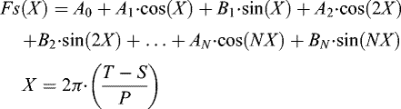
• the 1^st order (or background) tropospheric calibration is computed with so-called seasonal models for the ZWD and ZHD component (JPL, 2008; Chao, 1973) which do not depend on real-time data. The seasonal model parameters are delivered to the user in form of a time-normalized Fourier series representation, separately for the ZWD and ZHD:

$$\begin{array}{c}\hfill Fs\left(X\right)=A_0+A_1\cdot \cos \left(X\right)+B_1\cdot \sin \left(X\right)+A_2\cdot \cos \left(2X\right)+B_2\cdot \sin \left(2X\right)+\dots +A_N\cdot \cos \left(NX\right)+B_N\cdot \sin \left(NX\right)\hfill \\ \hfill \mathrm{}\hfill \\ \hfill X=2\pi \cdot \left(\frac{T-S}{P}\right)\hfill \end{array}$$(1)

A_i, B_i – fitted Fourier coefficients;

N – degree of Fourier series expansion;

T – calibration time [sec];

S – start time [sec];

P – period of fundamental mode [sec].

The seasonal models, as well as the JPL media calibrations in general, are delivered to the users in the Control Statement Processor (CSP) format (JPL, 2008);

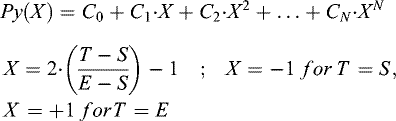
• on top of these ZWD and ZHD background calibrations, time series of delta-corrections of tropospheric zenith delays, wet and dry, are derived from near-real-time weather and GPS data and delivered to the users in form of normalized-time polynomial representations:

$$\begin{array}{c}\hfill Py\left(X\right)=C_0+C_1\cdot X+C_2\cdot X^2+\dots +C_N\cdot X^N\hfill \\ \hfill \mathrm{}\hfill \\ \hfill \begin{array}{ccc}\hfill X=2\cdot \left(\frac{T-S}{E-S}\right)-1\hfill & \hfill ;\hfill & \hfill X=-1_{\mathrm{}}for{}_{\mathrm{}}T=S_{\mathrm{}},{}_{\mathrm{}}X=+1_{\mathrm{}}for{}_{\mathrm{}}T=E\hfill \end{array}\hfill \end{array}$$(2)

C_i – fitted polynomial coefficients;

N – degree of polynomial representation;

T – calibration time [sec];

S – start time [sec];

E – end time [sec].

The Eq. (2) polynomial representation is used to compute both the wet and dry delta-corrections. The user has then to calculate the actual tropospheric zenith delay, separately for wet and dry, as sum of the value obtained from the seasonal model (background) plus the delta-correction computed with the actual polynomial.

3.2 Computation of tropospheric calibrations by the ESOC Navigation Support Office

Tropospheric media calibrations are independent of spacecraft and, below 30 GHz, also of frequency. Thus per day, one ACSII file is produced in CSP-format by the ESOC Navigation Support Office, listing for ESA's three DSN sites CEBR, MGUE, NNOR polynomial representations of wet and dry delta-zenith delays in 6 hour time intervals. Such a CSP-file is generated once per day for the day before in rapid mode. In final mode the same process is repeated with 4 days latency and more GNSS observation data. Each polynomial representation, Eq. (2), describes then wet and dry delta-zenith delays w.r.t. the background ZWD and ZHDs computed with the seasonal model.

Before entering into the polynomial fit, Eqs. (3)–(5), the tropospheric zenith delay values are preprocessed as follows:

• a SINEX.tro file (ftp://igs.org/pub/data/format/sinex_tropo.txt) obtained from daily routine GNSS processing at the Navigation Support Office provides 48^h time series of total tropospheric zenith delays (ZTDs) and ZWDs for all stations considered (Fig. 1);

• in addition, at the ESA DSN sites CEBR, MGUE, NNOR, WEather STation (WEST) data is permanently recorded and enters into the media calibrations process as 1 minute samples. The WEST data comprise, among others, temperature, pressure and humidity;

• detection and removal of large outliers from the tropospheric zenith delay series;

• the Saastamoinen (1973) Model is employed to compute the ZHD component of the ZTD with the WEST data. In the case that pressure data from the WEST stations is not available, corresponding weather parameters are computed with the Global Pressure and Temperature model (GPT) (Böhm, 2007; Steigenberger et al., 2009; Lagler et al., 2013);

• the ZHDs are corrected for the height difference between the GNSS/IGS antenna on DSN site, w.r.t. which the GNSS measurements and parameter estimation were made, and the reference point of the DSN antenna (point of antenna azimuth axis with elevation axis crossing), using a formula of Estefan and Sovers (1994);

• the ZTDs and ZWDs provided in the SINEX.tro file were determined by using temperature and pressure values from the GPT model; this is basically a setup for the routine IGS processing. On the other hand, Flight Dynamics prefers, due to its systems setup, to get its tropospheric calibrations referred to the Saastamoinen Model, with the dry part computed from WEST data pressure measurements. Thus the ZHDs computed with the Saastamoinen Model from WEST data, are subtracted from the ZTDs of the SINEX.tro file, leading to ZWDs referred to the Saastamoinen Model. − The ZWDs provided directly by the SINEX.tro file are in this way ignored for tropospheric media calibrations processing;

• the JPL wet and dry seasonal model is subtracted from the above ZWD and ZHD series, resulting in corresponding delta-ZWD and delta-ZHD (δZWD and δZHD) time series into which polynomial expressions, Eq. (2), are then fitted, Eqs. (3)–(5).

For the tropospheric media calibrations service, the Navigation Support Office produces once per day a SINEX.tro file containing 48^h time series of ZWDs and ZTDs for all DSN sites considered. Processing is done in rapid and in final mode. In rapid mode, this computer run is submitted via an automatic job scheduler (crontab) every day at 14:30 UT and covers the time interval from 12:00 UT of today (observation day) 48^h backwards to 12:00 UT of the day before yesterday. In a subsequent computer run, this SINEX.tro file enters as input into the polynomials fitting and CSP-file generation. In final mode, the same process is repeated at 02:02 UT, 4 days after the end of the observation day, with more observation data.

Figure 1 shows how these computer runs of 48^h SINEX data generation are scheduled for a sequence of several days i, i + 1, i + 2, i + 3, … Also indicated are the rapid mode launch times at 14:30 UT. The 48^h run of each day is processed independently of the other days. Of this 48^h series of ZWDs and ZTDs, δZWD and δZHD series are then established as described above. Into the δZWD and δZHD series thus obtained, separately for wet and dry, a sequence of eight 6^h polynomial representations is fitted. In order to avoid jumps at the interfaces between one polynomial representation and the next, the eight 6^h polynomials sequence is fitted to the complete 48^h delta-zenith delays series within one fitting process, as indicated in Eq. (5). In order to suppress jumps at the interfaces, constraints are introduced between successive polynomial representations in terms of offset, slope and slope rate, depending on the user's setting. Constraints are introduced between two successive polynomial representations in terms of conditional Eqs. (3.3a–c): $$\mathrm{O}\mathrm{f}\mathrm{f}\mathrm{s}\mathrm{e}\mathrm{t}:\begin{array}{ccc}\hfill P\left({\mathrm{X}}_E\right)=Q\left({\mathrm{Y}}_S\right)\hfill & \hfill \to \hfill & \hfill 0=Q\left({\mathrm{Y}}_S\right)-P\left({\mathrm{X}}_E\right)\hfill \end{array}$$(3a) $$\mathrm{S}\mathrm{l}\mathrm{o}\mathrm{p}\mathrm{e}:\begin{array}{ccc}\hfill P^{\prime }\left({\mathrm{X}}_E\right)=Q^{\prime }\left({\mathrm{Y}}_S\right)\hfill & \hfill \to \hfill & \hfill 0=Q^{\prime }\left({\mathrm{Y}}_S\right)-P^{\prime }\left({\mathrm{X}}_E\right)\hfill \end{array}$$(3b) $$\mathrm{S}\mathrm{l}\mathrm{o}\mathrm{p}\mathrm{e}\mathrm{r}\mathrm{a}\mathrm{t}\mathrm{e}:\begin{array}{ccc}\hfill P^{\prime }\left({\mathrm{X}}_E\right)=Q^{\prime }\left({\mathrm{Y}}_S\right)\hfill & \hfill \to \hfill & \hfill 0=Q^{\prime }\left({\mathrm{Y}}_S\right)-P^{\prime }\left({\mathrm{X}}_E\right)\hfill \end{array}$$(3c) where$P\left({\mathrm{X}}_E\right),P^{\prime }\left({\mathrm{X}}_E\right),P^{\prime }\left({\mathrm{X}}_E\right)$ – 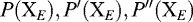function, 1^st and 2^nd derivative of preceding polynomial;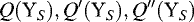$Q\left({\mathrm{Y}}_S\right),Q^{\prime }\left({\mathrm{Y}}_S\right),Q^{\prime }\left({\mathrm{Y}}_S\right)$ – function, 1^st and 2^nd derivative of subsequent polynomial.

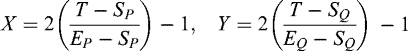
The polynomial arguments are computed according to Eq. (2): $$\begin{array}{cc}\mathit{X}=2\left(\frac{T-S_P}{E_P-S_P}\right)-1,& \mathit{Y}=2\left(\frac{T-S_Q}{E_Q-S_Q}\right)\end{array}-1$$(4) where

X – argument of preceding polynomial;

Υ – argument of subsequent polynomial;

S_P, E_P – start/end time of preceding polynomial;

S_Q, E_Q – start/end time of subsequent polynomial.

The interface epoch between the two successive polynomial representations is defined by the end time E_P of the preceding polynomial P(X), which is equal to the start time S_Q of the subsequent polynomial Q(Y), i.e. E_P = S_Q. Putting these values for T into Eq. (4) leads to X_E = +1 and Y_S = −1 as arguments for the constraining Eq. (3a–c):

There is an agreement with Flight Dynamics that the polynomial representation for the tropospheric media calibrations should be of polynomial degree Four. This choice was a consequence of a trial and error process, during which it was observed that in some cases high degree polynomials were following the noise of the zenith delay estimates, which are uncorrelated and not smoothed, thus creating artificial slopes in the calibrations that were worsening the results.

Equation (5) displays the observation equations structure of two successive polynomial representations P(X) and Q(Y) with the interface constraints between them. These constraining equations are multiplied with weights W_offs, W_slpe, W_slrt, which can be set by the user. Optimal values for these weights were found out by trying: W_offs = 100, W_slpe = 100, W_slrt = 0. An introduction of a Zero-weight leads to a non-constraining of the respective parameter, i.e. the slope rate is with the actual setting not constrained. But principally the slope rate could be constrained too and is thus marked with “eventually” in Eq. (5).

In the ideal case, the interface epochs of the eight polynomial representations coincide with measurement epochs of the tropospheric zenith delays. In this way, the last delta-tropospheric zenith delay (δTZD, standing here for δZWD or δZHD) value of the preceding polynomial is also the first delta-zenith delay value of the subsequent polynomial, i.e. this delta-zenith delay value appears twice in the observation equations (δTZD_m in Eq. (5)). For the sake of simplicity and better readability, Eq. (5) is set up here for 3^rd degree polynomial representations only and only for a sequence of two successive polynomial representations. 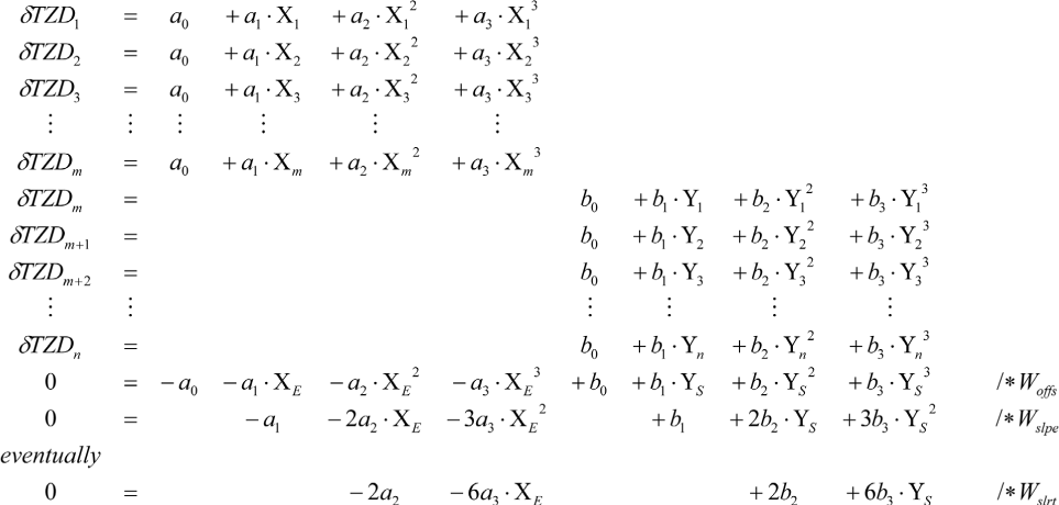$$\mathrm{See\; Formula\; in\; PDF}$$(5) Figure 2 displays the principal structure of the complete A-matrix for a 8 × 6^h polynomials fit, also for the ideal case of no gaps in the tropospheric zenith delay data and tropospheric zenith delay epochs coinciding with the interface epochs of the polynomial representation time spans. For simplicity, only three tropospheric zenith delay epochs are shown for each polynomial representation.

So, in summary, one A-matrix is set up and solved in a least squares fit to obtain the estimated coefficients for all polynomials.

Equation (5) and Figure 2 represent the ideal case in terms of full tropospheric zenith delay data availability and tropospheric zenith delay epochs coinciding with the interface epochs of the eight polynomial representations. However, deviations in tropospheric zenith delay values availability and distribution from these ideal conditions can happen in daily routine operational processing. Thus the above described approach had to be enabled to handle also such cases:

• in the case that an interface epoch does not coincide with one of the tropospheric zenith delay epochs, the fit of the preceding polynomial takes all δTZD values falling with their epochs into its respective representation time interval and the fit of the subsequent polynomial takes all δTZD values falling with their epochs into its respective representation time interval, i.e. no δTZD value will, due to non-existence, be introduced twice at the interface epoch. The constraining equations will, nevertheless, be established at the interface epoch;

• if in a given polynomial representation time span the number of available δTZD values is due to gaps less or equal to the specified polynomial degree, the polynomial degree is for that time span set to One (linear fit) in the case that at least two δTZD observables are available and that the affected 6^h interval is not the first or the last interval of the 8 × 6^h polynomials fit. If only one observable is available and/or the affected interval is not the first or the last interval of the 8 × 6^h polynomials fit, the polynomial degree is set to Zero (constant fit). This processing scheme is retained as long as at least one observable falls into the respective time interval. This approach of setting the polynomial degree generally to One or Zero in case of sparse data is to avoid oscillations that may propagate into the neighbouring polynomials;

• a constraining is only made between successive polynomial representations. In the case that due to a longer observation data gap there are no δTZD values available for one or more complete polynomial representations / 6^h time intervals at all, no constraining is introduced between the last polynomial before − and the first polynomial after this gap.

Figure 3 shows two examples of sequences of polynomial 8 × 6^h fitting in the case of gaps. Obviously the constraining scheme, Eqs. (3) and (5), in combination with linear or constant polynomial fitting over the gaps, is able to strongly mitigate the effects of these data gaps. The neighbouring polynomials enclosing the affected 6^h time interval remain almost unaltered.

Expressed in CSP-format, the four central 6^h polynomials (blue in Fig. 1) are finally written into the daily CSP-file being delivered to Flight Dynamics. At Flight Dynamics, the polynomials are evaluated and added onto the JPL Seasonal Model values to compute absolute ZWD and ZHD corrections for an ESA station. Then with the NMF, the computed tropospheric zenith delays are mapped into any direction for the correction of ESA spacecraft/quasar tracking data recorded at that station.

In the case of non-availability of GNSS observation data and/or systems, Flight Dynamics will compute tropospheric corrections based on the Saastamoinen Model evaluated with meteo data recorded locally on the affected ground sites.

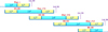Fig. 1 Time schedule for the daily computer runs at the Navigation Support Office to establish 48h time series of ZWDs and ZTDs, and tropospheric media calibrations.

Fig. 2 Ideal case A-matrix structure.

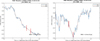Fig. 3 Examples of polynomial fitting in the case of data gaps, marked in red.

4 Ionospheric media calibrations

4.1 Ionospheric calibrations provided by JPL

Historically, ionospheric media calibrations processing at ESOC Flight Dynamics is aligned to JPL data formats, which may change in future. So the essentials of ionospheric calibrations provided by JPL (JPL, 2008) shall be summarized in the following for a better understanding of the own new approach, Section 4.2:

• specific for each station/spacecraft/frequency. − Upon need, ionospheric calibrations can be re-scaled to other frequencies very easily;

• ionospheric calibrations are computed per station for each tracking pass (from satellite rise to satellite set);

• per pass, the ionospheric calibrations are provided as line-of-sight corrections w.r.t. a reference frequency of 2295 MHz, which must be applied to the satellite ranging data;

• ionospheric calibrations are actually represented per pass in form of a polynomial as function of normalized time, Eq. (2). − Nevertheless, JPL has also the capability to provide multiple piecewise-continuous polynomials per pass;

• no background model, like the JPL Seasonal Model for the troposphere, is applied, i.e. the ionospheric polynomials provide absolute slant range delays;

• the user has to provide satellite trajectory information, giving the direction to the satellite as function of time, as input for the ionospheric calibrations computation. For delta-DOR observations, the quasar direction as function of time is required too.

4.2 Computation of ionospheric calibrations by the ESOC Navigation Support Office

As with the tropospheric calibrations, also for the ionospheric calibrations an approach has been worked out, which is based on own GNSS tracking data recorded and evaluated by the Navigation Support Office. This approach is simple, robust and easy to handle, relying as far as possible on in-house data and software and being as far as possible independent from external sources. − The only exception from this rule is the usage of the self-contained Neustrelitz TEC Model − Global (NTCM-GL) (Jakowski et al., 2011) for the computation of ionospheric background values.

The following input is required from the Navigation Support Office:

• GNSS data (RINEX) from the sites of the ESA DSN as well as from the global IGS network, including its preprocessing;

• GNSS satellite orbits and clocks from routine products generation for the IGS;

• sTEC and Differential Code Bias (DCB) values from routine ionosphere products generation for the IGS.

The following input is required from Flight Dynamics:

• ESA spacecraft/quasar trajectory information for the specified 48 hour time interval.

Interplanetary spacecraft/quasar passes never exceed 15 hours significantly. Thus per day an ionospheric media calibration is computed covering the 48-hours timespan from 0^h UT of today (observation day) back to 0^h UT of the day before yesterday. As with the troposphere, also ionosphere processing is conducted in rapid and in final mode. In rapid mode, this job is submitted via an automatic job scheduler (crontab) every day at 07:33 UT. In order to avoid short, truncated passes at the beginning and at the end of this 48-hours timespan, only those passes are considered which fall completely into the 48-hours interval. All other passes are considered in the jobs of the day before or after. The pass criterion is for a spacecraft/quasar to have an elevation angle of ≥5° at the considered station. Per day and ESA spacecraft/quasar, one CSP-file is generated covering all complete passes of this spacecraft/quasar at all considered stations for the last 48 hours from 0^h UT to 0^h UT. In final mode, the same processing is repeated at 07:03 UT, 4 days after the end of the observation day.

The developed method is based on the evaluation of dual-frequency GNSS data which is permanently recorded with receivers owned by the Navigation Support Office at numerous ESA tracking sites, among them the DSN sites CEBR, MGUE and NNOR. After preprocessing, series of uncalibrated sTEC values at each ESA DSN to all visible GNSS satellites over the specified 48-hours time interval are produced from the RINEX data. These sTEC values have to be corrected for the GNSS receiver and satellite DCBs (Schaer et al., 1998). The GNSS receiver and satellite DCBs are obtained from the global ionosphere model estimates conducted operationally each day at the Navigation Support Office, in which these DCBs are part of the estimation process. It should be noted that these DCBs cannot be estimated in an absolute sense so a certain reference (datum) has to be defined. This is done by specifying that the sum of the satellite DCBs is Zero. To avoid significant day-to-day variations in the DCB estimates, e.g. due to a missing satellite on a specific day changing the average, the daily DCB estimates of the last 7 days are combined. This smooths out the day-to-day variations and avoids jumps due to satellites missing on individual days, e.g. due to manoeuvres. It does, however, not resolve the change in the mean DCB level when a new satellite is added to the GNSS constellation.

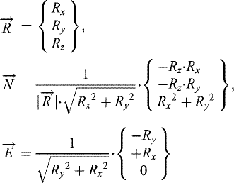
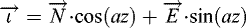
Then the algorithm works as follows per DSN station and ESA spacecraft/quasar: Per epoch, the unit vectors pointing from the station to all GNSS satellites and to the ESA spacecraft/quasar are simply computed from their position vectors (Fig. 4): 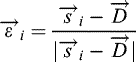$${{\displaystyle \overrightarrow{\epsilon }}}_i=\frac{{{\displaystyle \overrightarrow{s}}}_i-{\displaystyle \overrightarrow{D}}}{\left|{{\displaystyle \overrightarrow{s}}}_i-{\displaystyle \overrightarrow{D}}\right|}$$(6) where_{${{\displaystyle \overrightarrow{ϵ}}}_i$} – unit vector pointing from DSN site to spacecraft i;_{${{\displaystyle \overrightarrow{s}}}_i$} – geocentric earth-fixed position vector of spacecraft i (i = GNSS₁, GNSS₂, … GNSS_n, ESAspacecraft/quasar);

${\displaystyle \overrightarrow{D}}$ – geocentric position vector of DSN site.

Next, the cosines of the angles between all G_j = 1, …, n GNSS satellites and the ESA interplanetary spacecraft (ESA)/quasar (Q), as viewed from the DSN site, are computed: $$\cos {\mathit{\psi }}_{{\mathit{G}}_{\mathit{j}}\mathit{E}\mathit{S}\mathit{A}}={\overrightarrow{\mathit{\epsilon }}}_{{\mathit{G}}_{\mathit{j}}}·{\overrightarrow{\mathit{\epsilon }}}_{\mathit{E}\mathit{S}\mathit{A}}\mathrm{r}\mathrm{e}\mathrm{s}\mathrm{p}\mathrm{.}\cos {\mathit{\psi }}_{{\mathit{G}}_{\mathit{j}}\mathit{Q}}={\overrightarrow{\mathit{\epsilon }}}_{{\mathit{G}}_{\mathit{j}}}·{\overrightarrow{\mathit{\epsilon }}}_{\mathit{Q}}$$(7)

The smaller the angle between a GNSS satellite and the ESA spacecraft/quasar is, the closer its cosine value comes to +1, i.e. GNSS satellites viewed close to the ESA spacecraft/quasar will display cosine values near to +1, while far distant GNSS satellites will get cosine values close to −1, e.g. when both GNSS and ESA spacecraft/quasar are close to horizon but diametrical in direction (e.g. Fig. 6). Thus the 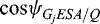$\cos {\psi }_{G_{j}ESA/Q}$ are well suited to establish a weighting when combining the GNSS sTEC values to a sTEC value into the direction of the ESA spacecraft/quasar. The following weighting function was selected for the ionospheric media calibrations: 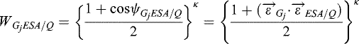$${\mathit{W}}_{{\mathit{G}}_{\mathit{j}}\mathit{E}\mathit{S}\mathit{A}/\mathit{Q}}={\left\{\frac{1+\cos {\mathit{\psi }}_{{\mathit{G}}_{\mathit{j}}\mathit{E}\mathit{S}\mathit{A}/\mathit{Q}}}{2}\right\}}^{\mathit{\kappa }}={\left\{\frac{1+({\overrightarrow{\mathit{\epsilon }}}_{{\mathit{G}}_{\mathit{j}}}·{\overrightarrow{\mathit{\epsilon }}}_{\mathit{E}\mathit{S}\mathit{A}/\mathit{Q}})}{2}\right\}}^{\mathit{\kappa }}$$(8)

i.e. $1\ge W_{G_{j}ESA/Q}\ge 0$ for $0^0\le {\psi }_{G_{j}ESA/Q}\le {180}^0$. With the power κ in Eq. (8) the distribution of weights might be further tuned. − Nevertheless, κ = 1 is used for the ionospheric calibrations.

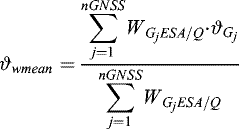
By introducing these weights, a weighted mean of the GNSS sTEC values, depending on the angular distances of the GNSS satellites from the ESA spacecraft/quasar, could principally be computed as: $$sTE{C}_{ESA/Q}=\frac{{\displaystyle \sum _{j=1}^{nGNSS}}{W}_{G_{j}ESA/Q}\cdot sTE{C}_{G_j}}{{\displaystyle \sum _{j=1}^{nGNSS}}{W}_{G_{j}ESA/Q}}$$(9)

Tests, however, showed that Eq. (9) does not provide satisfactory sTEC values into ESA spacecraft/quasar direction. The above principal approach, Eqs. (6)–(9), had thus to be improved and supplemented by the following measures in order to meet anticipated accuracy margins:

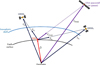Fig. 4 Considered vector geometry between DSN station, GNSS satellites and ESA spacecraft/quasar.

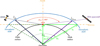Fig. 6 Maximal possible geocentric angle ξmax for given mean earth radius RM and ionospheric shell height hI.

4.2.1 Measure 1

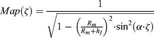
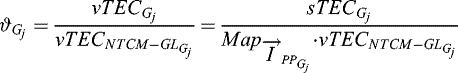
An alternative to directly processing the sTEC values, is to map them with a mapping function, Eq. (10), into the vertical in order to compute the weighted mean vTEC and then to map this weighted mean vTEC back into the slant range direction of the ESA spacecraft/quasar: $$Map\left(\zeta \right)=\frac{1}{\sqrt{1-{\left(\frac{R_m}{R_m+h_I}\right)}^2\cdot {\sin }^2\left(\alpha \cdot \zeta \right)}}$$(10) whereζ = 90⁰ − el – zenith distance at ionospheric shell of maximum ionization (IPP, Appendix A).${\mathit{R}}_{\mathit{m}}=6371\mathrm{k}\mathrm{m},{\mathit{h}}_{\mathit{I}}=450\mathrm{k}\mathrm{m},\mathit{\alpha }=1$ Standard Mapping Function, IONEX and NTCM-GL;${\mathit{R}}_{\mathit{m}}=6371\mathrm{k}\mathrm{m},{\mathit{h}}_{\mathit{I}}=506.7\mathrm{k}\mathrm{m},\mathit{\alpha }=0.9782$ Modified Single Layer Model Mapping Function.

Depending on parameters (R_M, h_I, α) setting, Eq. (10) can either be evaluated as the Standard Mapping Function, or as the Modified Single Layer Model Mapping Function (MSLM, ftp://ftp.unibe.ch/aiub/users/schaer/igsiono/doc/mslm.pdf) (Schaer, 1999). The MSLM is an optimal fit to the extended slab model mapping function used by JPL (Mannucci et al., 1998; Coster et al., 1992).

The relation between sTEC and vTEC is then: $$STEC=Map\left(\zeta \right)\cdot VTEC$$(11)

With Eq. (11) the weighted mean of the vTEC can be expressed in terms of sTEC and mapping function, by modifying Eq. (9): $$vTE{C}_{ESA/Q}=\frac{{\displaystyle \sum _{j=1}^{nGNSS}}{W}_{G_{j}ESA/Q}\cdot vTE{C}_{G_j}}{{\displaystyle \sum _{j=1}^{nGNSS}}{W}_{G_{j}ESA/Q}}\Rightarrow \frac{sTE{C}_{ESA/Q}}{Map\left({\zeta }_{ESA/Q}\right)}=\frac{{\displaystyle \sum _{j=1}^{nGNSS}}{W}_{G_{j}ESA/Q}\cdot \frac{sTE{C}_{G_j}}{Map\left({\zeta }_{G_j}\right)}}{{\displaystyle \sum _{j=1}^{nGNSS}}{W}_{G_{j}ESA/Q}}$$(12)

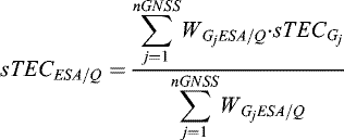
By solving Eq. (12) for sTEC_ESA/Q and introducing Eq. (10) for the mapping functions, one obtains after the some algebra the following formulation: $$sTE{C}_{ESA/Q}=\frac{1}{\sqrt{C+{\left\{R_m\cdot \cos \left(\alpha \cdot {\zeta }_{ESA/Q}\right)\right\}}^{\mathrm{}}{}^2}}\cdot \left\{\frac{{\displaystyle \sum _{j=1}^{nGNSS}}{W}_{G_{j}ESA/Q}\cdot sTE{C}_{G_j}\cdot \sqrt{C+{\left\{R_m\cdot \cos \left(\alpha \cdot {\zeta }_{G_j}\right)\right\}}^{\mathrm{}}{}^2}}{{\displaystyle \sum _{j=1}^{nGNSS}}{W}_{G_{j}ESA/Q}}\right\}$$(13) where

C = h_I ⋅ (2 ⋅ R_m + h_I) – auxiliary constant.

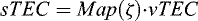
The zenith distances ζ_ESA/Q,Gj required in Eq. (13) have to be computed at the IPP positions, where the slant ranges to the ESA spacecraft/quasar and to the GNSS satellites intersect the ionospheric shell of maximum ionization h_I. The computation of the IPP position vectors is described in Appendix A, whereby here the unit vector pointing into range direction is already known, Eq. (6), and must not be first computed from azimuth and elevation, i.e. the calculations can enter directly at Eq. (A.4) into the Appendix A algorithm. With these IPP position vectors, the required cosines of the zenith distances are evaluated: $$\cos {\zeta }_{ESA/Q}={{\displaystyle \overrightarrow{\epsilon }}}_{ESA/Q}\cdot \frac{{{\displaystyle \overrightarrow{I}}}_{P{P}_{ESA/Q}}}{\left(R_m+h_I\right)}\text{\hspace{0.17em} and \hspace{0.17em}}\cos {\zeta }_{G_j}={{\displaystyle \overrightarrow{\epsilon }}}_{G_j}\cdot \frac{{{\displaystyle \overrightarrow{I}}}_{P{P}_{G_j}}}{\left(R_m+h_I\right)}$$(14) where R_m – mean earth radius, for values see Eq. (10);h_I – ionospheric shell height, for values see Eq. (10).

4.2.2 Measure 2

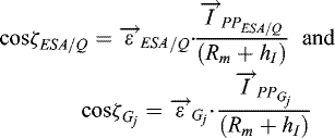
When inspecting Figure 5 it becomes obvious that the angular distances between the ESA spacecraft/quasar and the GNSS satellites, as viewed from the station, can provide a rather distorted picture of the local ionosphere above, whose principal layered structure is indicated in Figure 5 by its shell of maximum ionization at altitude h_I. So appears GNSS₂ seen from the station much closer to the ESA spacecraft/quasar than the angular distance between the IPP position vectors of both would justify. Thus a probably higher weight is appointed to GNSS₂ as it in reality would deserve. In order to achieve a more objective weighting, the angular distances ξ between the IPP position vectors (green in Fig. 5) should be computed and enter into the weight computation, rather than the angular distances ψ as viewed from the station (red in Fig. 5). So Eq. (7) is modified to: $$\cos {\xi }_{G_j\mathit{E}\mathit{S}\mathit{A}}=\left(\frac{{{\displaystyle \overrightarrow{I}}}_{P{P}_{G_j}}}{\left|{{\displaystyle \overrightarrow{I}}}_{P{P}_{G_j}}\right|}\cdot \frac{{{\displaystyle \overrightarrow{I}}}_{P{P}_{ESA}}}{\left|{{\displaystyle \overrightarrow{I}}}_{P{P}_{ESA}}\right|}\right)\mathrm{r}\mathrm{e}\mathrm{s}\mathrm{p}\mathrm{.}\cos {\xi }_{G_j\mathit{Q}}=\left(\frac{{{\displaystyle \overrightarrow{I}}}_{P{P}_{G_j}}}{\left|{{\displaystyle \overrightarrow{I}}}_{P{P}_{G_j}}\right|}\cdot \frac{{{\displaystyle \overrightarrow{I}}}_{P{P}_Q}}{\left|{{\displaystyle \overrightarrow{I}}}_{P{P}_Q}\right|}\right)$$(15)

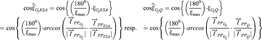
Before the cosine values obtained with Eq. (15) are entered into Eq. (8) for weight computation, their value range should be increased. While the angular distances ψ, as viewed from the station (red in Figs. 5 and 6), can achieve values between 0° ≤ ψ ≤ 180° (180° when both GNSS satellite and ESA spacecraft/quasar appear at the tracking site close to horizon, but almost diametrical in direction), the angular distances ξ between the IPP position vectors (green in Figs. 5 and 6) can get maximum values of 0° ≤ ξ ≤ ξ_max ≈ 40° only (Fig. 6). This angular range limitation of ξ will also reduce the range of cosine values for weight computation by Eq. (8) considerably. In order to achieve a wider range of angular arguments for the cosine function and thus a better weighting, the ξ are artificially enlarged as follows: 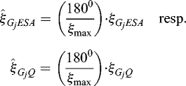$${{\displaystyle \hat{\xi }}}_{G_{j}ESA}=\left(\frac{{180}^0}{{\xi }_{\max }}\right)\cdot {\xi }_{G_{j}ESA}\mathrm{r}\mathrm{e}\mathrm{s}\mathrm{p}\mathrm{.}{{\displaystyle \hat{\xi }}}_{G_{j}Q}=\left(\frac{{180}^0}{{\xi }_{\max }}\right)\cdot {\xi }_{G_{j}Q}$$(16)

Instead of the cosine values obtained from Eq. (15), the following cosine values should then enter into Eq. (8) for weight computation, based on Eq. (16): $$\begin{array}{cc}\cos {{\displaystyle \hat{\xi }}}_{G_{j}ESA}=\cos \left\{\left(\frac{{180}^0}{{\xi }_{\max }}\right)\cdot {\xi }_{G_{j}ESA}\right\}& \cos {{\displaystyle \hat{\xi }}}_{G_{j}Q}=\cos \left\{\left(\frac{{180}^0}{{\xi }_{\max }}\right)\cdot {\xi }_{G_{j}Q}\right\}\\ =\cos \left\{\left(\frac{{180}^0}{{\xi }_{\max }}\right)\cdot \arccos \left(\frac{{{\displaystyle \overrightarrow{I}}}_{P{P}_{G_j}}}{\left|{{\displaystyle \overrightarrow{I}}}_{P{P}_{G_j}}\right|}\cdot \frac{{{\displaystyle \overrightarrow{I}}}_{P{P}_{ESA}}}{\left|{{\displaystyle \overrightarrow{I}}}_{P{P}_{ESA}}\right|}\right)\right\}\mathrm{r}\mathrm{e}\mathrm{s}\mathrm{p}\mathrm{.}& =\cos \left\{\left(\frac{{180}^0}{{\xi }_{\max }}\right)\cdot \arccos \left(\frac{{{\displaystyle \overrightarrow{I}}}_{P{P}_{G_j}}}{\left|{{\displaystyle \overrightarrow{I}}}_{P{P}_{G_j}}\right|}\cdot \frac{{{\displaystyle \overrightarrow{I}}}_{P{P}_Q}}{\left|{{\displaystyle \overrightarrow{I}}}_{P{P}_Q}\right|}\right)\right\}\end{array}$$(17) where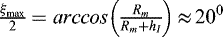$\frac{{\xi }_{\max }}{2}=\arccos \left(\frac{R_m}{R_m+h_I}\right)\approx {20}^0$ (Fig. 6, green triangles).

Fig. 5 Computing weights from the angles enclosed by the IPP position vectors.

4.2.3 Measure 3

The weighted mean sTEC value computed with Eq. (13) (considering Eqs. (15) and (17)) does represent the sTEC in the direction to the ESA spacecraft/quasar only with limited accuracy and is “corrected” with the aid of the NTCM-GL background model as follows: $${\displaystyle \tilde{s}}TE{C}_{ESA/Q}=sTE{C}_{ESA/Q}+{\vartheta }_{wmean}\cdot Ma{p}_{{{\displaystyle \overrightarrow{I}}}_{P{P}_{ESA/Q}}}\cdot \left(vTE{C}_{NTCM-G{L}_{ESA/Q}}-vTE{C}_{NTCM-G{L}_{wmean}}\right)$$(18a)

The right hand side of Eq. (18a) comprises the following parameters:

• Weighted mean TEC ratio between actual level of ionization and NTCM-GL background level:

$${\vartheta }_{wmean}=\frac{{\displaystyle \sum _{j=1}^{nGNSS}}{W}_{G_{j}ESA/Q}\cdot {\vartheta }_{G_j}}{{\displaystyle \sum _{j=1}^{nGNSS}}{W}_{G_{j}ESA/Q}}$$(18b)

• TEC ratio between actual level of ionization and NTCM-GL background level at the j-th GNSS satellite:

$${\vartheta }_{G_j}=\frac{vTE{C}_{G_j}}{vTE{C}_{NTCM-G{L}_{G_j}}}=\frac{sTE{C}_{G_j}}{Ma{p}_{{{\displaystyle \overrightarrow{I}}}_{P{P}_{G_j}}}\cdot vTE{C}_{NTCM-G{L}_{G_j}}}$$(18c)

• $Ma{p}_{{{\displaystyle \overrightarrow{I}}}_{P{P}_{ESA/Q}}}$… mapping function value, Eq. (10), evaluated at ESA spacecraft/quasar IPP location;

• $Ma{p}_{{{\displaystyle \overrightarrow{I}}}_{P{P}_{G_j}}}$ … mapping function value, Eq. (10), evaluated at j-th GNSS IPP location;

• $sTE{C}_{G_j}$ … sTEC measured by j-th GNSS satellite, appearing also in Eq. (9);

• $vTE{C}_{G_j}$ … vTEC corresponding to measured $sTE{C}_{G_j}$;

• $vTE{C}_{NTCM-G{L}_{G_j}}$ … NTCM-GL vTEC computed at j-th GNSS IPP location;

• $vTE{C}_{NTCM-G{L}_{ESA/Q}}$ … NTCM-GL vTEC computed at ESA spacecraft/quasar IPP location;

• $vTE{C}_{NTCM-G{L}_{wmean}}$ … NTCM-GL vTEC computed at weighted mean IPP location, Eq. (18d);

• Unit vector pointing from ground station into the direction of weighted mean sTEC, Eq. (13), component-wise mean of GNSS range unit vectors:

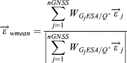$${{\displaystyle \overrightarrow{ϵ}}}_{wmean}=\frac{{\displaystyle \sum _{j=1}^{nGNSS}}{W}_{G_{j}ESA/Q}\cdot {{\displaystyle \overrightarrow{ϵ}}}_j}{\left|{\displaystyle \sum _{j=1}^{nGNSS}}{W}_{G_{j}ESA/Q}\cdot {{\displaystyle \overrightarrow{ϵ}}}_j\right|}$$(18d)

The unit vectors ${{\displaystyle \overrightarrow{ϵ}}}_j$ pointing from ground station to the j GNSS satellites were computed with Eq. (6). ${{\displaystyle \overrightarrow{ϵ}}}_{wmean}$ is needed to compute the IPP location ${{\displaystyle \overrightarrow{I}}}_{wmean}$, Appendix A, corresponding to the weighted mean sTEC. At this IPP, a NTCM-GL vTEC value has to be computed too for Eq. (18a).

In summary, NTCM-GL vTEC values need to be computed for Eq. (18a) at the IPPs of the ESA spacecraft/quasar, all GNSS satellites and the weighted mean sTEC direction.

Equation (18a) can be summarized as follows: The weighted mean sTEC, as obtained from Eq. (13) (considering Eqs. (15) and (17)), is corrected for a sTEC offset between the IPP location of the ESA interplanetary spacecraft/quasar direction and the IPP corresponding to the direction of the weighted mean over all GNSS satellite directions involved. This offset is computed as NTCM-GL vTEC difference between the ESA spacecraft/quasar IPP location and the IPP location of the weighted mean sTEC direction, mapped into the slant range at the ESA spacecraft/quasar IPP location. By the difference making, potential biases between the NTCM-GL and measured GNSS sTEC observables cancel. To account for the actual ionospheric activity level, corresponding to the actual ionospheric overall charge w.r.t. the NTCM-GL background level, at the IPP position of each GNSS satellite a background TEC value is computed with the NTCM-GL too and set in ratio to the actually measured sTEC at that IPP, Eq. (18c). The vTEC difference, ESA spacecraft/quasar IPP minus weighted mean sTEC IPP, is then scaled by the weighted mean ratio, Eq. (18b), to account for the actual ionization level w.r.t. the ionization level represented by the NTCM-GL. As closer as the IPP positions into ESA interplanetary spacecraft/quasar direction and of the weighted mean sTEC coincide, as closer this difference will approach Zero, and finally vanish in case of coincidence. In addition, by applying this correction, also the situation of unfavourable geometrical conditions will be mitigated, e.g. in case that an ESA spacecraft/quasar is not surrounded by directions to GNSS satellites. − Normally this should not happen, since interplanetary missions are typically located in − or close to the ecliptic plane, a region which is well covered by the GNSS constellations. Measure 3 included _ see Figure 11a

Figure 7 shall illustrate how the weighted mean sTEC values (red & violet curves) approach closer and closer the sTEC curve of an excluded GNSS satellite (blue), which served as reference, by introducing in sequence Measure 1–3, whereby the final curve (Measure 3) is shown in Figure 11a. A description of the figure details and all curves displayed and their meaning is also provided beneath Figure 11.

Theoretically, Eqs. (6)–(18) could also work with only one GNSS satellite. Of course the algorithm will in practice not be applied in this way, but this indicates that it is very robust and stable, and thus well suited for operational use. As an indicator of quality for the interpolated sTEC value into ESA interplanetary spacecraft/quasar direction, the following additional parameter can be evaluated, in parallel to the weighted mean: 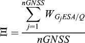$$\mathrm{\Xi }=\frac{{\displaystyle \sum _{j=1}^{nGNSS}}{W}_{G_{j}ESA/Q}}{nGNSS}$$(19)

Ξ is something like a “mean” of the weights of all GNSS satellites, based on Eq. (8). Ξ ≈ 1 would indicate a close angular distance of most of the GNSS satellites to the ESA spacecraft/quasar, Ξ ≈ 0.5 medium angular distance and Ξ ≈ 0 far angular distance, i.e. the closer Ξ comes to One, the better the sTEC value for the ESA spacecraft/quasar could be determined.

The angle between ESA spacecraft/quasar and weighted mean sTEC direction, either in terms of range from station (Eq. (20) top) or in terms of IPPs (Eq. (20) bottom), can serve as additional accuracy measure: $$\begin{array}{ccc}\hfill \cos \varsigma =\left(\frac{{{\displaystyle \overrightarrow{I}}}_{P{P}_{ESA/Q}}}{\left|{{\displaystyle \overrightarrow{I}}}_{P{P}_{ESA/Q}}\right|}\cdot \frac{{{\displaystyle \overrightarrow{I}}}_{wmean}}{\left|{{\displaystyle \overrightarrow{I}}}_{wmean}\right|}\right)\hfill & \hfill \to \hfill & \hfill 1\hfill \end{array}\mathrm{r}\mathrm{e}\mathrm{s}\mathrm{p}\mathrm{.}\begin{array}{ccc}\hfill \cos \theta ={{\displaystyle \overrightarrow{\epsilon }}}_{ESA/Q}\cdot {{\displaystyle \overrightarrow{\epsilon }}}_{wmean}\hfill & \hfill \to \hfill & \hfill 1\hfill \end{array}$$(20)

The angle enclosed by ESA spacecraft/quasar direction and sTEC weighted mean direction should be preferably close to Zero and its cosine value should approach One.

In the case of non-availability of GNSS observation data and/or systems, Flight Dynamics will compute ionospheric corrections with the NTCM-GL.

For the ionospheric CSP-files writing, the computed sTEC values along an ESA interplanetary spacecraft/quasar pass are then expressed in terms of group delays (e.g. Davies, 1990; Komjathy, 1997) w.r.t. to a reference frequency of 2295 MHz. This frequency was selected to be consistent with the current processing system set up at Flight Dynamics. $$g{}_{ion}=\frac{+40.3}{f^2}\cdot sTEC$$(21) whereg_ion – ionospheric code group delay [m];40.3 – constant originating from the Appleton-Hartree refractive index formula [m³/s²];f – satellite signal frequency [Hz], here set to 2295 × 10⁶ Hz (re-scaling to group delays at another frequency f by multiplication with {2295 × 10⁶ Hz/f}²);sTEC – total electron content along the signal's slant range path through the ionosphere [m⁻²];

Finally, a normalized-time polynomial of degree Five, Eq. (2), is fitted to this sTEC series of ionospheric slant range delays. One polynomial is fitted per pass. Per day and ESA spacecraft/quasar, one CSP-file is produced covering all complete passes of this spacecraft/quasar at all considered stations for the last 48 hours from 0^h UT to 0^h UT.

An implementation of media calibration extrapolations has so far not been considered and is not planned for the time being.

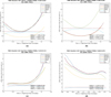Fig. 11 (a) Example from Test Case 1; (b) example from Test Case 1 with sTEC simulated by NTCM-GL; (c) example from Test Case 2; (d) example from Test Case 3.

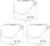Fig. 7 (a) Computing sTECESA/Q only with Eqs. (6)–(9); (b) Measure 1 included; (c) Measure 2 included; (d) Measure 3 included → see Figure 11a.

5 Results

5.1 Tropospheric media calibrations

The tropospheric media calibrations were validated by analysing orbit determination statistics obtained when using the media calibrations derived from the Saastamoinen (1973) Model on one hand and when using the media calibrations computed with the approach described in Section 3 on the other. The Saastamoinen Model employed for the comparison makes use of real weather data collected at the stations, and includes both the wet and dry components of the tropospheric zenith delay. The Niell Mapping Function (Niell, 1996, 2000) is used in both cases to map the zenith delays to the desired elevation.

Figure 8 shows an example of a fitted 8 × 6^h polynomial sequence for the dry part (Fig. 8a) and for the wet part (Fig. 8b). The station in Fig. 8 exemplary case is MGUE. The blue noisy curves display the δTZDs derived from GNSS observables, the red curves the sequence of fitted polynomials. Only the four central polynomials of the 8 × 6^h sequence enter then into the CSP file of the respective day (blue in Fig. 1). Table 1 summarizes the RMS values obtained on the example day of Figure 8 (12 April 2016, 12:00 – 14 April 2016, 12:00; 16.104–16.105 in the plot headers indicate the time range for the central 24^h in YY.DDD) for all three ESA DSN sites. The RMS values were computed from the differences of GNSS-derived δTZD minus computed polynomial value. A 15^m time resolution in the SINEX.tro file lead to 97 tropospheric zenith delay samples in the considered 48^h time interval.

In the following, the validation results for the new corrections used within the orbit determination of deep-space probes are presented. Statistics of orbit determinations (OD) made by using the tropospheric media calibrations computed with the approach described in Section 3 (called TRCal in the following) were compared with corresponding statistics when the tropospheric media calibrations from the legacy Saastamoinen Model were employed. For all the test cases presented for the validation of tropospheric corrections, the ionospheric delay is treated by the means of the NTCM-GL model.

Two test scenarios, based on GAIA and LISA pathfinder routine orbit determination, have been used. Both satellites are orbiting in a very quiet dynamic environment, better suited for observation models comparison compared to planetary orbiters. The configuration of the OD is briefly summarised in the following paragraphs. For more details on deep space OD terminology and ESOC OD software refer to Moyer (1971, 2000) and Budnik et al. (2004).

• GAIA: The spacecraft is orbiting in proximity of the Sun-Earth libration point L2, thus is mainly tracked during local evening, night or early morning. GAIA is extensively tracked from all of the ESA DSN stations, providing a very good test case for atmospheric delays validation. A data arc of three weeks duration (07 – 28 March 2017) has been selected for the orbit determination. Up to three Doppler passes per day are available from all ESA deep space stations, while, due to mission constraints, only a single ranging session per day is possible, split into two 10-minutes periods at the beginning and the end of all NNOR passes. No station keeping manoeuvres were present in the chosen period, however some dynamic parameters needed to be estimated such as the corrections to the Solar Radiation Pressure (SRP) model and to the propulsion model, given that GAIA attitude is controlled with low-thrust propulsion. GAIA is always tracked at elevations higher than 10°. The Doppler measurements are compressed to one-minute count intervals, and the frequency of range measurements, when available, is one data point per minute. More details about GAIA orbit determination can be found in Budnik et al. (2012);

• LISA Pathfinder: The satellite is orbiting in proximity of the Sun-Earth libration point L1, and is tracked by a single ESA station at Cebreros, mostly during local morning and daytime for a total duration of 8 hours per day, during which both Doppler and range measurements are continuously acquired. For this scenario a data arc of 18 days duration was used (13 Feb. − 03 Mar. 2017). LISA pathfinder is tracked with elevation down to 6°, which poses a major challenge in terms of tropospheric corrections. Due to this reason, for every type of calibration employed two runs were made, the first including all data and the second including only data at elevations higher than 10°. Also for this test case, the Doppler measurements are compressed with one-minute count intervals, while range measurements are sampled every 10 minutes. The dynamic parameters estimated in the orbit determination include only the satellite state vector and the corrections for the internal gravity between the satellite and the test masses used to control the force-free motion of the satellite (Armano et al., 2016).

For both scenarios, the orbit determination has been performed with the ESOC operational orbit determination software AMFIN (Budnik et al., 2004). A range bias per pass is estimated in the fit to compensate for time dependent unmodelled effects. The a-posteriori dispersion of the range biases is usually a good indicator of possible systematic errors in both the dynamics and the   observations modelling, and of possible radial errors in the reconstructed trajectory.

The reported statistics include the overall RMS of all Doppler and range residuals, intended as the measured minus computed values of the observations based on the estimated solution (trajectory plus estimated parameters). The dispersion, in terms of RMS, of the estimated range biases is also included.

Figure 9 gives an overview of the evolution of the Doppler residuals over the entire data arc used for the GAIA OD, in this case with tropospheric corrections derived from TRCal. In Table 2 the statistics of the observation residuals are compared between the two calibration methods. It can be seen that all the figures present a noticeable improvement when passing from the Saastamoinen-based corrections to the TRCal ones. Even though the Doppler residuals RMS is dominated by the presence of some very noisy passes, likely due to high solar/geomagnetic activity, the benefit of GNSS-based corrections can be appreciated especially when the satellite is tracked at low elevation. In Figure 10, some tails at the beginning and the end of the passes, i.e. at low elevation, are visible in the Doppler residuals when the Saastamoinen Model is used (top plot), while they disappear when the TRCal are used (bottom plot). These tails are typical for a systematic error in the tropospheric zenith delays over relatively long time periods (tens of minutes to hours) mapped down to low elevation, and they can have a larger impact on the OD accuracy than a plain uncoloured noise of even larger amplitude like the one visible in some passes in Figure 9.

Table 3 reports the comparison of LISA Pathfinder orbit determination statistics. Also in this case the statistics on the range biases and Doppler residuals improve when the new GNSS based calibrations are employed. In particular, the Doppler residuals show a significant improvement (more than 10%) when the data at low elevation is included in the OD. The RMS of the range residuals does not show a noticeable improvement when changing the calibration method. This could be a consequence of the larger background noise, compared to the GAIA case, possibly masking small variations in the residuals.

On top of the formal validation of the operational tropospheric calibrations presented here, the corrections generated in pre-operational mode were used successfully for over one year for GAIA routine orbit determination.

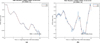Fig. 8 (a) Example of dry-part polynomials; (b) example of wet-part polynomials.

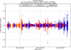Fig. 9 Overview of Doppler residuals over the full arc used in the GAIA OD; tropospheric corrections based on TRCal.

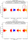Fig. 10 Comparison of 2-way Doppler residuals with Saastamoinen (top plot) and TRCal (bottom plot) corrections.

5.2 Ionospheric media calibrations

The ionospheric media calibrations were validated by two basic methods:

• The ESA spacecraft/quasar was replaced by a GNSS satellite, whose sTEC values are known from its dual-frequency measurements. These measured sTEC values were then compared with the weighted mean sTEC derived from the dual-frequency data of all the other GNSS satellites, Section 4. In addition, corresponding sTEC values were interpolated from JPL IONEX files along the excluded GNSS satellite's trajectory, as well as computed with the NTCM-GL;

• An analysis of orbit determination statistics obtained by using media calibrations based on the legacy NTCM-GL model on one hand and by using the media calibrations computed with the new approach, as described in Section 4, on the other.

5.2.1 Validation method 1

Figure 11 stands exemplarily for the results of a systematic validation of the ionospheric calibrations, that were conducted by replacing the ESA spacecraft/quasar with a GNSS satellite excluded from the polynomials computation and whose measured sTEC values served then as reference for the weighted mean sTEC values computed from the measurement data of all the other GNSS satellites, Eqs. (6)–(18). Three test cases were considered:

• Test Case 1: 19 July 2015, 00:00 − 21 July 2015, 00:00, normal ionospheric conditions;

• Test Case 2: 8 May 2016, 00:00 − 10 May 2016, 00:00, strong magnetic storm with Kp values up to 7 (the planetary K-index, Kp, is a measure for the irregular variations of the Cartesian components of the geomagnetic field and is used to characterize geomagnetic storms, e.g. Komjathy (1997) and http://www.swpc.noaa.gov/products/planetary-k-index);

• Test Case 3: 8 March 2016, 00:00 − 10 March 2016, 00:00, solar eclipse over the Pacific (http://www.timeanddate.com/eclipse/solar/2016-march-9) which was at least partly visible from NNOR.

Per test case, five GNSS satellites, GPS as well as GLONASS, were arbitrarily chosen to serve in sequence as reference for the validation. For Test Case 3, GNSS satellites that were affected by the solar eclipse had been selected. Then per excluded GNSS satellite and pass/arc of that satellite, a CSP-file was computed from the data of all the other GNSS satellites and the weighted mean sTEC values were then compared with the sTEC series measured by the excluded GNSS satellite. Per test case, about 70 passes/arcs at the three ESA DSN sites CEBR, MGUE, NNOR were evaluated. Figure 11 shows examples of the coincidence between the curves resulting from different sources to compute the ionospheric media calibrations for the three test cases.

Figure 11 displays the slant range corrections [m] w.r.t. to a 2295 MHz reference frequency, Eq. (21), in the following colours:

• Blue: Measured sTEC of the excluded GNSS satellite serving as reference;

• Red: Weighted mean sTEC obtained from the other GNSS satellites (noisy curve), Eq. (18);

• Violet: sTEC values computed from the CSP polynomial (this is always a smoothed version of the red weighted mean curve, the polynomial degree is 5);

• Green: sTEC interpolated from a JPL IONEX file along the excluded GNSS satellite's trajectory;

• Yellow: sTEC computed with the NTCM-GL along the excluded GNSS satellite's trajectory;

• Brown: cosθ, cosς, Eq. (20), should always be close to One;

• Pale blue: Ξ-parameter, Eq. (19), should always be close to One.

In addition, Figure 11 presents the RMS values of differences:

• RMSg-w: measured sTEC of excluded GNSS satellite minus weighted mean sTEC;

• RMSg-j: measured sTEC of excluded GNSS satellite minus interpolated JPL IONEX sTEC;

• RMSw-j: weighted mean sTEC minus interpolated JPL IONEX sTEC.

The following aspects should be kept in mind when inspecting Figure 11:

• the JPL IONEX files include always all available GNSS satellites, i.e. also the one selected in the analysis as reference;

• what the blue curve (reference GNSS satellite) displays, are measurements too, i.e. also the reference sTEC values are subject to noise and inaccuracies;

• the red weighted mean curve (then smoothed by the polynomial fit, violet CSP curve) and the pale blue Ξ-curve display noisy behaviour. Since the weighting method is purely geometric-based, this noise may be induced by changing GNSS constellations (some satellites rise, while other set);

• the analysis follows here the trajectory of the excluded GNSS satellite. While interplanetary missions are typically located in − and around the ecliptic, GNSS satellites can achieve considerably higher latitudes (GPS 55°, GLONASS 64°.8, Galileo 56°).

Figures 11a, c, d show the different curves for sTEC values derived from measured data; the only exception here is the NTCM-GL curve (yellow). A systematic shift of the NTCM-GL curve w.r.t. the other GNSS measurements-based curves is clearly visible. This “bias” reflects the difference of the actual ionisation level w.r.t. a background ionisation level represented by the NTCM-GL.

Figure 11b shows for the same pass/arc of Figure 11a the situation when all measured sTEC values were “simulated” with the NTCM-GL. Only the JPL IONEX curve remains measurements-based; this could not be changed. Now the measurements-based green JPL curve displays nicely the offset between the actual level of ionospheric ionisation and the background ionisation level represented by the NTCM-GL. Since here also the reference sTEC values were simulated with the NTCM-GL, the blue curve is in this special case always identical with the yellow curve and thus not visible (the RMS values displayed in Figure 11b are meaningless). The analysis by taking NTCM-GL simulated sTEC values as “observables” seems to confirm that the weighted mean sTEC method, as described in Section 4, works principally.

In order to get a more detailed picture about the overall performance of the new weighted mean sTEC method versus JPL, the three types of RMS values, displayed in Figure 11 (not Fig. 11b), were analysed for all considered passes/arcs and the three test cases in the form of histograms (Fig. 12). In Figure 12 the RMS types RMSg-w, RMSg-j and RMSw-j (from left to right) of all passes/arcs (≈70 per test case) are shown in the form of histograms for each of the three test cases (from top to down). Since RMS values are naturally always positive, the resulting histograms comprise only the positive part of the abscissa. In the ideal case, the majority of RMS values should be small; thus the resulting histograms should display a peak close to the ordinate and then decay to the right along the abscissa. The strength of that decay and the height, location and width of the peak are an indicator on how good the media calibrations were able to reproduce the reference sTEC values of the excluded GNSS satellite under the different ionospheric conditions of the three test cases.

In addition to the histograms, Table 4 summarizes the mean, standard deviation, minimal and maximal RMS values of the different RMS types for the three test cases.

When inspecting Figure 12 and Table 4, one can come to the following conclusions:

• under normal ionospheric conditions, Test Case 1, the overall distribution of the RMSg-w values (weighted mean sTEC, red histogram) and the RMSg-j values (JPL, green histogram) are of comparable shape. The RMSw-j values (brown histogram) summarize then the differences between weighted mean sTEC and JPL IONEX-derived sTEC. Smaller values for the mean (peak position) and the standard deviation (width) of the RMSg-w values compared to the RMSg-j values indicate a slightly better performance of the new weighted mean sTEC approach over the JPL IONEX-derived sTEC numbers. The range of maxima and minima is of the same magnitude for both the RMSg-w values and the RMSg-j values;

• under strong magnetic storm conditions, Test Case 2, mean and standard deviation are slightly smaller for the RMSg-w values (weighted mean sTEC, red histogram) compared to the RMSg-j values (JPL, green histogram) too. Also the range of outliers, indicated by the maxima and minima, is smaller for the RMSg-w values than for the RMSg-j values. Thus for Test Case 2, the RMSg-w values are slightly favourite over the RMSg-j values too;

• during the solar eclipse, Test Case 3, mean and standard deviation of the RMSg-w values (weighted mean sTEC, red histogram) are clearly smaller than for the RMSg-j values (JPL, green histogram). On the other hand, Table 4 shows that the spread between maxima and minima is larger for the RMSg-w values compared to the RMSg-j values;

• in all cases the RMSg-j values (JPL, green histograms) seem to display more sensitivity to outliers (higher bars on the right part of the abscissa in Fig. 12) than the RMSg-w values (weighted mean sTEC red histograms).

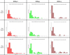Fig. 12 Histogram analysis of RMS values.

5.2.1.1 Summary of validation method 1

The ionospheric media calibrations computed with the new weighted mean sTEC method, Section 4, seem to display a slightly better performance compared to the JPL IONEX data. As pointed out above, the reference GNSS satellite could not be excluded from the JPL data, in this way slightly favouring the JPL data. And as pointed out above too, the sTEC values from the reference GNSS satellite were also measurements subjected to noise and errors, i.e. they were not absolute. So in summary, the weighted mean sTEC media calibrations compare favourably to those computed from the JPL IONEX files.

5.2.2 Validation method 2

For the validation of the ionospheric calibrations in the context of a deep-space satellite orbit determination (OD), the same procedure and the same scenarios were used as the ones described in Section 5.1.

The legacy model for the ionospheric corrections is the NTCM-GL (Jakowski et al., 2011), which was implemented in recent years and demonstrated to reliably improve the quality of the orbit determination compared to the previously used Klobuchar model (Klobuchar, 1975). This model is here compared in terms of OD statistics with the calibrations based on the approach described in Section 4, called IOCal in the following.

The effect of the ionospheric delay on range and Doppler observations is less pronounced than the tropospheric one for X-band satellites. The best available corrections for troposphere, i.e. the ones based on GNSS, need to be used in order to reduce the overall noise level of the tracking data and make the comparison of orbit determination statistics easier. For the same reason, for the LISA Pathfinder scenario only the test case with elevation larger than 10° was kept for this assessment.

In Table 5 the residuals and range bias statistics are reported for the GAIA scenario. It can be observed that no significant change is visible in terms of range and Doppler residuals; however, the range bias RMS increases by a factor two compared with the legacy model. This might indicate that some systematic source of error could still be present in the IOCal corrections. The reconstructed orbits differ by up to 450 m, which is in line with the formal uncertainty of the OD solution based on range and Doppler at declination lower than 10° (Budnik et al., 2012).

To better understand this somehow unexpected result, a dedicated investigation was carried out, which exposed some issues at the level of pre-processing the GNSS data, like an inter-system bias between the GPS and GLONASS constellation that was not properly accounted for. The results reported in this section already take into account the updated calibrations, that are in general more consistent with other sources of data and models compared to the initial runs, but still do not improve in a significant way the quality of the orbit determination. Further improvements at pre-processing level have already been identified, which require longer-term developments that cannot be incorporated in this paper results.

Table 6 shows the comparison of the OD statistics for the LISA Pathfinder test case. A minor but insignificant improvement can be observed for this scenario in the Doppler residuals as well as in the range biases, although its magnitude is essentially within the level of noise of the measurements. The two solutions can be considered equivalent both in terms of statistics and orbit, with a maximum difference of about 90 m, which is within the uncertainty region for this type of orbit tracked with range and Doppler only.

It has to be pointed out that due to time restrictions, an extensive validation of the ionospheric corrections generated with the new technique at this stage was still not possible, and different results could be obtained when adding more test scenarios. Also it has to be pointed out that range and Doppler observables acquired at X-band or higher frequencies are less sensitive to the ionospheric delay than delta-DOR measurements, thus further work needs to be carried out on Flight Dynamics side to validate the IOCal also with this last observation type.

5.2.2.1 Summary of validation method 2 and open points

Although the ionospheric calibrations based on the described method displayed a relatively good agreement in most of the cases with the ones retrieved via IGS, the results of the validation in the OD environment did not show the expected improvement in the radiometric observation residuals, especially for the case of GAIA, which is tracked from all three ESA DSN sites, frequently during day-night transitions. This can be partly justified by the good performance of the NTCM-GL model which, despite its simplicity, proved so far to be a good background model for all of those missions for which no other sources of ionospheric corrections were available. Further investigations are currently being carried out to improve the settings of the ionospheric calibration software and consequently the accuracy of the corrections.

6 Conclusions

The availability of accurate tropospheric and ionospheric delay information is essential for deep-space orbit determination. Until now, tropospheric and ionospheric media calibrations are computed by ESOC Flight Dynamics based on empirical background models. If arranged for certain missions, these media calibrations can be also provided by JPL. The media calibrations are processed in the form of CSP-files. Both, tropospheric and ionospheric delays are represented in these CSP-files in form of time-normalized polynomials directly providing corrections in terms of range delays. Flight Dynamics uses these media calibrations to correct the tracking data of ESA spacecraft (range, Doppler, delta-DOR), especially for the interplanetary missions. In the case of delta-DOR, these media calibrations are also required for quasar tracking. The ground stations considered are the three ESA DSN sites CEBR, MGUE, NNOR. The media calibrations system might be extended to further stations in future.

A new in-house generation of media calibrations − troposphere and ionosphere − at ESA/ESOC, whereby the ESOC Navigation Support Office produces these media calibration products based on data accumulating from its routine products generation for the IGS anyway (GNSS orbits and clocks, ZTDs and ZWDs, sTEC data), replaces the old set up used by Flight Dynamics to generate its media calibrations. The target is to become as independent as possible from external data and models. The approach is primarily GNSS-observations based, recorded with own receivers at the ESA DSN sites and processed with own software and systems. Simple and robust algorithms were worked out, well suited for operational needs. In case of non-availability of fresh GNSS data, the operational process is bypassed by the usage of simple background models.

The new service is now (March 2018) running in operational mode since 14 months. The results of the validation in the operational orbit determination context show that the use of GNSS based tropospheric corrections represents a significant improvement in the quality of radiometric observations modelling compared to the legacy Saastamoinen Model. The ionospheric calibrations, although partially validated with a dedicated procedure, did not demonstrate yet to improve significantly the orbit determination results, and further validation efforts are currently ongoing to improve their reliability and accuracy.

Acknowledgements

The authors are grateful to ESOC Flight Dynamics and the ESOC Navigation Support Office for providing the infrastructure, data and budget to realize this project. The authors thank the ESOC Ground Systems Engineering Department for the routine delivery of the WEST data needed for the tropospheric calibrations. The Navigation Support Office version of the NAvigation Package for Earth Observation Satellites (NAPEOS) software could be used to implement the media calibrations as new component. The authors are thankful for fruitful discussions with other ESOC colleagues improving the concept of the new modelling approach. Finally, the authors thank the journal Editor and the referees for their fruitful comments by evaluating the manuscript. The editor thanks two anonymous referees for their assistance in evaluating this paper.

Appendix A : IPP computation from station position vector and azimuth & elevation of satellite

In so-called single layer representations of the ionosphere (e.g. Schaer, 1999), as for instance used for the NTCM-GL and the currently available IONEX files (www.igs.org), the whole ionospheric electron content is assumed to be condensed on an infinitesimal thin shell enveloping the Earth as hollow sphere at an altitude of typically 450 km. IPPs are the intersection points of satellite range vectors through that shell. This Appendix A describes the computation of IPPs from the given ground station position vector and azimuth/elevation of a satellite as observed at that station.

From the components of a given earth-fixed Cartesian ground station position vector ${\displaystyle \overrightarrow{R}}$, unit vectors pointing into local North ${\displaystyle \overrightarrow{N}}$ and East ${\displaystyle \overrightarrow{E}}$ can be derived (Feltens, 2008): $$\begin{array}{ccccc}\hfill {\displaystyle \overrightarrow{R}}=\left\{\begin{array}{c}\hfill R_x\hfill \\ \hfill R_y\hfill \\ \hfill R_z\hfill \end{array}\right\}\hfill & \hfill ,\hfill & \hfill {\displaystyle \overrightarrow{N}}=\frac{1}{\left|{\displaystyle \overrightarrow{R}}\right|\cdot \sqrt{{R_x}^2+{R_y}^2}}\cdot \left\{\begin{array}{c}\hfill -R_z\cdot R_x\hfill \\ \hfill -R_z\cdot R_y\hfill \\ \hfill {R_x}^2+{R_y}^2\hfill \end{array}\right\}\hfill & \hfill ,\hfill & \hfill {\displaystyle \overrightarrow{E}}=\frac{1}{\sqrt{{R_y}^2+{R_x}^2}}\cdot \left\{\begin{array}{c}\hfill -R_y\hfill \\ \hfill +R_x\hfill \\ \hfill 0\hfill \end{array}\right\}\hfill \end{array}$$(A.1)

With the unit vectors ${\displaystyle \overrightarrow{N}}$ and ${\displaystyle \overrightarrow{E}}$, a unit vector pointing at station location to the satellite can be established in two steps:

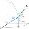Fig. A.1 Computation of unit vector pointing to satellite from azimuth & elevation at station.

• Unit vector pointing into the direction of the projection of the satellite range vector onto the local horizon plane spanned up by ${\displaystyle \overrightarrow{N}}$ and ${\displaystyle \overrightarrow{E}}$ (Fig. A.1, green-red plane and dark blue vector):

$${\displaystyle \overrightarrow{\iota }}={\displaystyle \overrightarrow{N}}\cdot \cos \left(az\right)+{\displaystyle \overrightarrow{E}}\cdot \sin \left(az\right)$$(A.2)

• Unit vector pointing into the direction of the satellite range (Fig. A.1, violet vector):

$${\displaystyle \overrightarrow{I}}={\displaystyle \overrightarrow{\iota }}\cdot \cos \left(el\right)+\frac{{\displaystyle \overrightarrow{R}}}{\left|{\displaystyle \overrightarrow{R}}\right|}\cdot \sin \left(el\right)=\left\{{\displaystyle \overrightarrow{N}}\cdot \cos \left(az\right)+{\displaystyle \overrightarrow{E}}\cdot \sin \left(az\right)\right\}\cdot \cos \left(el\right)+\frac{{\displaystyle \overrightarrow{R}}}{\left|{\displaystyle \overrightarrow{R}}\right|}\cdot \sin \left(el\right)$$(A.3)

Knowing the unit vector pointing from station into satellite range direction, the position vector of the IPP can be computed (Fig. A.2):

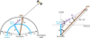Fig. A.2 Computation of the position vector of the IPP.

The magnitude of the IPP position vector is (Fig. A.2, left): 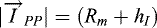$$\left|{{\displaystyle \overrightarrow{I}}}_{PP}\right|=\left(R_m+h_I\right)$$(A.4) where

R_m – mean earth radius, Eq. (10)

h_I – height of ionospheric shell, Eq. (10) Next, sine and cosine values of the auxiliary angles α and β have to be computed (Fig. A.2, right): $$\begin{array}{c}\hfill \begin{array}{ccc}\hfill \cos \alpha =-\cos \zeta =-\frac{{\displaystyle \overrightarrow{R}}}{\left|{\displaystyle \overrightarrow{R}}\right|}\cdot {\displaystyle \overrightarrow{I}}\hfill & \hfill ,\hfill & \hfill \sin \alpha =\sqrt{1-{\cos }^2\alpha }\hfill \end{array}\hfill \\ \hfill \mathrm{}\hfill \\ \hfill \begin{array}{ccc}\hfill \sin \beta =\frac{\left|{\displaystyle \overrightarrow{R}}\right|}{\left(R_m+h_I\right)}\cdot \sin \alpha \hfill & \hfill ,\hfill & \hfill \cos \beta =\sqrt{1-{\sin }^2\beta }\hfill \end{array}\hfill \end{array}$$(A.5)

Applying the cosine rule (e.g. Sigl, 1977): $$c^2=a^2+b^2-2\cdot a\cdot b\cdot \cos \gamma$$(A.6)

And considering: γ = 180⁰ − (α + β) and cos {180⁰ − (α + β)} = − cos(α + β), Eq. (A.6) can be modified to: $$c^2=a^2+b^2+2\cdot a\cdot b\cdot \cos \left(\alpha +\beta \right)$$(A.7)

And with cos(α + β) = cosα ⋅ cosβ − sinα ⋅ sinβ, Eq. (A.7) is modified to: $$c^2=a^2+b^2+2\cdot a\cdot b\cdot \left(\cos \alpha \cdot \cos \beta -\sin \alpha \cdot \sin \beta \right)$$(A.8)

Finally by setting $\mathit{a}=({\mathit{R}}_{\mathit{m}}+{\mathit{h}}_{\mathit{I}}),\mathit{b}=\left|\overrightarrow{\mathit{R}}\right|,\mathit{c}=\mathrm{\Omega }$ and taking the square root of Eq. (A.8), one gets the formulae (A.9) for computing the IPP position vector: $$\begin{array}{ccc}\hfill {{\displaystyle \overrightarrow{I}}}_{PP}={\displaystyle \overrightarrow{R}}+\mathrm{\Omega }\cdot {\displaystyle \overrightarrow{I}}\hfill & \hfill ,\hfill & \hfill \mathrm{\Omega }=\sqrt{{\left(R_m+h_I\right)}^2+{\left|{\displaystyle \overrightarrow{R}}\right|}^2+2\cdot \left(R_m+h_I\right)\cdot \left|{\displaystyle \overrightarrow{R}}\right|\cdot \left(\cos \alpha \cdot \cos \beta -\sin \alpha \cdot \sin \beta \right)}\hfill \end{array}$$(A.9)

References

All Tables

All Figures

	Fig. 1 Time schedule for the daily computer runs at the Navigation Support Office to establish 48h time series of ZWDs and ZTDs, and tropospheric media calibrations.
In the text

	Fig. 2 Ideal case A-matrix structure.
In the text

	Fig. 3 Examples of polynomial fitting in the case of data gaps, marked in red.
In the text

	Fig. 4 Considered vector geometry between DSN station, GNSS satellites and ESA spacecraft/quasar.
In the text

	Fig. 6 Maximal possible geocentric angle ξmax for given mean earth radius RM and ionospheric shell height hI.
In the text

	Fig. 5 Computing weights from the angles enclosed by the IPP position vectors.
In the text

	Fig. 11 (a) Example from Test Case 1; (b) example from Test Case 1 with sTEC simulated by NTCM-GL; (c) example from Test Case 2; (d) example from Test Case 3.
In the text

	Fig. 7 (a) Computing sTECESA/Q only with Eqs. (6)–(9); (b) Measure 1 included; (c) Measure 2 included; (d) Measure 3 included → see Figure 11a.
In the text

	Fig. 8 (a) Example of dry-part polynomials; (b) example of wet-part polynomials.
In the text

	Fig. 9 Overview of Doppler residuals over the full arc used in the GAIA OD; tropospheric corrections based on TRCal.
In the text

	Fig. 10 Comparison of 2-way Doppler residuals with Saastamoinen (top plot) and TRCal (bottom plot) corrections.
In the text

	Fig. 12 Histogram analysis of RMS values.
In the text

	Fig. A.1 Computation of unit vector pointing to satellite from azimuth & elevation at station.
In the text

	Fig. A.2 Computation of the position vector of the IPP.
In the text

References

- Armano M. et al. 2016. Sub-Femto-g Free Fall for Space-Based Gravitational Wave Observatories: LISA Pathfinder Results. Phys Rev Lett 116: 231101. [CrossRef] [Google Scholar]
- Böhm J. 2007. Tropospheric Delay Modelling at Radio Wavelengths for Space Geodetic Techniques. Habilitation Thesis at the Vienna University of Technology, Institute of Geodesy and Geoinformation, Vienna, Austria, Geowissenschaftliche Mitteilungen, Iss. 80. [Google Scholar]
- Budnik F, Morley TA, Mackenzie RA. 2004. ESOĆs System for Interplanetary Orbit Determination: Implementation and Operational Experience, 18th International Symposium on Space Flight Dynamics, Munich (Germany), http://issfd.org/ISSFD_2004/papers/P0118.pdf. [Google Scholar]
- Budnik F, Morley T, Croon M. 2012. Orbit Reconstruction for the GAIA mission. 23rd Symposium on Space Flight Dynamics, Pasadena, California, http://issfd.org/ISSFD_2012/ISSFD23_OD2_5.pdf. [Google Scholar]
- Chao CC. 1973. A New Method to Predict Wet Zenith Range Correction from Surface Measurements. DSN Progress Report, Vol XIV, https://ipnpr.jpl.nasa.gov/progress_report2/XIV/XIVG.PDF. [Google Scholar]
- Coster AJ, Gaposchkin EM, Thornton LE. 1992. Real-Time Ionospheric Monitoring System Using the GPS. Technical Report 954, ESC-TR-91-179, AD-A256 916, Lincoln Laboratory, Massachusetts Institute of Technology, Lexington, Massachusetts, https://pdfs.semanticscholar.org/fd9d/527c1747b72636159ac5ee6fcf1997e01e66.pdf. [Google Scholar]
- Davies K. 1990. Ionospheric Radio. IEE Electromagnetic Wave Series, 31, Peter Peregrinus Ltd., ISBN 0 86341 186 X. [Google Scholar]
- Estefan JA, Sovers OJ. 1994. A Comparative Survey of Current and Proposed Tropospheric Refraction-Delay Models for DSN Radio Metric Data Calibration. JPL Publication 94-24, National Aeronautics and Space Administration, Jet Propulsion Laboratory, California Institute of Technology, Pasadena, CA, USA, https://ntrs.nasa.gov/archive/nasa/casi.ntrs.nasa.gov/19950013586.pdf. [Google Scholar]
- Feltens J. 2008. Vector methods to compute azimuth, elevation, ellipsoidal normal, and the Cartesian (X, Y, Z) to geodetic (φ, λ, h) transformation. J Geod 82: 493–504. [CrossRef] [Google Scholar]
- Jakowski N, Hoque MM, Mayer C. 2011. A new global TEC model for estimating transionospheric radio wave propagation errors. J Geod 85: 965–974, DOI: 10.1007/s00190-011-0455-1. [Google Scholar]
- JPL. 2008. TRK- 2-23 Media Calibration Interface. 820-013, Deep Space Network (DSN), External Interface Specification, JPL D-16765, Revision C (draft), http://dawndata.igpp.ucla.edu/download.jsp?file=documents/Gravity/DATA_SET_DESCRIPTION/TRK-2-23_REVC_L5.PDF. [Google Scholar]
- Kelley MC. 1989. The Earth's Ionosphere, Plasma Physics and Electrodynamics, Academic Press Inc., Harcourt Brace Jovanovich, Publishers, San Diego New York Berkeley Boston London Sydney Tokyo Toronto. [Google Scholar]
- Klobuchar JA. 1975. A First-Order, Worldwide, Ionospheric, Time-Delay Algorithm. Bedford, Mass. United States Air Force, Air Force Systems Command, Air Force Cambridge Research Laboratories, Ionospheric Physics Laboratory. [Google Scholar]
- Komjathy A. 1997. Global Ionospheric Total Electron Content Mapping Using the Global Positioning System. Ph.D. dissertation, Department of Geodesy and Geomatics Engineering Technical Report No. 188, University of New Brunswick, Fredericton, New Brunswick, Canada. [Google Scholar]
- Lagler K, Schindelegger M, Böhm J, Krásná H, Nilsson T. 2013. GPT2: Empirical slant delay model for radio space geodetic techniques. Geophys Res Lett 40: 1069–1073, DOI:10.1002/grl.50288. [CrossRef] [Google Scholar]
- Mannucci AJ, Wilson BD, Yuan DN, Ho CH, Lindquister UJ, Runge TF. 1998. A global mapping technique for GPS-derived ionospheric total electron content measurements. Radio Sci 33: 565–582. [Google Scholar]
- Moyer TD. 1971. Mathematical formulation of the Double Precision Orbit Determination Program (DPODP), NASA-JPL report JPL-TR-32-1527, Jet Propulsion Laboratory, https://ntrs.nasa.gov/archive/nasa/casi.ntrs.nasa.gov/19710017134.pdf. [Google Scholar]
- Moyer TD. 2000. Formulation for Observed and Computed Values of Deep Space Network Data Types for Navigation, Deep Space Communications and Navigation Systems, Jet Propulsion Laboratory, Publication 00-7, https://descanso.jpl.nasa.gov/monograph/series2/Descanso2_all.pdf. [Google Scholar]
- Niell AE. 1996. Global mapping functions for the atmosphere delay at radio wavelengths. J Geophys Res 101: 3227–3246. [NASA ADS] [CrossRef] [Google Scholar]
- Niell AE. 2000. Improved atmospheric mapping functions for VLBI and GPS. Earth Planets Space 52: 699–702. [CrossRef] [Google Scholar]
- Ratcliffe JA. 1972. An introduction to the ionosphere and magnetosphere, Cambridge University Press, Great Britain. [Google Scholar]
- Saastamoinen JJ. 1973. Contributions to the theory of atmospheric refraction. Bulletin Géodesique 107: 13–34. [CrossRef] [Google Scholar]
- Schaer S. 1999. Mapping and predicting the Earth's Ionosphere using the Global Positioning System, PhD Thesis, AIUB, University of Berne, Switzerland. [Google Scholar]
- Schaer S, Gurtner W, Feltens J. 1998. IONEX: The IONosphere Map Exchange Format Version 1. In: Proceedings of the IGS Analysis Centres Workshop. Darmstadt, Germany. [Google Scholar]
- Seeber G. 2003. Satellite Geodesy, 2nd edition, Walter de Gruyter, Berlin, New York. [CrossRef] [Google Scholar]
- Sigl R. 1977. Ebene und Sphärische Trigonometrie, Hermann Wichmann Verlag, Karlsruhe. [Google Scholar]
- Steigenberger P, Böhm J, Tesmer V. 2009. Comparison of GMF/GPT with VMF1/ECMWF and implications for atmospheric loading. J Geod 83: 943–951, DOI: 10.1007/s00190-009-0311-8. [CrossRef] [Google Scholar]
Cite this article as: Feltens J, Bellei G, Springer T, Kints MV, Zandbergen R, Budnik F, Schönemann E. 2018. Tropospheric and ionospheric media calibrations based on global navigation satellite system observation data. J. Space Weather Space Clim. 8: A30
All Tables
RMS summary on tropospheric polynomial fitting, 12 April 2016, 12:00–14 April 2016, 12:00.
Mean, standard deviation, minimal and maximal RMS values of the three test cases.