| Issue |
J. Space Weather Space Clim.
Volume 14, 2024
|
|
|---|---|---|
| Article Number | 20 | |
| Number of page(s) | 8 | |
| DOI | https://doi.org/10.1051/swsc/2024020 | |
| Published online | 01 August 2024 | |
Technical Article
Updated model of cosmic-ray-induced ionization in the atmosphere (CRAC:CRII_v3): Improved yield function and lookup tables
1
Space Physics and Astronomy Research Unit and Sodankylä Geophysical Observatory, University of Oulu, Linanmaa 90014, Finland
2
A.F. Ioffe Physical–Technical Institute, Politechnicheskaya 26, 194021 St. Petersburg, Russia
* Corresponding author: This email address is being protected from spambots. You need JavaScript enabled to view it.
Received:
1
March
2024
Accepted:
29
May
2024
Abstract
Cosmic rays, including galactic cosmic rays and solar energetic particles, form the main source of ionization of the low and middle atmosphere, which is important for various chemical and physical effects in the atmosphere. Realistic models able to compute the cosmic-ray-induced ionization (CRII) are used as inputs for chemistry-climate models. One of the most commonly used atmospheric ionization models is CRAC:CRII (Cosmic-Ray Atmospheric Cascade: application to CRII) initially developed in 2004–2006 (version 1) and significantly improved in 2010–2011 (version 2). Here, a new updated version 3 of the CRAC:CRII model is presented which offers a higher accuracy for the middle-upper atmosphere and lower-energy cosmic rays. This is particularly important for studies of the atmospheric effects of solar particle storms. Detailed lookup tables of the ionization yield function are provided for the primary cosmic ray protons and α-particles (the latter representing also heavier cosmic-ray species) along with a practical recipe for their numerical use.
Key words: Cosmic rays / Atmosphere / Ionization / Numerical models
© I.G. Usoskin et al., Published by EDP Sciences 2024
 This is an Open Access article distributed under the terms of the Creative Commons Attribution License (https://creativecommons.org/licenses/by/4.0), which permits unrestricted use, distribution, and reproduction in any medium, provided the original work is properly cited.
1 Introduction
The Earth’s atmosphere is constantly bombarded by high-energy particles originating from outer space that are called cosmic rays (CRs). The most important are Galactic CRs (GCRs), which originate from the Galaxy – they have omnipresent and nearly isotropic flux near Earth with a slight variability at different timescales. The energy of GCRs is typically in the range of several GeV/nucleon and can reach up to 1020 eV. GCRs near Earth mostly consist of protons (about 90%), helium (about 9%), and 1% of heavier element nuclei, produced mostly by supernovae in the Galaxy (see, e.g., Gaisser et al., 2016, and references therein). High-energy particles can be also accelerated near the Sun in solar eruptive events such as flares or coronal mass ejections – they are called solar energetic particles (SEPs) and have sporadic occurrence and very strong variability (e.g., Desai and Giacalone, 2016). The energy of SEPs is typically below 100 MeV but in rare cases of very energetic events, called ground-level enhancements (GLEs), it can reach several GeV. The third type of CRs, the anomalous cosmic rays originating from interstellar neutral atoms, is not considered here as having too low energy and fluxes to affect the atmosphere.
Because of the geomagnetic field and its shielding effect, the flux of GCRs impinging on Earth is not uniform being higher in polar regions and lowest in the equatorial region. SEPs can enter the Earth’s atmosphere in (sub)polar regions with only very rare events being detectable at mid and low latitudes.
When entering the Earth’s atmosphere, energetic particles interact with matter losing energy for ionization of the ambient air (e.g., Bazilevskaya et al., 2008). If the particle’s energy is sufficiently high, inelastic nuclear collisions become also important leading to the formation of a complicated hadron-electromagnetic-muon cascade of secondary particles, known also as extensive air shower (for details see, e.g., Dorman, 2004; Grieder, 2011; Gaisser et al., 2016). CRs form the main source of atmospheric ionization, called cosmic-ray-induced ionization (CRII) below ≈100 km height (e.g., Vainio et al., 2009) with the maximum of ion production lying at the altitude of about 12–15 km in the atmosphere (Regener and Pfotzer, 1935). Other effects, such as solar UV and X-rays as well as magnetospheric particles, can drive ionization at higher altitudes (e.g., Mironova et al., 2015). Besides, natural radionuclides can contribute to atmospheric ionization in the near-ground layer (e.g., Eisenbud and Gesell, 1997). CRII plays a crucial role in the physical and chemical atmospheric processes (e.g. Crutzen et al., 1975; Randall et al., 2007; Calisto et al., 2011; Semeniuk et al., 2011; Rozanov et al., 2012; Sinnhuber et al., 2012; Jackman et al., 2016; Golubenko et al., 2020).
While the physics of atmospheric ionization is well understood (e.g., Mironova et al., 2015), the exact modelling of CRII remains slightly uncertain, particularly in the upper-middle atmosphere. The ion production in the upper atmosphere can be calculated using analytical (parameterization) and/or semi-empirical models (e.g., Vitt and Jackman, 1996; Turunen et al., 2009; McGranaghan et al., 2015). Such analytical models have limited applicability to only the upper polar atmospheric region and lower-energy particles (below 100 MeV) because they neglect inelastic scattering and the development of the atmospheric cascade. Their applicability at heights below 40 km and outside the polar cusp region is not validated (Desorgher et al., 2009; Velinov et al., 2013; Mironova et al., 2015). CRII in the low and middle atmosphere is well-modelled by full Monte Carlo models which simulate the atmospheric cascade using the modern knowledge of nuclear reactions. The most widely used full Monte-Carlo models are PLANETOCOSMIC (Desorgher et al., 2005, 2009) and CRAC:CRII (Cosmic-Ray Atmospheric Casacde: application to CRII – Usoskin et al., 2004; Usoskin and Kovaltsov, 2006; Usoskin et al., 2010). The latter is a reference model, e.g., for the CMIP (Climate Model Intercomparison Project – see Matthes et al., 2017; Jungclaus et al., 2017; Funke et al., 2024) phases 6 and 7. Full Monte-Carlo models precisely, within the 10% accuracy, compute CRII for the low and middle atmosphere with the residual atmospheric depth >10 g/cm2 (e.g., Usoskin et al., 2009) but may be less certain in the upper atmosphere, where the cascade is not yet induced, and the Monte Carlo approach is not optimal. Thus, a combination of the Monte Carlo models for the lower and middle atmosphere and the analytical approach for the upper polar atmosphere is required for consistent modelling of ionization of the whole atmosphere. Such work was done firstly by Usoskin et al. (2010), and here we extend and upgrade that work by updating the computations and providing detailed lookup tables so that a user can compute cosmic-ray-induced ionization at any location and initial conditions.
2 Monte Carlo model
Since energetic particles initiate a complicated cascade in the atmosphere, it is important to model it in a realistic way. At each hadronic interaction, about one-third of primary CR particle energy is transferred to the electromagnetic component of the developing shower, that is electrons, positrons and γ-quanta. Secondary hadrons experience subsequent interactions, leading to most of the primary particle’s energy being dissipated by ionization energy losses of the electromagnetic component (see, e.g., chapter 16 in Gaisser et al., 2016). The most suitable way to model this process is a Monte Carlo approach which takes into account all known processes (Desorgher et al., 2005; Usoskin and Kovaltsov, 2006). Such models are based on a full Monte Carlo simulation of CR particle propagation and interaction in the atmosphere, employing the recent achievements of particle physics and the corresponding hadron generation simulators. The main advantage of Monte Carlo transport codes is that they consider realistically all the physical processes, including secondary and subsequent-generation particle production and propagation as well as energy losses, which contribute eventually to the ionization of air, specifically at lower and middle altitudes (e.g., Bazilevskaya et al., 2008; Usoskin et al., 2009; Mironova et al., 2015, and references therein).
There are different Monte-Carlo-based models of CRII, but some of them have limitations on the energy range or particle species (e.g. Wissing and Kallenrode, 2009; Mishev and Velinov, 2010). Two most useful models are CRAC:CRII (versions 1 and 2 – Usoskin and Kovaltsov, 2006; Usoskin et al., 2010, respectively) based on COSRIKA simulation tool (COsmic Ray SImulations for KAscade – Heck et al., 1998) and PLANETOCOSMICS (Desorgher et al., 2005) based on GEANT4 tool (GEometry ANd Tracking – Agostinelli et al., 2003). It is important that at the present level of knowledge, different Monte Carlo tools would produce similar averaged results (Usoskin et al., 2009) if based on the same atmospheric model and physics list, considering the intrinsic shower fluctuations (see discussion in Engel et al., 2011; Pierog, 2017). Thus, an inter-model comparison is not crucial.
We note that presently only the CRAC:CRII model provides look-up tables in the form of yield functions making fast yet accurate CRII computations possible for any given location and energetic-particle spectrum (see Usoskin and Kovaltsov, 2006, also available at https://cosmicrays.oulu.fi/CRII/CRII.html).
Herewith we update and extend the CRAC:CRII model (Usoskin and Kovaltsov, 2006; Usoskin et al., 2010), upgrading it to version 3. First, we performed the high-statistic Monte Carlo simulations of the atmospheric cascade and the deposited energy for two types of the primary CR particles, protons and α-particles, the latter effectively representing also heavier species (Koldobskiy et al., 2019), assuming their isotropic flux on the top of the atmosphere. The simulations were performed using a Fortran-based CORSIKA code (v.6.617 – Heck et al., 1998) extended with FLUKA (v.2006.3b – Fassò et al., 2001) in the low-energy range. We applied a realistic spherical geometry of the atmosphere which is important for the isotropic flux, the atmospheric parameters were considered according to the NRLMSISE-00 model (Picone et al., 2002). The statistic of the simulated primary particles was improved to keep the statistical uncertainty generally below 1% – the number of simulated showers varied between 103 and 107 for each energy point depending on the primary particle’s energy.
We used an improved grid over energy – 20 logarithmically spaced energy values per order of magnitude between 10 MeV and 1000 GeV; and over atmospheric depth – 0.01 g/cm2 steps between 0 and 0.1 g/cm2, 0.1 g/cm2 steps between 0.1 and 1 g/cm2, 1 g/cm2 between 1 and 10 g/cm2, and 5 g/cm2 for the depths greater than 10 g/cm2. This grid is much denser than that used in CRAC:CRII versions 1 and 2 (two points over an order of magnitude in energy and 50 g/cm2 over the atmospheric depth), which allows us to improve the accuracy of the computations. The energy deposition was converted into the ion-pair production assuming 35 eV per ion pair (Porter et al., 1976). The obtained grid values of the CRII were locally smoothed in two dimensions (energy and atmospheric depth).
However, Monte Carlo models can be imprecise in the upper atmosphere, at the atmospheric depth <10 g/cm2, where the cascade is not developed and CRII is dominated by the direct ionization by the primary CR particle as illustrated in Figure 1. This process is not always accurately considered in the Monte Carlo simulation tools and may lead to imprecise results in the upper atmosphere (e.g., Mishev and Velinov, 2010, 2014). To overcome this problem we combined the Monte Carlo simulation with the analytical calculation of the direct ionization of the ambient air by the primary particle before its first inelastic nuclear interaction.
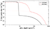 |
Figure 1 Dependence of the ionization yield function Y(h) (see Eq. (9)) on the atmospheric depth h for primary protons with different kinetic energies, as indicated in the legend. Two components can be observed, viz. direct ionization by the primary particles which dominate the upper atmosphere, and the ionization by secondaries of the atmospheric cascade which dominates in the lower atmosphere. An extension of the cascade-induced ionization to the upper atmosphere is depicted by thin dashed curves. |
3 Analytical solution for the upper atmosphere
For the uppermost layer of the atmosphere, with a depth <10 g/cm2, ionization can be calculated analytically without employing a full Monte Carlo model.
Let us consider a locally flat atmosphere as illustrated in Figure 2. The vertical dimension is the atmospheric depth (or thickness) h in units of g/cm2 where h = 0 corresponds to the top of the atmosphere. An energetic particle (proton) with energy E enters the atmosphere at the zenith angle θ (henceforth we denote μ = cos(θ)). If other energy losses but ionization of the ambient air can be neglected as well as the scattering of the particle, the proton’s energy ε(h) at the depth h can be defined as
 (1)
(1)
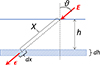 |
Figure 2 Scheme of the upper atmosphere used for the analytical solution. The upper horizontal blue line denotes the top of the atmosphere, where a particle with energy E enters at the zenith angle θ. Energy deposition at the atmospheric depth h is considered in a thin layer of dh thickness where the particle has energy ε. The pathlength of the particle in the air between the top of the atmosphere and the depth h is denoted as X = h/cos(θ). |
where X = h/μ is the proton’s pathlength to the depth h, R(ε) is the full pathlength of the proton with energy ε before full breaking by ionization loss, defined as
 (2)
(2)
where  is the ionizing loss of a particle with energy E′ in air (Berger et al., 2017). The maximum pathlength of the particle with the initial energy E is denoted as R* = R(E). Let us denote the stopping power (energy loss per unit thickness) of the particle in the air as
 (3)
(3)
where energy ε is defined from equation (1). Equation (1) is obtained for one primary particle impinging on the atmosphere with the zenith angle θ. Let us denote the distribution of the particle intensity on the cosine μ of the zenith angle on the top of the atmosphere as dI/dμ, then one can find the energy deposited (per unit depth) at the atmospheric depth h as
 (4)
(4)
where μmin = h/R(E) is the minimum cosine of the zenith angle so that the particle with initial energy E can still reach the depth h before losing all its energy.
For the isotropic angular distribution (normalized per one particle on the top of the atmosphere) of primary particles, where  , equation (4) becomes
 (5)
(5)
Since for any given R* and h, the cosine μ can be expressed via R as
 (6)
(6)
and equation (4) becomes
 (7)
(7)
The stopping-power range in dry air is known (e.g., Berger et al., 2017) and can be used to compute the deposited energy (per unit atmospheric depth) G for any given E and h.
In addition to these ionization energy losses, inelastic-collision losses of particles need to be considered (see, e.g., Section 3 in Usoskin et al., 2010). This process is usually neglected in the upper atmosphere but naturally taken care of by the Monte Carlo models in the low and middle atmosphere.
Accordingly, here we performed a smooth junction of the full Monte Carlo modelling performed in most of the atmosphere and direct analytical solutions for the upper atmospheric level.
4 Yield function and lookup tables
The results of the modelling are presented in the form of tabulated ionization yield functions which allow a user to compute CRII at any given location straightforwardly without the full computationally heavy modelling of the atmospheric cascade. Here, we provide a brief description of the approach, while more details can be found in our earlier works (Usoskin and Kovaltsov, 2006; Usoskin et al., 2010).
From the Monte Carlo simulations, we obtained the mean number of ion pairs per g/cm2 produced by a single primary particle with energy E in a thin atmospheric layer at the atmospheric depth h, called the ion production function S, as
 (8)
(8)
where G(E,h) is the mean energy deposition per unit atmospheric thickness of all the primary and secondary particles at the atmospheric depth h, and Ei = 35 eV is the average energy for the production of an ion pair in air (Porter et al., 1976). The production function was computed separately for protons, Fp, and α-particles, Fα. Usually, the yield-function Y (ion pairs sr cm2 g−1) is considered which quantifies the ion production not for a single primary particle but for a unit intensity of the primary particles with the fixed energy E on the top of the atmosphere. For the isotropic flux of primary particles, the two quantities are related as
 (9)
(9)
where π is the geometrical normalization factor. The tabulated values for both protons and α-particles are given in the Supplementary materials to this paper. The values of Y for α-particle are provided per nucleon of the primary α-particle. The ionization rate in the air at the depth h is then defined as an integral of the product of the yield function Yn(h,E) of primary particles of type n with the energy spectrum Jn(E)
 (10)
(10)
where the summation is over the types n of primary CR particles (protons, α-particles) characterized by the charge and atomic numbers Zn and An, respectively, and integration is over energy above the energy corresponding to the local geomagnetic rigidity cutoff Pc (Cooke et al., 1991) as
 (11)
(11)
where Er is the proton’s rest mass.
This approach works for all primary particles – whether lower-energy solar energetic particles (SEPs) with a soft spectrum or more energetic galactic cosmic rays (GCRs) with a harder spectrum. Since SEPs consist of mostly protons, the sum in equation (10) disappears and only the yield function for protons is considered. GCRs have richer compositions, but heavier (Z > 2) species are similar to α-particles in the sense of the Z/A ≈ 2 ratio implying that they experience similar heliospheric and magnetospheric modulation. Accordingly, it is customary to account for Z > 2 nuclei by scaling the flux α-particle (Koldobskiy et al., 2019).
Here we provide the pre-computed and verified lookup tables of CRII as a function of the atmospheric depth h and energy E. The lookup tables provide the ionization yield functions Y(h, E) with a sufficiently dense grid. This is illustrated in Figures 3 and 4. Figure 3 depicts the tabulated CRII as a function of the primary proton’s energy for two layers of h = 1 and 3 g/cm2 (about 50 and 40 km for the standard atmosphere, respectively), for the results of CRAC:CRII_v3 presented here (red curve) and the previous version 2. As seen, the new denser grid covers the lower-energy range with much higher accuracy, specifically in the energy range of several hundred MeV which is important for SEPs. Accordingly, the new results improve the accuracy of the CRII computation due to SEPs in the upper atmosphere. Figure 4 depicts the tabulated CRII as a function of the atmospheric depth for two values of the primary proton’s energy of 0.1 GeV and 0.5 GeV. As seen, the altitude profile of CRII was distorted in model version 2 for low-energy particles in the middle atmosphere h < 25 g/cm2 (above ≈25 km), while the results are consistent between the versions for higher energies and deeper atmospheric layers.
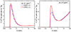 |
Figure 3 Comparison between the ionization yield functions Y in the CRAC:CRII versions 2 (blue) and 3 (red) as functions of the primary particles energy for two layers in the upper atmosphere of 1 g/cm2 (panel a) and 3 g/cm2 (panel b). |
 |
Figure 4 Comparison between the ionization yield functions Y in the CRAC:CRII versions 2 (blue) and 3 (red) as functions of the atmospheric depth h for two values of the particle’s energy of 0.1 GeV (panel a) and 0.5 GeV (panel b). |
5 Recipe for the use of lookup tables
The provided grid is sufficiently dense so that the values between the grid points can be interpolated using a power-law interpolation (linear in the double logarithmic space) as follows. A simple linear interpolation between the grid points may lead to essential inaccuracy.
Let us estimate the value of a function Y(h,E), where the values of h and E lie between the grid points hi − hi+1 and Ej − Ej+1, respectively. Let y, η and e be logS, logh and logE, respectively. Then
 (12)
(12)
where
 (13)
(13)
Then,
 (14)
(14)
The ion production rate Q(h) for any air depth h can be calculated using equation (10) where integration is replaced by summation over the grid points in energy.
 (15)
(15)
where Fj,n = J(Ej)⋅Yn(h, Ej) is the value of the integrand at the energy gridpoint j for the particle of type n. Because of the very steep integrand function, the local power-law approximation of the integrand between the grid points j and j+1 is recommended:
 (16)
(16)
6 Example of CRII computations
As an example of the use of the lookup tables, we present in Figure 5 the computed atmospheric ionization by GCRs as a function of the geomagnetic latitude and atmospheric depth for the conditions of 2015. The spectrum of GCR was modelled using the force-field parameterization with the value of the modulation potential ϕ = 645 MV corresponding to the year 2015 (Usoskin et al., 2017). The geomagnetic shielding was calculated using the standard vertical geomagnetic rigidity cutoff methodology (see Nevalainen et al., 2013, for details). The geomagnetic field was considered as the International Geomagnetic Reference Field (IGRF – Thébault et al., 2015) for the epoch 2015. As one can see from Figure 5, the maximum of the ion production occurs at the atmospheric level of 50–100 g/cm2 (10–20 km) in the polar atmosphere. This corresponds to the Regener-Pfotzer maximum where the nucleonic cascade effectively starts. At deeper layers, the intensity of the cascade decreases leading to lower ionization rates. The relatively high ionization rate in the upper layers of the polar atmosphere (h < 50 g/cm2) is caused by the high flux of lower-energy cosmic rays which can directly ionize the air. Such low-energy particles are absent at lower latitudes because of the geomagnetic shielding leading to low CRII in the upper atmosphere. The ionization rate decreases towards the equator due to the geomagnetic shielding but also has a higher location at the Regener-Pfotzer maximum. Thus, the present model reproduces all the main characteristic patterns of the CRII (e.g., Bazilevskaya et al., 2008; Mironova et al., 2015).
 |
Figure 5 Cosmic-ray-induced ionization (CRII) as a function of the geomagnetic latitude λgeom and common logarithm of the atmospheric depth h (in g/cm2) for the geomagnetic field and solar modulation corresponding to the year 2015. |
7 Summary
Here we present an updated version (v.3) of the CRAC:CRII model of cosmic-ray-induced ionization of the atmosphere, which is one of the most commonly used ones in related atmospheric research. The updated version includes the core Monte-Carlo-based cascade simulations (similar to that of version 2) for the low and middle atmosphere extended by the results of an analytical integration, using the stopping-power approach, of the direct ionization in the upper atmosphere. The lookup tables of the ionization yield function are provided for protons and α-particles (the latter effectively representing heavier cosmic-ray species) in the energy range from 1 MeV to 1000 GeV and the atmospheric-depth range from the ground (1033 g/cm2) to the top of the atmosphere. The grid at which the lookup tables are presented is much denser than in the previous versions: 20 logarithmically spaced points per decade in energy, 10 equispaced points per decade in the atmospheric depth h ≤ 10 g/cm2, and 5 g/cm2 resolution for h > 10 g/cm2. A detailed recipe for the numerical use of lookup tables is provided so that it is straightforward to compute the CRII rate at any location and time (providing the cosmic-ray spectrum and geomagnetic shielding are known independently) and thus to implement the results of CRAC:CRII_v.3 model to any kind of atmospheric model. The CRAC:CRII_v.3 model is suited to compute the atmospheric ionization induced by galactic cosmic rays, solar energetic particles or any other energetic protons or heavier species with a nearly isotropic spatial distribution.
Acknowledgments
The work was partly done in the framework of project No.354280 of the Research Council of Finland. The editor thanks Fan Lei and an anonymous reviewer for their assistance in evaluating this paper.
Data availability statement
The pre-computed tables of the ionization yield functions for protons and α-particles are available as the Supplementary materials to this paper and also deposited at https://cosmicrays.oulu.fi/CRII/CRII.html.
Supplementary material
Look-up table for alpha-particle yield function.
Look-up table for proton yield function.
Access Supplementary MaterialReferences
- Agostinelli S, Allison J, Amako K, Apostolakis J, Araujo H, et al. 2003. Geant4-a simulation toolkit. Nucl Instr Meth Phys Res A 506: 250–303. https://doi.org/10.1016/S0168-9002(03)01368-8. [CrossRef] [Google Scholar]
- Bazilevskaya GA, Usoskin IG, Flückiger EO, Harrison RG, Desorgher L, et al. 2008. Cosmic ray induced ion production in the atmosphere. Space Sci Rev 137: 149–173. https://doi.org/10.1007/s11214-008-9339-y. [CrossRef] [Google Scholar]
- Berger M, Coursey J, Zucker M, Chang J. 2017. NIST stopping-power and range tables for electrons, protons, and helium ions – SRD 124. Tech. Rep., NIST. https://doi.org/10.18434/T4NC7P. [Google Scholar]
- Calisto M, Usoskin I, Rozanov E, Peter T. 2011. Influence of galactic cosmic rays on atmospheric composition and dynamics. Atmos Chem Phys 11: 4547–4556. https://doi.org/10.5194/acp-11-4547-2011. [CrossRef] [Google Scholar]
- Cooke D, Humble J, Shea M, Smart D, Lund N, Rasmussen I, Byrnak B, Goret P, Petrou N. 1991. On cosmic-ray cut-off terminology. Nuovo Cimento C 14: 213–234. https://doi.org/10.1007/BF02509357. [CrossRef] [Google Scholar]
- Crutzen PJ, Isaksen ISA, Reid GC. 1975. Solar proton events: stratospheric sources of nitric oxide. Science 189(4201): 457–459. https://doi.org/10.1126/science.189.4201.457. [CrossRef] [Google Scholar]
- Desai M, Giacalone J. 2016. Large gradual solar energetic particle events. Liv Rev Solar Phys 13: 3. https://doi.org/10.1007/s41116-016-0002-5. [CrossRef] [Google Scholar]
- Desorgher L, Flückiger EO, Gurtner M, Moser MR, Bütikofer R. 2005. Atmocosmics: a Geant 4 Code for computing the interaction of cosmic rays with the Earth’s atmosphere. Int J Modern Phys A 20: 6802–6804. https://doi.org/10.1142/S0217751X05030132. [CrossRef] [Google Scholar]
- Desorgher L, Kudela K, Flückiger E, Buetikofer R, Storini M, Kalegaev V. 2009. Comparison of Earth’s magnetospheric magnetic field models in the context of cosmic ray physics. Acta Geophys 57(1): 75. https://doi.org/10.2478/s11600-008-0065-3. [CrossRef] [Google Scholar]
- Dorman L. 2004. Cosmic rays in the Earth’s atmosphere and underground. Kluwer Academic Publishers, Dordrecht. [CrossRef] [Google Scholar]
- Eisenbud M, Gesell T. 1997. Environmental radioactivity from natural, industrial and military sources. Academic Press, Cambridge, MA. ISBN 9780122351549. [Google Scholar]
- Engel R, Heck D, Pierog T. 2011. Extensive air showers and hadronic interactions at high energies. Annu Rev Nucl Part Sci 61: 467–489. https://doi.org/10.1146/annurev.nucl.012809.104544. [CrossRef] [Google Scholar]
- Fassò A, Ferrari A, Ranft J, Sala P. 2001. FLUKA: status and prospective of hadronic applications. In A. K. et al., ed., Proc. Monte Carlo 2000 Conf., 955–960. Springer, Berlin. [Google Scholar]
- Funke B, Dudok de Wit T, Ermolli I, Haberreiter M, Kinnison D, Marsh D, Nesse H, Seppälä A, Sinnhuber M, Usoskin I. 2024. Towards the definition of a solar forcing dataset for CMIP7. Geosci Model Dev 17(3): 1217–1227. https://doi.org/10.5194/gmd-17-1217-2024. [CrossRef] [Google Scholar]
- Gaisser T, Engel R, Resconi E. 2016. Cosmic rays and particle physics. Cambridge University Press, Cambridge, UK. ISBN 9781139192194. [CrossRef] [Google Scholar]
- Golubenko K, Rozanov E, Mironova I, Karagodin A, Usoskin I. 2020. Natural sources of ionization and their impact on atmospheric electricity. Geophys Res Lett 47(12): e88619. https://doi.org/10.1029/2020GL088619. [CrossRef] [Google Scholar]
- Grieder P. 2011. Extensive air showers: high energy phenomena and astrophysical aspects. Space Science Library, Springer, NY. ISBN 978-3540769408. [Google Scholar]
- Heck D, Knapp J, Capdevielle J, Schatz G, Thouw T. 1998. CORSIKA: a Monte Carlo Code to simulate extensive air showers. In: FZKA 6019. Forschungszentrum, Karlsruhe. [Google Scholar]
- Jackman CH, Marsh DR, Kinnison DE, Mertens CJ, Fleming E. 2016. Atmospheric changes caused by galactic cosmic rays over the period 1960–2010. Atmos Chem Phys 16(9): 5853–5866. https://doi.org/10.5194/acp-16-5853-2016. [CrossRef] [Google Scholar]
- Jungclaus JH, Bard E, Baroni M, Braconnot P, Cao J, et al. 2017. The PMIP4 contribution to CMIP6 – Part 3: The last millennium, scientific objective, and experimental design for the PMIP4 past1000 simulations. Geosci Model Dev 10(11): 4005–4033. https://doi.org/10.5194/gmd-10-4005-2017. [CrossRef] [Google Scholar]
- Koldobskiy SA, Bindi V, Corti C, Kovaltsov G, Usoskin I. 2019. Validation of the neutron monitor yield function using data from AMS-02 experiment 2011–2017. J Geophys Res (Space Phys) 124: 2367–2379. https://doi.org/10.1029/2018JA026340. [CrossRef] [Google Scholar]
- Matthes K, Funke B, Andersson ME, Barnard L, Beer J, et al. 2017. Solar forcing for CMIP6 (v3.2). Geosci Model Dev 10: 2247–2302. https://doi.org/10.5194/gmd-10-2247-2017. [CrossRef] [Google Scholar]
- McGranaghan R, Knipp D, Solomon S, Fang X. 2015. A fast, parameterized model of upper atmospheric ionization rates, chemistry, and conductivity. J Geophys Res (Space Phys) 120(6): 4936–4949. https://doi.org/10.1002/2015JA021146. [CrossRef] [Google Scholar]
- Mironova IA, Aplin KL, Arnold F, Bazilevskaya GA, Harrison RG, Krivolutsky AA, Nicoll KA, Rozanov EV, Turunen E, Usoskin IG. 2015. Energetic particle influence on the Earth’s atmosphere. Space Sci Rev 194: 1–96. https://doi.org/10.1007/s11214-015-0185-4. [CrossRef] [Google Scholar]
- Mishev AL, Velinov P. 2010. The effect of model assumptions on computations of cosmic ray induced ionization in the atmosphere. J Atmos Solar-Terr Phys 72(5–6): 476–481. https://doi.org/10.1016/j.jastp.2010.01.004. [CrossRef] [Google Scholar]
- Mishev AL, Velinov PIY. 2014. Influence of hadron and atmospheric models on computation of cosmic ray ionization in the atmosphere-Extension to heavy nuclei. J Atmos Solar-Terr Phys 120: 111–120. https://doi.org/10.1016/j.jastp.2014.09.007. [CrossRef] [Google Scholar]
- Nevalainen J, Usoskin IG, Mishev A. 2013. Eccentric dipole approximation of the geomagnetic field: application to cosmic ray computations. Adv Space Res 52: 22–29. https://doi.org/10.1016/j.asr.2013.02.020. [CrossRef] [Google Scholar]
- Picone JM, Hedin AE, Drob DP, Aikin AC. 2002. NRLMSISE-00 empirical model of the atmosphere: Statistical comparisons and scientific issues. J Geophys Res 107: 1468. https://doi.org/10.1029/2002JA009430. [Google Scholar]
- Pierog T. 2017. Open issues in hadronic interactions for air showers. EPJ Web Conf 145: 18002. https://doi.org/10.1051/epjconf/201614518002. [CrossRef] [EDP Sciences] [Google Scholar]
- Porter HS, Jackman CH, Green AES. 1976. Efficiencies for production of atomic nitrogen and oxygen by relativistic proton impact in air. J Chem Phys 65: 154–167. https://doi.org/10.1063/1.432812. [CrossRef] [Google Scholar]
- Randall CE, Harvey VL, Singleton CS, Bailey SM, Bernath PF, Codrescu M, Nakajima H, Russell JM. 2007. Energetic particle precipitation effects on the Southern Hemisphere stratosphere in 1992–2005. J Geophys Res (Atmos) 112(D8): D08308. https://doi.org/10.1029/2006JD007696. [CrossRef] [Google Scholar]
- Regener E, Pfotzer G. 1935. Vertical intensity of cosmic rays by threefold coincidences in the stratosphere. Nature 136: 718–719. https://doi.org/10.1038/136718a0. [CrossRef] [Google Scholar]
- Rozanov E, Calisto M, Egorova T, Peter T, Schmutz W. 2012. Influence of the precipitating energetic particles on atmospheric chemistry and climate. Surv Geophys 33: 483. https://doi.org/10.1007/s10712-012-9192-0. [CrossRef] [Google Scholar]
- Semeniuk K, Fomichev VI, McConnell JC, Fu C, Melo SML, Usoskin IG. 2011. Middle atmosphere response to the solar cycle in irradiance and ionizing particle precipitation. Atmos Chem Phys 11: 5045–5077. https://doi.org/10.5194/acp-11-5045-2011. [CrossRef] [Google Scholar]
- Sinnhuber M, Nieder H, Wieters N. 2012. Energetic particle precipitation and the chemistry of the mesosphere/lower thermosphere. Surv Geophys 33(6): 1281–1334. https://doi.org/10.1007/s10712-012-9201-3. [CrossRef] [Google Scholar]
- Thébault E, Finlay CC, Beggan CD, Alken P, Aubert J, et al. 2015. International geomagnetic reference field: the 12th generation. Earth Planets Space 67: 79. https://doi.org/10.1186/s40623-015-0228-9. [CrossRef] [Google Scholar]
- Turunen E, Verronen P, Seppälä A, Rodger C, Clilverd M, Tamminen J, Enell C, Ulich T. 2009. Impact of different energies of precipitating particles on NOx generation in the middle and upper atmosphere during geomagnetic storms. J Atmos Solar-Terr Phys 71(10–11): 1176–1189. https://doi.org/10.1016/j.jastp.2008.07.005. [CrossRef] [Google Scholar]
- Usoskin IG, Desorgher L, Velinov P, Storini M, Flückiger EO, Bütikofer R, Kovaltsov GA. 2009. Ionization of the earth’s atmosphere by solar and galactic cosmic rays. Acta Geophys 57: 88–101. https://doi.org/10.2478/s11600-008-0019-9. [CrossRef] [Google Scholar]
- Usoskin IG, Gil A, Kovaltsov GA, Mishev AL, Mikhailov VV. 2017. Heliospheric modulation of cosmic rays during the neutron monitor era: calibration using PAMELA data for 2006–2010. J Geophys Res (Space Phys) 122: 3875–3887. https://doi.org/10.1002/2016JA023819. [CrossRef] [Google Scholar]
- Usoskin IG, Gladysheva OG, Kovaltsov GA. 2004. Cosmic ray-induced ionization in the atmosphere: spatial and temporal changes. J Atmos Solar-Terr Phys 66: 1791–1796. https://doi.org/10.1016/j.jastp.2004.07.037. [CrossRef] [Google Scholar]
- Usoskin IG, Kovaltsov GA. 2006. Cosmic ray induced ionization in the atmosphere: full modeling and practical applications. J Geophys Res 111: D21206. https://doi.org/10.1029/2006JD007150. [CrossRef] [Google Scholar]
- Usoskin IG, Kovaltsov GA, Mironova IA. 2010. Cosmic ray induced ionization model CRAC:CRII: an extension to the upper atmosphere. J Geophys Res 115(D14): D10302. https://doi.org/10.1029/2009JD013142. [CrossRef] [Google Scholar]
- Vainio R, Desorgher L, Heynderickx D, Storini M, Flückiger E, et al. 2009. Dynamics of the Earth’s particle radiation environment. Space Sci Rev 147: 187–231. https://doi.org/10.1007/s11214-009-9496-7. [CrossRef] [Google Scholar]
- Velinov P, Asenovski S, Kudela K, Lastovicka J, Mateev L, Mishev A, Tonev P. 2013. Impact of cosmic rays and solar energetic particles on the Earth’s ionosphere and atmosphere. J Space Weather Space Clim 3: A14. https://doi.org/10.1051/swsc/2013036. [CrossRef] [EDP Sciences] [Google Scholar]
- Vitt FM, Jackman CH. 1996. A comparison of sources of odd nitrogen production from 1974 through 1993 in the Earth’s middle atmosphere as calculated using a two-dimensional model. J Geophys Res 101: 6729–6740. https://doi.org/10.1029/95JD03386. [CrossRef] [Google Scholar]
- Wissing JM, Kallenrode M-B. 2009. Atmospheric Ionization Module Osnabrück (AIMOS): a 3-D model to determine atmospheric ionization by energetic charged particles from different populations. J Geophys Res 114(A13): A06104. https://doi.org/10.1029/2008JA013884. [CrossRef] [Google Scholar]
Cite this article as: Usoskin IG, Kovaltsov GA & Mishev AL. 2024. Updated model of cosmic-ray-induced ionization in the atmosphere (CRAC:CRII_v3): Improved yield function and lookup tables. J. Space Weather Space Clim. 14, 20. https://doi.org/10.1051/swsc/2024020.
All Figures
|
Figure 1 Dependence of the ionization yield function Y(h) (see Eq. (9)) on the atmospheric depth h for primary protons with different kinetic energies, as indicated in the legend. Two components can be observed, viz. direct ionization by the primary particles which dominate the upper atmosphere, and the ionization by secondaries of the atmospheric cascade which dominates in the lower atmosphere. An extension of the cascade-induced ionization to the upper atmosphere is depicted by thin dashed curves. |
| In the text | |
|
Figure 2 Scheme of the upper atmosphere used for the analytical solution. The upper horizontal blue line denotes the top of the atmosphere, where a particle with energy E enters at the zenith angle θ. Energy deposition at the atmospheric depth h is considered in a thin layer of dh thickness where the particle has energy ε. The pathlength of the particle in the air between the top of the atmosphere and the depth h is denoted as X = h/cos(θ). |
| In the text | |
|
Figure 3 Comparison between the ionization yield functions Y in the CRAC:CRII versions 2 (blue) and 3 (red) as functions of the primary particles energy for two layers in the upper atmosphere of 1 g/cm2 (panel a) and 3 g/cm2 (panel b). |
| In the text | |
|
Figure 4 Comparison between the ionization yield functions Y in the CRAC:CRII versions 2 (blue) and 3 (red) as functions of the atmospheric depth h for two values of the particle’s energy of 0.1 GeV (panel a) and 0.5 GeV (panel b). |
| In the text | |
|
Figure 5 Cosmic-ray-induced ionization (CRII) as a function of the geomagnetic latitude λgeom and common logarithm of the atmospheric depth h (in g/cm2) for the geomagnetic field and solar modulation corresponding to the year 2015. |
| In the text | |
Current usage metrics show cumulative count of Article Views (full-text article views including HTML views, PDF and ePub downloads, according to the available data) and Abstracts Views on Vision4Press platform.
Data correspond to usage on the plateform after 2015. The current usage metrics is available 48-96 hours after online publication and is updated daily on week days.
Initial download of the metrics may take a while.