| Issue |
J. Space Weather Space Clim.
Volume 2, 2012
COST Action ES0803
|
|
|---|---|---|
| Article Number | A22 | |
| Number of page(s) | 14 | |
| DOI | https://doi.org/10.1051/swsc/2012022 | |
| Published online | 20 December 2012 | |
Monitoring, tracking and forecasting ionospheric perturbations using GNSS techniques
1
German Aerospace Center, Institute of Communications and Navigation, Neustrelitz, Germany
2
IEEA, Paris, Courbevoie, France
3
Istituto Nazionale di Geofisica e Vulcanologia, Roma, Italy
4
Universitat Politecnica de Catalunya, Res. group of Astronomy and Geomatics, Barcelona, Spain
5
Norwegian Mapping Authority, Geodetic Institute, Hønefoss, Norway
6
Space Research Center PAS, Warsaw, Poland
7
University of Liege, Unit of Geomatics – Geodesy and GNSS, Belgium
* corresponding author: e-mail: This email address is being protected from spambots. You need JavaScript enabled to view it.
Received:
31
May
2012
Accepted:
23
November
2012
Abstract
The paper reviews the current state of GNSS-based detection, monitoring and forecasting of ionospheric perturbations in Europe in relation to the COST action ES0803 “Developing Space Weather Products and Services in Europe”. Space weather research and related ionospheric studies require broad international collaboration in sharing databases, developing analysis software and models and providing services. Reviewed is the European GNSS data basis including ionospheric services providing derived data products such as the Total Electron Content (TEC) and radio scintillation indices. Fundamental ionospheric perturbation phenomena covering quite different scales in time and space are discussed in the light of recent achievements in GNSS-based ionospheric monitoring. Thus, large-scale perturbation processes characterized by moving ionization fronts, wave-like travelling ionospheric disturbances and finally small-scale irregularities causing radio scintillations are considered. Whereas ground and space-based GNSS monitoring techniques are well developed, forecasting of ionospheric perturbations needs much more work to become attractive for users who might be interested in condensed information on the perturbation degree of the ionosphere by robust indices. Finally, we have briefly presented a few samples illustrating the space weather impact on GNSS applications thus encouraging the scientific community to enhance space weather research in upcoming years.
Key words: ionosphere / space weather / total electron content / disturbances / positioning system
© N. Jakowski et al., Published by EDP Sciences 2012
 This is an Open Access article distributed under the terms of the Creative Commons Attribution License (http://creativecommons.org/licenses/by/2.0), which permits unrestricted use, distribution, and reproduction in any medium, provided the original work is properly cited.
1. Introduction
Satellite signals used in communication, navigation or remote sensing systems travel through the Earth’s ionosphere and therefore interact with the ionospheric plasma which is commonly inhomogeneous and anisotropic. The interaction of signals from Global Navigation Satellite Systems (GNSS) with the ionospheric plasma causes a propagation delay which is practically proportional to the inverse of the squared radio frequency (1/f2) and to the integrated electron density (Total Electron Content – TEC) along the ray path. On the one hand, this interaction may cause a serious degradation of the performance of GNSS applications; on the other hand, the measurable changes of wave parameters provide valuable information on the ionization level of the ionosphere. Thus, dual-frequency GPS measurements can effectively provide integral information on the vertical electron density distribution by computing differential phases of code and carrier phase measurements. As former studies have shown, the achieved accuracy is high enough to monitor mid- and large-scale perturbation processes due to space weather effects. Small-scale plasma structures due to plasma turbulences may cause strong and rapid fluctuations of the signal strength called radio scintillations. Whereas mid- and large-scale plasma structures might be reconstructed by applying high-resolution reconstruction techniques, scintillations are commonly described by diffraction and forward scattering theories in a statistical way.
The ionosphere is a highly variable propagation medium, mainly formed by the high energetic part of the electromagnetic and corpuscular radiation of the sun and its changes. Closely connected with the highly variable sun, the ionosphere itself is an integral part of space weather and may severely impact in particular modern technical infrastructures relying on space-based communication, navigation and remote sensing technologies. Taking into account potential space weather threats, permanent and reliable ionosphere monitoring and forecasting is needed to inform users in time on ionospheric threats in the course of ionospheric storms.
In order to permanently monitor the ionospheric state and in particular to detect and trace space weather effects, powerful GNSS-based monitoring services have been established in European countries (e.g., Belgium, Germany, Italy, Norway, Poland and Spain).
Ground- and space-based GNSS measurements contribute essentially to monitor the ionosphere, i.e., the propagation conditions for transionospheric radio signals. Ionospheric impact on transionospheric radio waves may still cause range errors in the decimeter range at frequencies of about 10 GHz.
International efforts have been strengthened in recent years to detect, track and forecast ionospheric perturbations. Thus, FP7 projects such as AFFECTS, ESPAS, CIGALA and TRANSMIT and ESA projects such as MONITOR and the SSA project SN-I contribute essentially to improve the long-term data basis, develop detection, monitoring and prediction tools to warn customers in time if severe ionospheric perturbations are approaching. A reliable forecast of ionospheric perturbations is extremely difficult. Ionospheric perturbations are closely related to complex solar-terrestrial interactions in the course of space weather events. In particular, it requires comprehensive knowledge of the complex space weather conditions and coupling processes including the sun, the magnetosphere, thermosphere, ionosphere and the upper atmosphere. Such challenging interdisciplinary goal requires broad international collaboration. Consequently, the COST activity ES0803 provided a powerful platform to encourage and coordinate interdisciplinary work and international collaboration.
2. European GNSS data base
2.1. Ground based GNSS
European countries operate various national and international GNSS networks with high station density (station distance down to about 50 km). Since high dense national geodetic networks are usually not open for public use, most of monitoring services use open data sources provided by the geodetic community such as EUREF and the International GNSS Service (IGS) as seen in Figure 1.
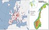 |
Fig. 1. Geographic distribution of the near real-time GNSS networks of EUREF (http://www.epncb.oma.be/) in the left panel and of the Norwegian RTK positioning network including EGNOS stations in the right panel. |
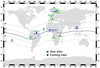 |
Fig. 2. Geographic distribution of the MONITOR GNSS station network. |
A unique opportunity enabling near real-time (NRT) monitoring of global TEC is offered by IGS via the Real-Time Pilot Project (RTPP – http://www.rtigs.net/pilot/index.php). Globally measured NRT data (1s streaming mode) are reliably distributed via the Federal Agency for Cartography and Geodesy (BKG) Frankfurt in Europe using the Networked Transport of RTCM via Internet Protocol (NTRIP) technology (http://igs.bkg.bund.de/ntrip/docu).
Since geodetic networks are not routinely equipped with high rate receivers, special efforts are made at various places in Europe to install individual or coordinated GNSS receivers capable of measuring radio scintillations at sampling rates of at least 20 Hz (see Table 1).
Location of high rate GNSS receivers installed by European institutions.
Such special networks contribute to international projects such as MONITOR/ESA (http://www.dlr.de/kn/en/desktopdefault.aspx/tabid-4307/6939_read-31000/admin-1/) and TRANSMIT/EC (http://www.transmit-ionosphere.net/transmit/index.aspx). Within the ESA project MONITOR a global scintillation monitoring network is established by using GPS and specifically developed Galileo receivers (see Fig. 2). The network will be operated via a Central Archiving and Processing Facility at ESTEC.
In addition to the publicly available geodetic networks, specific GNSS networks of European companies, governmental offices and research facilities, the European Geostationary Navigation Overlay Service (EGNOS) operates at present in 34 Ranging and Integrity Monitoring Stations (RIMS) which send the measured data to the Master Control Centre (MCC). Here the ionospheric corrections are computed and subsequently uplinked to geostationary satellites from where they are distributed to the users. Via the EGNOS Message Server (EMS) the EGNOS messages are accessible free-of-charge, using standard means. EMS stores the augmentation messages broadcast by EGNOS in hourly text files which can be used in other applications.
The EGNOS signal is encoded according to the Radio Technical Commission for Aeronautics (RTCA) in the DO-229D document (http://www.rtca.org/onlinecart/product.cfm?id=396). In middle latitudes the gridded values are spaced by 5° × 5° in latitude and longitude, respectively, whereas at high latitudes the spacing grows up to 30°.
NRT ionospheric data such as TEC and derived products are provided also by other services in Europe. Thus, the “Space Weather Application Center Ionosphere” (SWACI – http://swaciweb.dlr.de) provides European as well as global TEC maps with an update rate of 5 min (Jakowski et al., 2011). In addition to ground-based data, also space-based ionospheric data as TEC and electron density derived from radio occultation and navigation measurements are provided. In close cooperation with GFZ Potsdam satellite missions such as CHAMP, GRACE, Tandem-X, TerraSAR-X and SWARM are/will be exploited. Besides GNSS data also radio beacon measurements and vertical sounding data from Tromsø/Norway, Juliusruh/Germany and Průhonice/Czech Republic are used. In cooperation with the Tromsø Geophysical Observatory, the IAP Kuehlungsborn and the AIP Prague, we derive the equivalent slab thickness over these ionosonde stations in NRT. High rate data for analysing radio scintillations are obtained from a meridional chain of GNSS stations (see Table 1) providing scintillation monitor data about every 3 min.
The Istituto Nazionale di Geofisica e Vulcanologia in Rome/Italy operates the Service “electronic Space weather upper atmosphere” (eSWua) (Romano et al. 2008).
The eSWua (http://www.eswua.ingv.it) is a hardware-software system based on the upper atmosphere monitoring stations (ground-based GNSS receivers and ionosondes) managed by Istituto Nazionale di Geofisica e Vulcanologia. Through the web tools of the database (DB) designed for TEC and scintillations data, it is possible to visualize, plot, extract and download the data of each station operating in polar regions (Arctic and Antarctica), in the Mediterranean region (Crete/Greece and Lampedusa/Italy) and in Latin America (Tucuman/Argentina) as seen in Table 1. In addition to this the system hosts three University of Nottingham GISTM stations: Nottingham, Trondheim and Dourbes.
The Norwegian Mapping Authority (NMA) will launch a publicly available ionosphere monitoring service in 2012. The service is based on data from its own GNSS receiver network. Information about VTEC and small-scale perturbations will be available in NRT.
It should be mentioned that also other European research institutes such as the Universitat Politècnica de Catalunya (http://g1.upc.es/tomion/real-time/), University of Bath (http://www.bath.ac.uk/elec-eng/invert/iono/rti.html) and University of Warmia and Mazury Olsztyn provide GNSS-based ionospheric information in NRT.
All these services contribute to get a comprehensive view on the complex ionospheric processes. This idea is underlined in the FP7 project ESPAS where, for instance, vertical sounding and GNSS data shall be combined on European level. Thus, new data types are created which offer new insights into the generation, propagation and dissipation of ionospheric perturbations in relation to other space weather factors considered in COST ES0803.
2.2. Space-based GNSS measurements
Space-based GPS measurements onboard Low Earth Orbiting (LEO) satellites may essentially contribute to detect space weather effects in the Geo-plasma. Thus, Low Earth Orbiting (LEO) satellites are capable of monitoring the vertical ionization of the ionosphere on global scale (e.g., Hajj & Romans 1998; Jakowski 2005).
In addition to these measurements the navigation data can effectively be used to monitor the 3D electron density distribution of the topside ionosphere/plasmasphere near the orbit plane (Heise et al. 2002). The effectiveness of radio occultation measurements has been demonstrated by several satellite missions such as Microlab-1 with the GPS/MET experiment (Hajj & Romans 1998), SAC-C (https://directory.eoportal.org/web/eoportal/satellite-missions/s/sac-c), CHAMP (Reigber et al. 2000) and GRACE (Wickert et al. 2009).
As illustrated in Figure 3, the retrieved vertical electron density profiles from radio occultation as well as the topside electron density reconstructions are very helpful to understand the mechanism of ionospheric storms (e.g., Jakowski et al. 2007).
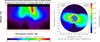 |
Fig. 3. Averaged 2D-ionosphere electron density distribution derived from radio occultation measurements in 2003 (left panel, Jakowski et al. 2007) and topside ionosphere/plasmasphere reconstruction of the electron density near the satellite orbital plane derived from navigation data onboard GRACE on day 337 in 2011 (right panel). |
3. Monitoring and tracking of ionospheric perturbations
3.1. Large-scale storms
Due to the strong electrodynamic coupling with the magnetosphere and the solar wind, enhanced space weather impact is expected in particular on the high-latitude ionosphere. The strong enhancements of the solar wind energy generate large perturbations in the high-latitude ionosphere and thermosphere resulting in significant variability of the plasma density and perturbation propagation towards lower latitudes.
A severe ionospheric storm was globally observed during the end of October 2003, called Halloween storm. The storm was initiated by a huge solar flare of class X17 on 28 October followed by two coronal mass ejections on subsequent days. The total electron content increased rapidly by more than 10 TECU (1 TECU = 1 × 10¹⁶ m−2) on 28 October at 11:05 UT (see Sect. 3.4).
When the CME coupled into the Earth’s magnetosphere, the generated convection electric field mapped down to the ionosphere and moved the plasma over the pole from the dayside to the night side via E × B drift. The plasma drift is upward directed at lower latitudes thus causing an enhancement of TEC. Both effects can be nicely seen in Figure 4, left panel, by the enhanced TEC level forming a tongue of ionization over the North Pole.
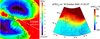 |
Fig. 4. Topside TEC measurements from CHAMP on 29 October 2003 around 8:00 UT (left panel, Jakowski et al. 2009) and storm pattern (deviations from monthly medians) of ground-based TEC on 30 October at 21:30 UT. The white line at the left panel indicates the CHAMP orbit plane. |
On the next day the TEC perturbation deviations from the corresponding monthly median TEC level reach more than 200% as can be seen in Figure 4, right panel.
The related perturbation pattern maps are quite useful for studying general features of ionospheric storm generation and propagation. The ionization front and related perturbation pattern can be detected and traced by more adequate techniques such as wavelet analysis (cf. Borries et al. 2009). Here the propagation is mostly southward. Velocities of perturbations may be estimated by tracing these perturbations as illustrated in Figure 5. Here deviations from mean behaviour are used to visualize transport of ionization towards the south in the space-time diagram. The storm pattern propagates equatorward with velocities in the order of about 600 m/s. Direction and velocity of these perturbation can effectively be used to forecast ionospheric perturbations after they have been reliably detected at high latitudes, for example, within the Norwegian RTK positioning network.
 |
Fig. 5. TID storm pattern observed at the Halloween storm on 29 October 2003 showing different perturbation propagation effects (Jakowski et al. 2009). |
The TID storm pattern seen in Figure 5 indicates quite different processes such as the instantaneous enhancement throughout all latitudes considered here at about 6:30 UT. This is due to the immediate action of the convection electric field before the ring current has been developed. From 58° N towards the North Pole we see the trace of the tongue of ionization seen also in Figure 4 as discussed before. Later we see a number of perturbation traces propagating towards Southern Europe. The slopes indicate velocities in the order of 600 m/s typically for large-scale perturbation pattern (e.g., Borries et al. 2009). In the afternoon around 15:00 UT starts the equatorward motion of the high-latitude trough which separates polar patches in the north from more regular transport processes in the south. The propagation velocity of the trough motion is in the order of about 50 m/s.
As indicated in a former study of COST 276 activity including European vertical sounding stations, the horizontal gradients of ionospheric ionization showed an azimuthal asymmetry pronouncing the North-South direction on average (Jakowski et al. 2008).
Taking into account the complexity of ionospheric storms, statistical as well as case studies contribute to explore the mechanism of ionospheric perturbations. Although each ionospheric storm has its individual face, there are some common features which can be separated in statistical studies (e.g., Foerster & Jakowski 2000; Borries et al. 2009). To separate perturbation induced changes of TEC from regular behaviour, differential TEC maps presenting the deviation from mean or median reference values can effectively be used. Thus, the percentage deviation (ΔTEC = (TEC − TECmed)/TECmed × 100) is quite useful for studying general features of ionospheric storms (e.g., Jakowski et al. 1999; Foerster & Jakowski 2000).
The immediate response of TEC at storm onset, as shown in Figure 5 at 06:30 UT, is a typical phenomenon which becomes clearly visible when strong storms with a well-defined onset are superposed (Arbesser-Rastburg & Jakowski 2007). In that case the storm onset was defined by a rapid increase of the geomagnetic Dst index (ΔDst/Δt > 10 nT/hour) before the main storm phase starts with a strong depression of Dst.
Another typical feature is the development of the “tongue of ionization” which indicates a huge plasma transport across the pole from the dayside towards the night side as shown in Figure 4, left panel. Since the tongue of ionization is driven by the space weather induced convection electric field, it is closely associated with one of the main storm driving forces. The strong plasma drift is often related to other ionospheric irregularities as discussed in subsequent sections. Besides electric fields also perturbation induced neutral winds have a strong impact on plasma motion (e.g., Prölss 1995). Perturbation induced equatorward blowing meridional winds are most effective to lift up the plasma along geomagnetic field lines in mid-latitudes. As pointed out by Foerster & Jakowski (2000) the interference with the global thermospheric wind system might lead to seasonal differences in the averaged storm pattern.
It can be concluded that the described individual Halloween storm pattern reflects common features of severe ionospheric storms.
3.2. Medium-scale travelling ionospheric disturbances (MSTIDs)
The MSTIDs are ionospheric signatures of atmospheric waves, up to few TECUs of amplitude at solar cycle maximum conditions. They propagate with typical periods ranging from several minutes to somewhat less than 1 h at velocities from 50 to 300 m/s (e.g., Hernandez-Pajares et al. 2006). In spite of some authors using the MSTID term to refer only to a subset of them (those occurring during night and local winter and moving westward, see, Kelley 2011, or Beach et al. 1997), we will keep the original scope for the MSTID term, which includes all of ionospheric wave signatures fitting in the aforementioned range of velocities and periods. In particular, MSTIDs occurring at local day time and winter, moving equatorward probably due to classical Atmospheric Gravity Wave (AGW) interaction with the ionosphere (Kelley 2011), are also considered in such term.
The origin of MSTIDs is not well established yet, but several potential sources have been identified:
-
The neutral atmosphere turbulence associated to meteorological activity and atmospheric winds (see Bertin et al. 1978; Van Velthoven 1990 and Scotto 1995).
-
The vertical irradiance gradient associated to the Solar Terminator (ST) at the given ionospheric region and its magnetic conjugate region, which seems to be a solid candidate to explain most part of the MSTID climatology (e.g., Hernandez-Pajares et al. 2006; Afraimovich et al. 2009).
-
The Perkins instability, which would make understandable, in terms of the weakest damping direction, the preferred westward propagation of local winter MSTIDs at night (Kelley 2011).
Different techniques and applications, such as precise GNSS navigation and VLBI, are sensitive to the MSTIDs effect at mid-latitudes, appearing as small electron content gradients (up to few TECU) at length scales of half MSTID wavelengths, typically ranging from 50 to 300 km. This effect frequently occurs due to the above-mentioned typical MSTID occurrence probability (during fall/winter mainly at day time versus spring/summer at night time). Taking into account this behaviour, they can be modelled and mitigated (e.g., Hernandez-Pajares et al. 2012). In this context, one very recent result (Hernandez-Pajares et al. 2012) consists in the possibility to extrapolate (to great extent) mid-latitude MSTID characteristics to high and low latitudes. This finding has been possible thanks to the detailed study of the longest available period of most recent local networks of dual-frequency GPS data (from 4 to 13 years) at Alaska (AS), Hawaii (HW), California (CA) and New Zealand (NZ). In Figure 6 it can be seen that the equatorward propagation of MSTIDs is at about 100–300 m/s during local noon-time and winter season affecting the four local networks at high, low and north- and south-mid-latitudes respectively.
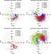 |
Fig. 6. Polar plots representing MSTID velocities (m/s) and azimuths for local fall, for the four selected networks, AS (top-left), CA (top-right), HW (bottom-left) and NZ (bottom-right), in the analysed period. Colour code: black for LT 00–04 h, light blue for LT 04–08 h, dark blue for LT 08–12 h, red for LT 12–16 h, green for LT 16–20 h and grey for LT 20–24 h (Figure extracted from Hernandez-Pajares et al. 2012). |
When considering smaller scales than those typically for the observation of MSTIDs, the wave-like character of perturbations is lost and irregular behaviour of perturbations dominates as considered in the next chapter.
3.3. Small-scale ionospheric perturbations causing radio scintillations
The project “Ionospheric Scintillations Arctic Campaign Coordinated Observation (ISACCO)” was born in 2003 when the first GISTM receiver (GPS Ionospheric and TEC Monitor) was deployed at Dirigibile Italia Station (Ny Alesund-Svalbard, Norway; De Franceschi et al. 2006). Currently INGV manages a TEC and scintillation monitoring network at polar, mid- and low latitudes (see Table 1). As the establishment of the monitoring network, the idea came out to develop an original technique allowing the identification of areas of the ionosphere in which scintillation is more likely to occur (Spogli et al. 2009, 2010). Combining this technique, based on a suitable statistical treatment and representation of the scintillation data, with TEC maps as obtained by MIDAS (Multi-Instrument Data Analysis System; Spencer & Mitchell 2007), the effects of the severe October/November 2003 storms over the North polar ionosphere and Northern Europe have been investigated (De Franceschi et al. 2008). Through MIDAS the plasma dynamics was reconstructed and high TEC “islands” identified over Northern Europe, more likely originated from the convection of plasma from the North American region. Storm-related plasma convection is characterized by the presence of F-region electron density patches. In fact, severe amplitude and phase scintillations were observed in coincidence with steep TEC gradients, a characteristic of the edge of polar cap patches (Fig. 7). These gradients can result in the production of small-scale irregularities by the gradient-drift instability.
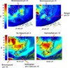 |
Fig. 7. Equivalent vertical TEC (TECU) snapshots by MIDAS for 30 October 2003 at 21:40 and 22:25 UT (top), and 20 November 2003 at 19:10 and 19:50 UT (bottom). Phase scintillation index maxima for selected PRNs from the GISTM network chain are superimposed (adapted from De Franceschi et al. 2008). |
The multi-instrument approach was successfully used to investigate the moderate storm which occurred on early April 2006 at equatorial latitude (Alfonsi et al. 2011). The study highlighted the ionospheric conditions leading to scintillation events and the phenomenon of amplitude scintillation inhibition. Moreover, the simultaneous use of the amplitude scintillation index S4, ROT (rate of TEC change) and ROTI (rate of TEC index) helped in identifying the scale size of the irregularities leading to scintillation in the range between the order of 10 kilometres down to less than hundreds of metres.
3.4. Sudden increases of total electron content (SITECs)
SITEC measurements have been performed many years ago mainly based on Faraday rotation measurements at linearly polarized beacon signals from geostationary satellites such as ATS 6 (e.g., Davies 1980). Nowadays GNSS measurements are well suited to measure flare-related ionization events.
Coinciding with the approach to the 24th solar cycle expected maximum, the interest for a better observation capability of the increasing solar flare events, considered as space weather precursors, has grown significantly. In particular, better accuracy and temporal resolution of the changes within the flux of photons are becoming important to get a better understanding of the Sun-Earth relationships (Woods et al. 2011).
Solar flares are sudden electromagnetic over-emissions, which are often associated with explosive events on the Sun surface releasing huge amounts of magnetic energy and charged particles. They are characterized by the emission of radiation across the whole electromagnetic spectrum, especially in X-rays and Extreme Ultraviolet (EUV) bands, and by the ejection of energetic particles. On one hand, the radiation photons related to a solar flare facing the Earth produce a sudden over-ionization only in the daylight ionosphere that can be approximated by the Chapman model, predicting a dependence on the solar-zenith angle (SZA or χ; see Mendillo et al. 1974). On the other hand, the arrival time at Earth of the accelerated energetic particles (Solar Energetic Particles, SEPs and Energetic Storm Particles, ESPs) is delayed by even days with respect to photons (Tsurutani et al. 2009). Regarding near-relativistic electrons, a median delay of about 10 min is also observed (Haggerty & Roelof 2002). Note that the energetic particles can enter the Earth through the polar caps and affect the high and middle latitude ionosphere. In such case, the increase of ionization would not be dependent on the SZA and would also disturb the night-side ionosphere.
In summary, the EUV, X-ray and gamma rays are the primary ionization source in the Earth’s ionosphere. In this way, monitoring their sudden over-ionization effect, in terms of the ionospheric TEC (see Fig. 8), becomes not only a useful way to detect solar flare photons facing the Earth, but also an accurate way of measuring quick flare EUV photon flux increases (e.g., Garcia-Rigo et al. 2007).
 |
Fig. 8. De-trended VTEC rate versus cosine of solar zenith angle, for three representative solar flares, with decreasing intensity; from top to bottom: day 301 of 2003, precursor flare of Halloween storm (X17.2 flare, day 301, 2003, 39777 s of GPS time), M9.3 flare, day 216 of 2011 (13908 s of GPS time) and C3.9 flare, day 210 of 2011 (44134 s of GPS time). The corresponding regression lines and 1-sigma boundaries are given. |
3.5. Overall perturbation degree
After reviewing ionospheric perturbations at different scales in the previous sections, the question arises how the perturbation degree of the ionosphere can reliably be measured for scientific research and practical applications in a more general way. As discussed before, ionospheric perturbations are due to complex coupling processes in the magnetosphere, thermosphere, ionosphere and upper atmosphere. Thus, to characterize the perturbation degree of the ionosphere by geomagnetic indices is restricted. Hence, some attempts have been made in recent years to develop a perturbation index that is easy to handle on the one side and characterizes the physical state of the ionosphere appropriately on the other side (Jakowski et al. 2012). Thus, in order to characterize large- and middle-scale ionospheric perturbations, the concept of a Disturbance Ionosphere Index (DIX) has been developed (Jakowski et al. 2012). Taking into account the existence of dense GNSS networks as described in Section 2 and to avoid calibration problems when estimating TEC, the index is based simply on relative TEC estimations obtained from differential GNSS carrier phases. To separate temporal and spatial information, the TEC rates at the ionospheric piercing points of two radio links are considered. Since solar radiation bursts illuminate large areas, the difference of both TEC rates is practically free from solar radiation effects if the ray paths are not too far away from each other. Thus, the difference is assumed to provide spatial information whereas the averaged sum of both TEC rates pronounces solar irradiation effects.
A preliminary version of this index has been temporarily provided via SWACI. Subsequent studies shall prove whether there is a potential for using such an index in research and NRT applications. A DIX sample is shown in Figure 9 for the 26 September 2011.
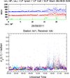 |
Fig. 9. High-latitude Disturbance Index (DIX) on 26 September 2011 in comparison with phase scintillation measurements at Kiruna GNSS station (see Table 1). |
When reaching the Earth in the evening hours of 26 September, the space weather event caused considerable ionospheric perturbations which are seen in DIX computed for the latitude range 55–65° N at three different longitudinal sectors.
As it can be seen in Figure 9, enhanced DIX values may be strongly correlated with scintillation activity. Since DIX is defined as a physics-based index, there is a capability to forecast DIX if other space weather factors and their impact are well known. DIX may be adapted to practical needs, for example, by defining a specific region and time and space resolution.
Since perturbation pattern (deviations from reference values such as medians) as discussed in Section 3.1 in relation to Figures 3 and 4 contains information on the strength of the perturbation, such information can also be used for characterizing ionospheric storms, for example, at each grid point of a service area. Such information, called W-index, is provided online at the Regional Warning Center (RWC) Warsaw under http://www.cbk.waw.pl/ and archived for comparison with W-index maps derived from the global ionospheric maps, GIM.
The degree of perturbation, DTEC, is computed as log of TEC relative to quiet reference median for 27 days prior to the day of observation. The W-index map is generated by segmentation of DTEC with the relevant thresholds specified earlier for foF2 so that 1 or −1 stands for the quiet state, 2 or −2 for the moderate disturbance, 3 or −3 for the moderate ionospheric storm and 4 or −4 for intense ionospheric storm at each grid point of the map (Fig. 10). The planetary ionospheric storm Wp index is obtained from the W-index map as a latitudinal average of the distance between maximum positive and minimum negative W-index weighted by the latitude/longitude extent of the extreme values on the map. The threshold Wp exceeding 4.0 index units and the peak value Wpmax ≥ 6.0 specify the duration and the power of the planetary ionosphere-plasmasphere storm. It is shown that the occurrence of the Wp storms is growing with the phase of the solar cycle being twice as much as the number of magnetospheric storms with Dst ≤ −100 nT and Ap ≥ 100 nT.
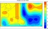 |
Fig. 10. W-index for European area calculated for 31 January 2011 5 UT based on TEC derived from EGNOS message. |
4. Forecasting ionospheric behaviour
Space weather studies as coordinated in COST action ES0803 shall give us an improved understanding of the physics behind space weather phenomena in order to better forecast space weather related effects and their impact on technical systems.
The GNSS user community is interested in forecasts of ionospheric perturbations. The regular ionospheric behaviour is described by empirical models such as IRI or NeQuick. Since reliable forecasts of ionospheric storms require not only a comprehensive understanding of the coupling of solar wind into the magnetosphere, thermosphere and ionosphere systems but also related data, we are far away from reliably predicting ionospheric perturbations. Nevertheless, there are some international efforts to improve forecasting of large-scale ionospheric perturbations. TEC map forecasts of 1 h ahead are made routinely via SWACI service based on current ionospheric behaviour and a background model (Jakowski et al. 2011). One hour after the forecast has been released, the forecast is compared with the measured TEC map. The corresponding difference plot is available for users allowing immediately estimating the quality of the forecast (see Fig. 11). Forecast errors are usually less than 10% of the original values.
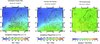 |
Fig. 11. TEC maps over Europe on 22 April 2012, 14:45 UT as provided via SWACI. Actual TEC map (left panel), 1 h TEC forecast for Europe (middle), quality of forecast provided immediately after computing the actual TEC map (right panel). |
To forecast ionospheric storms several hours ahead, the storm development from the sun via the magnetosphere and thermosphere to the ionosphere must be tracked continuously. This is a challenging task which is especially considered in the FP7 project AFFECTS (http://www.affects-fp7.eu/).
Small-scale irregularities causing radio scintillations are commonly described by statistical methods. In Europe two major empirical models describing scintillation occurrence probability have been developed.
In GNSS positioning a simplified stochastic model is often used which assumes that all the GNSS observables are statistically independent and of the same quality. To mitigate the scintillation impact on positioning, Aquino et al. (2009) suggested the computation of different weights derived from the scintillation-sensitive receiver tacking models of Conker et al. (2003). This approach has been successfully adopted by Alves da Silva et al. (2010): data from the GISTM network in Northern Europe were processed in both relative and point positioning modes showing improvements of the order of 45%–50% in height accuracy when the modified stochastic model is applied under moderate to strong scintillation conditions. The proposed mitigation solution could make use of suitable scintillation models instead of using GISTM experimental data (50 Hz) to be effective against the ionospheric scintillations.
A very promising investigation in this sense has been recently made in the frame of the CIGALA FP7-Project (Sreeja et al. 2011): the WAM model (Wernik et al. 2007), previously developed at high latitude, and has been tuned to model the equatorial scintillation scenario in the Latin American longitudinal sector to support the improvement of tracking models. The input data to the WAM model are DE2 (Dynamic Explorer 2) retarding potential analyser (RPA) measurements of the ion density. The new version of WAM will reproduce statistically well the climatology of scintillations on a diurnal and seasonal basis as obtained by comparing WAM output with experimental data from the CIGALA network (Sreeja et al. 2011). Its limitations when used as a prediction model for specific satellite-receiver links are however apparent and need deeper investigations. This is mainly due to the fact that WAM results depend on the available spatial/temporal coverage of the in situ measurements that are sparse and non-uniformly distributed at the equatorial region.
The Global Ionospheric Scintillation Propagation Model (GISM) has been developed concurrently to several measurement campaigns under ESA/ESTEC initiatives (Béniguel et al. 2009, Prieto Cerdeira & Beniguel 2011). It uses the Multiple Phase Screen (MPS) technique (Béniguel & Hamel 2011). The locations of transmitters and receivers are arbitrary. The incidence link angle is arbitrary regarding the ionosphere layers and the magnetic field vector orientation. It can cross the entire ionosphere or a small part of it. At each screen location along the line of sight, the parabolic equation (PE) is solved. GISM allows calculating mean errors and scintillations due to propagation through the ionosphere. Recent developments allow calculating the two positions – two frequencies mutual coherence scattering function for radar observations. This model is accessible online at http://www.ieea.fr/en/gism-web-interface.html. Modelling results shall be compared versus measurements at a number of GNSS stations as seen in Figure 2. Samples of modelling results are given in Figure 12.
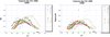 |
Fig. 12. Intensity and phase scintillation indices on day 314, GPS week No 377, 2006 obtained by GISM modelling. Colours correspond with GPS satellite numbers (PRN). |
5. Ionospheric impact and use of ionospheric perturbation information in GNSS applications
Ionospheric perturbations have a strong impact in particular on precise and Safety of Life (SoL) GNSS applications. Thus, detection, tracking and forecasting of ionospheric perturbations is a challenging task that can only be solved in close dialogue with the user community. In this section we briefly discuss ionospheric impact on GNSS to underline the necessity to continue consequently research activities reported in this paper.
Since ionospheric large- and medium-scale perturbations are generated predominantly at high latitudes, GNSS applications are impacted in particular at high latitudes. Measurements of ionospheric disturbances and positioning network performance during geomagnetic activity in Norway have shown that the northern part of the network is frequently disturbed, even during minor space weather events. For stronger events, the disturbances are seen also at lower latitudes. In Figure 13 an example of network disturbances is demonstrated.
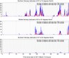 |
Fig. 13. Sample for the performance degradation of Norwegian geodetic network during the moderate storm on 10/11 March 2011. |
Besides space weather driven large-scale storm effects, also medium-scale perturbations affect precise positioning as already indicated in Section 3.2. The recent years have seen the development of GNSS dense networks allowing the users to compute their position with centimetre-level accuracy in real time, thanks to the Real-Time Kinematics technique (RTK).
Generally, RTK users expecting cm accuracy are not aware of the threat due to the presence of ionospheric irregularities. As shown by Lejeune et al. (2012), ionospheric positioning error during the occurrence of an MSTID can reach about 25 cm for a 25 km baseline.
Taking into account the preferred orientation of MSTID propagation as discussed in Section 3.2, Lejeune et al. (2012) propose to assess the influence of baseline orientation on the positioning error due to the ionosphere. MSTIDs being moving structures, their effect in terms of positioning error varies with the baseline orientation. As a matter of example, if a given baseline is oriented perpendicular to the MSTID direction of propagation (parallel to the wave front), its related positioning error will be weaker than that observed for a baseline oriented parallel to the propagation direction, due to larger TEC gradients in the latter case. Based on a network of 60 dual-frequency GNSS stations in Belgium (for a total of about 160 baselines), the authors have analysed a typical winter daytime MSTID case. The standard deviation (SD) of the positioning error σpos has been reported as a function of baseline azimuth during the occurrence of the structure (1000–1500 LT), as shown in Figure 14. Network baselines showing all different lengths (from 4 to 40 km), σpos values have been standardized by the baseline length to allow comparisons. The polar plot of Figure 14 (left) exhibits a rather anisotropic pattern, what allows identifying the MSTID direction of propagation (i.e., mostly equatorward). In another example taken 7 years later, similar results have been obtained for the same type of structure (winter/daytime MSTID), despite a more pronounced westward component, clearly visible in Figure 14 (right).
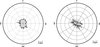 |
Fig. 14. Polar plots of σpos normalized by baseline length for DOY 359/04 (left) and DOY 345/11 (right) in the Active Geodetic Network (AGN), Belgium. |
The ionospheric positioning error is monitored over the whole Belgian RTK network including 60 GNSS stations. Every 15 min, an activity index is assigned to each baseline and the latter is mapped, following a colour scale ranging from green (quiet conditions) to red (extreme conditions). As network maps are created every 15 min, the service allows a precise identification of the disturbed periods. It is planned to establish a NRT service by ULg for providing this information on a routine basis.
Besides performance degradation of precise geodetic networks, also SoL services of Space-Based Augmentation Systems (SBAS) such as WAAS and EGNOS suffer from ionospheric perturbations. In case of aircraft landing, enhanced horizontal gradients of TEC may cause violation of protection levels defined to guarantee safe landing procedure (e.g., Mayer et al. 2009). EGNOS entered into operation for Safety of Life in March 2011. Due to the fact that the used geostationary satellites already cover Europe and the entire African continent, EGNOS could easily extend the service provision to the African continent resulting in an increase in the overall safety of air transport. In order to explore regional extension models for EGNOS towards South Africa, the ESESA (EGNOS Service Extension to South Africa) project has been established. Considering the crest region and related gradients at both sides of the geomagnetic equator associated with enhanced plasma instabilities near the geomagnetic equator (e.g., Béniguel et al. 2009; Béniguel & Hamel 2011), this is a great challenge for monitoring and modelling ionospheric perturbations and scintillations.
6. Summary and conclusions
The paper has demonstrated that space weather events may cause severe perturbations of ionospheric behaviour. Since the dynamics and the ionospheric structure at practically all geometric scales impact transionospheric radio waves at the L band significantly, GNSS users have to be aware of space weather impact.
Fortunately, the data basis has grown considerably in recent years. Thanks to a rather dense geodetic network in Europe there is a unique capability to monitor the Total Electron Content by dual-frequency GNSS measurements automatically in NRT. Space-based GNSS measurements onboard LEO satellites can essentially contribute to study solar-terrestrial relationships and to model the ionosphere under perturbed conditions. Due to delayed data download these measurements cannot be used yet for NRT services having a latency of less than 1 h. Nevertheless, these data are still attractive to be used as input in physics-based forecast models needed to be developed in Europe in the future.
Although considerable progress has been achieved in recent years, model development must continue. Current use of empirical models to forecast ionospheric perturbations needs further improvements concerning the full spectrum of space weather information. The quality of ionospheric predictions depends on the quality of input data such as forecasted solar irradiance, solar wind and geomagnetic activity.
The availability of ionospheric perturbation indices currently under development will enhance the acceptance of GNSS-based ionospheric data services at user level.
A number of international projects supported by ESA and EC are established to further improve our capabilities to monitor, track and forecast ionospheric perturbations. COST activity ES0803 has essentially contributed to support international collaboration, coordinating measurement campaigns and initiating space weather related international projects.
Acknowledgments
The authors thank the geodetic community, i.e., IGS, EUREF and national GNSS networks for making available high-quality GNSS data. We are grateful to COST action ES0803 for initiating, coordinating and supporting collaboration within international projects. Arctic and Antarctic GNSS network ISACCO is partially supported by PNRA (Programma Nazionale di Ricerche in Antartide). Finally, we thank also our co-workers for their assistance in preparing this review.
References
- Afraimovich, E.L., I.K. Edemskiy, A.S. Leonovich, L.A. Leonovich, L.A. Leonovich, S.V. Voeykov, and Y.V. Yasyukevich, MHD nature of night-time MSTIDs excited by solar terminator, Geophys. Res. Lett., 36, L15106, 1–5, DOI: 10.1029/2009GL039803, 2009. [Google Scholar]
- Alfonsi, Lu., G. De Franceschi, V. Romano, A. Bourdillon, and M. Le Huy, GPS scintillations and TEC gradients at equatorial latitudes on April 2006, Adv. Space Res., 47, 1750–1757, 2011. [Google Scholar]
- Alves da Silva, H., P. Camargo, J.F. Galera Monico, M. Aquino, H.A. Marques, G.G. De Franceschi, and A. Dodson, Stochastic modelling considering ionospheric scintillation effects on GNSS relative and point positioning, Adv. Space Res., 45, 1113–1121, 2010. [Google Scholar]
- Aquino, M., J.F.G. Monico, A.H. Dodson, H.A. Marques, G. De Franceschi, L. Alfonsi, V. Romano, and M. Andreotti, Improving the GNSS positioning stochastic model in the presence of ionospheric scintillation, J. Geod., DOI: 10.1007/s00190-009-0313-6, 2009. [Google Scholar]
- Arbesser-Rastburg, B., and N. Jakowski, Effects on Satellite Navigation in Space weather, physics and effects, Eds. V., Bothmer, and J. Daglis. Springer, Heidelberg, 383–402, 2007. [CrossRef] [Google Scholar]
- Beach, T.L., M.C. Kelley, P.M. Kintner, and C.A. Miller, Total electron content variations due to nonclassical traveling ionospheric disturbances: Theory and Global Positioning System observations, J. Geophys. Res., 102 (A4), 7279–7292, DOI: 10.1029/96JA02542, 1997. [CrossRef] [Google Scholar]
- Béniguel, Y., J-P Adam, N. Jakowski, T. Noack, V. Wilken, J.-J. Valette, M. Cueto, A. Bourdillon, P. Lassudrie-Duchesne, and B. Arbesser-Rastburg, Analysis of scintillation recorded during the PRIS measurement campaign, Radio Sci., 44, DOI: 10.1029/2008RS004090, 2009. [Google Scholar]
- Béniguel, Y., and P. Hamel, A global ionosphere scintillation propagation model for equatorial regions, J. Space Weather Space Clim., 1 (2011), DOI: 10.1051/swsc/2011004, 2011. [Google Scholar]
- Bertin, F., J. Testud, L. Kersley, and P.R. Rees, The meteorological jet stream as a source of medium scale gravity waves in the thermosphere – an experimental study, J. Atmos. Terr. Phys., 40, 1161–1183, 1978. [CrossRef] [Google Scholar]
- Borries, C., N. Jakowski, and V. Wilken, Storm induced large scale TIDs observed in GPS derived TEC, Ann. Geophys., 27 (4), 1605–1612, Copernicus Publications, ISSN 0992-7689, 2009. [Google Scholar]
- Conker, R.S., M.B. El-Arini, C.J. Hegarty, and T. Hsiao, Modeling the effects of ionospheric scintillation on GPS/satellite-based augmentation system availability, Radio Sci., 38 (1), DOI: 10.1029/2000RS002604, 2003. [CrossRef] [Google Scholar]
- Davies, K., Recent progress in satellite radio beacon studies with particular emphasis on the ATS-6 radio beacon experiment, Space Sci. Rev., 25, 357–430, 1980. [CrossRef] [Google Scholar]
- De Franceschi, G., L. Alfonsi, and V. Romano, ISACCO: an Italian project to monitor the high latitudes ionosphere by means of GPS receivers, GPS Solutions, 18, 263–267, DOI: 10.1007/s10291-006-0036-6, 2006. [CrossRef] [Google Scholar]
- De Franceschi, G., L. Alfonsi, V. Romano, M. Aquino, A. Dodson, C.N. Mitchell, and A.W. Wernik, Dynamics of high latitude patches and associated small scale irregularities, J. Atmos. Sol. Terr. Phys., 70 (6), 879–888, DOI: 10.1016/j.jastp.2007.05.018, 2008. [CrossRef] [Google Scholar]
- Foerster, M., and N. Jakowski, Geomagnetic storm effects on the topside ionosphere and plasmasphere: a compact tutorial and new results, Surv. Geophys, 21 (1), 47–87, 2000. [Google Scholar]
- Garcia-Rigo, A., M. Hernandez-Pajares, J.M. Juan, and J. Sanz, Solar flare detection system based on global positioning system data: First results, Adv. Space Res., 39, 2007. [Google Scholar]
- Haggerty, D.K., and E.C. Roelof, Impulsive near-relativistic solar electron events: delayed injection with respect to solar electromagnetic emission, Astrophys. J., 579, 841–853, 2002. [Google Scholar]
- Hajj, G.A., and L.J. Romans, Ionospheric electron density profiles obtained with the Global Positioning System: results from the GPS/MET experiment, Radio Sci., 33 (1), 175–190, 1998. [CrossRef] [Google Scholar]
- Heise, S., N. Jakowski, A. Wehrenpfennig, Ch. Reigber, and H. Lühr, Sounding of the topside ionosphere/plasmasphere based on GPS measurements from CHAMP: initial results, Geophys. Res. Lett., 29 (14), 44-1–44-4, DOI: 10.1029/2002GL014738, 2002. [Google Scholar]
- Hernandez-Pajares, M., J.M. Juan, and J. Sanz, Medium-scale traveling ionospheric disturbances affecting GPS measurements: Spatial and temporal analysis, J. Geophys. Res., 111, A07S11, DOI: 10.1029/2005JA011474, 2006. [Google Scholar]
- Hernandez-Pajares, M., J.M. Juan, J. Sanz, and A. Aragon-Angel, Propagation of medium scale travelling ionospheric disturbances at different latitudes and solar cycle conditions, Radio Sci., 47, RS0K05, DOI: 10.1029/2011RS004951, 2012. [CrossRef] [Google Scholar]
- Jakowski, N., S. Schlueter, and E. Sardon, Total Electron Content of the Ionosphere During the Geomagnetic Storm on January 10, 1997, J. Atmos. Solar-Terr. Phys., 61, 299–307, 1999. [CrossRef] [Google Scholar]
- Jakowski, N., Ionospheric GPS Radio Occultation measurements on board CHAMP, GPS Solutions, 9, 88–95, DOI: 10.1007/s10291-005-0137-7, 2005. [CrossRef] [Google Scholar]
- Jakowski, N., V. Wilken, and C. Mayer, Space weather monitoring by GPS measurements on board CHAMP, Space Weather, 5, S08006, DOI: 10.1029/2006SW000271, 2007. [CrossRef] [Google Scholar]
- Jakowski, N., J. Mielich, C. Borries, L. Cander, A. Krankowski, B. Nava, and S.M. Stankov, Large scale ionospheric gradients over Europe observed in October 2003, J. Atmos. Sol. Terr. Phys., DOI: 10.1016/j.jastp.2008.03.020, 2008. [Google Scholar]
- Jakowski, N., C. Mayer, C. Borries, and V. Wilken, Space weather monitoring by ground and space based GNSS measurements, Proc. ION – International Technical Meeting, January 26–28, Anaheim, CA, 2009. [Google Scholar]
- Jakowski, N., C. Mayer, M.M. Hoque, and V. Wilken, TEC models and their use in ionosphere monitoring, Radio Sci., 46, RS0D18, DOI: 10.1029/2010RS004620, 2011. [CrossRef] [Google Scholar]
- Jakowski, N., C. Borries, and V. Wilken, Introducing a Disturbance Ionosphere Index (DIX), Radio Sci., DOI: 10.1029/2011RS004939, 2012. [Google Scholar]
- Kelley., M.C., On the origin of mesoscale TIDs at midlatitudes, Ann. Geophys., 29, 361–366, 2011. [Google Scholar]
- Lejeune, S., G. Wautelet, and R. Warnant, Ionospheric effects on relative positioning within a dense GPS network, GPS Solutions, 16 (1), 105–116, 2012. [CrossRef] [Google Scholar]
- Mayer, C., B. Belabbas, N. Jakowski, M. Meurer, and W. Dunkel, Ionosphere Threat Space Model Assessment for GBAS, ION GNSS 2009, 22–25 September, Savannah, GA, USA, 2009. [Google Scholar]
- Mendillo, M., J.A. Klobuchar, R.B. Fritz, A.V. Da Rosa, L. Kersley, et al., Behavior of the ionospheric F region during the great solar flare of August 7, 1972, J. Geophys. Res., 79, 665–672, 1974. [Google Scholar]
- Prieto Cerdeira, R., and Y. Beniguel, The MONITOR project: architecture, data and products, Ionospheric Effects Symposium, Alexandria VA, 2011. [Google Scholar]
- Prölss, G.W., Ionospheric F-region storms, in Handbook of Atmospheric Electrodynamics, Ed. H. Volland, CRC Press, Boca Raton, 2, 195–248, 1995. [Google Scholar]
- Reigber Ch., H. Lühr, and P. Schwintzer, CHAMP mission status and perspectives, Suppl. to EOS, Transactions, AGU, 81, 48, F307, 2000. [Google Scholar]
- Romano, V., S. Pau, M. Pezzopane, E. Zuccheretti, B. Zolesi, G. De Franceschi, and S. Locatelli, The electronic Space Weather upper atmosphere (eSWua) project at INGV: advancements and state of the art, Ann. Geophys., 26 (2), 345–351, 2008. [Google Scholar]
- Scotto, C., Sporadic-E layer and meteorological activity, Ann. Geofis., XXXVIII (1), 1995. [Google Scholar]
- Spencer, P.S.J., and C.N. Mitchell, Imaging of fast-moving electron density structures in the polar cap, Ann. Geophys., 50 (3), 427–434, 2007. [Google Scholar]
- Spogli, L., L. Alfonsi, G. De Franceschi, V. Romano, M.H.O. Aquino, and A. Dodson, Climatology of GPS ionospheric scintillations over high and mid-latitude European regions, Ann. Geophys., 27, 3429–3437, 2009. [CrossRef] [Google Scholar]
- Spogli, L., L. Alfonsi, G. De Franceschi, V. Romano, M. Aquino, and A. Dodson, Climatology of GNSS ionospheric scintillation at high and mid latitudes under different solar activity conditions, Il Nuovo Cimento, 125 B, 623–632, DOI: 10.1393/ncb/i2010-10857-7, 2010. [Google Scholar]
- Sreeja, V.V., M. Aquino, B. Forte, Z. Elmas, C. Hancock, et al., Tackling ionospheric scintillation threat to GNSS in Latin America, J. Space Weather Space Clim., 1, A05, DOI: 10.1051/swsc/2011005, 2011. [CrossRef] [EDP Sciences] [Google Scholar]
- Tsurutani, B.T., O.P. Verkhoglyadova, A.J. Mannucci, G.S. Lakhina, G. Li, and G.P. Zank, A brief review of solar flare effects on the ionosphere, Radio Sci., 44, RS0A17, DOI: 10.1029/2008RS004029, 2009. [CrossRef] [Google Scholar]
- Van Velthoven, P.J., Medium-scale irregularities in the ionospheric electron content, Ph.D. Thesis, Technische Universiteit Eindhoven,1990. [Google Scholar]
- Wernik, A.W., L. Alfonsi, and M. Materassi, Scintillation modeling using in situ data, Radio Sci., 42, RS1002, DOI: 10.1029/2006RS003512, 2007. [CrossRef] [Google Scholar]
- Wickert, J., G. Michalak, T. Schmidt, G. Beyerle, C.Z. Cheng, et al., GPS radio occultation: Results from CHAMP, GRACE and FORMOSAT-3/COSMIC, Terr. Atmos. Oceanic Sci., 20, 45–50, DOI: 10.3319/TAO.2007.12.26.01 (F3C), 2009. [CrossRef] [Google Scholar]
- Woods, T.N., R. Hock, F. Eparvier, A.R. Jones, P.C. Chamberlin, et al., New solar extreme-ultraviolet irradiance observations during flares, Astrophys. J., 739, 59, DOI: 10.1088/0004-637X/739/2/59, 2011. [Google Scholar]
Cite this article as: Jakowski N, Béniguel Y, De Franceschi G, Pajares M H, Jacobsen K S, Stanislawska I, Tomasik L, Warnant R & Wautelet G: Monitoring, tracking and forecasting ionospheric perturbations using GNSS techniques. J. Space Weather Space Clim., 2012, 2, A22.
All Tables
All Figures
|
Fig. 1. Geographic distribution of the near real-time GNSS networks of EUREF (http://www.epncb.oma.be/) in the left panel and of the Norwegian RTK positioning network including EGNOS stations in the right panel. |
| In the text | |
|
Fig. 2. Geographic distribution of the MONITOR GNSS station network. |
| In the text | |
|
Fig. 3. Averaged 2D-ionosphere electron density distribution derived from radio occultation measurements in 2003 (left panel, Jakowski et al. 2007) and topside ionosphere/plasmasphere reconstruction of the electron density near the satellite orbital plane derived from navigation data onboard GRACE on day 337 in 2011 (right panel). |
| In the text | |
|
Fig. 4. Topside TEC measurements from CHAMP on 29 October 2003 around 8:00 UT (left panel, Jakowski et al. 2009) and storm pattern (deviations from monthly medians) of ground-based TEC on 30 October at 21:30 UT. The white line at the left panel indicates the CHAMP orbit plane. |
| In the text | |
|
Fig. 5. TID storm pattern observed at the Halloween storm on 29 October 2003 showing different perturbation propagation effects (Jakowski et al. 2009). |
| In the text | |
|
Fig. 6. Polar plots representing MSTID velocities (m/s) and azimuths for local fall, for the four selected networks, AS (top-left), CA (top-right), HW (bottom-left) and NZ (bottom-right), in the analysed period. Colour code: black for LT 00–04 h, light blue for LT 04–08 h, dark blue for LT 08–12 h, red for LT 12–16 h, green for LT 16–20 h and grey for LT 20–24 h (Figure extracted from Hernandez-Pajares et al. 2012). |
| In the text | |
|
Fig. 7. Equivalent vertical TEC (TECU) snapshots by MIDAS for 30 October 2003 at 21:40 and 22:25 UT (top), and 20 November 2003 at 19:10 and 19:50 UT (bottom). Phase scintillation index maxima for selected PRNs from the GISTM network chain are superimposed (adapted from De Franceschi et al. 2008). |
| In the text | |
|
Fig. 8. De-trended VTEC rate versus cosine of solar zenith angle, for three representative solar flares, with decreasing intensity; from top to bottom: day 301 of 2003, precursor flare of Halloween storm (X17.2 flare, day 301, 2003, 39777 s of GPS time), M9.3 flare, day 216 of 2011 (13908 s of GPS time) and C3.9 flare, day 210 of 2011 (44134 s of GPS time). The corresponding regression lines and 1-sigma boundaries are given. |
| In the text | |
|
Fig. 9. High-latitude Disturbance Index (DIX) on 26 September 2011 in comparison with phase scintillation measurements at Kiruna GNSS station (see Table 1). |
| In the text | |
|
Fig. 10. W-index for European area calculated for 31 January 2011 5 UT based on TEC derived from EGNOS message. |
| In the text | |
|
Fig. 11. TEC maps over Europe on 22 April 2012, 14:45 UT as provided via SWACI. Actual TEC map (left panel), 1 h TEC forecast for Europe (middle), quality of forecast provided immediately after computing the actual TEC map (right panel). |
| In the text | |
|
Fig. 12. Intensity and phase scintillation indices on day 314, GPS week No 377, 2006 obtained by GISM modelling. Colours correspond with GPS satellite numbers (PRN). |
| In the text | |
|
Fig. 13. Sample for the performance degradation of Norwegian geodetic network during the moderate storm on 10/11 March 2011. |
| In the text | |
|
Fig. 14. Polar plots of σpos normalized by baseline length for DOY 359/04 (left) and DOY 345/11 (right) in the Active Geodetic Network (AGN), Belgium. |
| In the text | |
Current usage metrics show cumulative count of Article Views (full-text article views including HTML views, PDF and ePub downloads, according to the available data) and Abstracts Views on Vision4Press platform.
Data correspond to usage on the plateform after 2015. The current usage metrics is available 48-96 hours after online publication and is updated daily on week days.
Initial download of the metrics may take a while.