| Issue |
J. Space Weather Space Clim.
Volume 6, 2016
|
|
|---|---|---|
| Article Number | A37 | |
| Number of page(s) | 16 | |
| DOI | https://doi.org/10.1051/swsc/2016031 | |
| Published online | 19 October 2016 | |
Research Article
Effects of substorm electrojet on declination along concurrent geomagnetic latitudes in the northern auroral zone
1
Baker Hughes, Tanangerveien 501, 4056
Tananger, Norway
2
UiT – The Arctic University of Norway, Tromsø Geophysical Observatory, 9037
Tromsø, Norway
3
UiT – The Arctic University of Norway, Department of Physics and Technology, 9037
Tromsø, Norway
* Corresponding author: This email address is being protected from spambots. You need JavaScript enabled to view it.
Received:
9
November
2015
Accepted:
2
September
2016
Abstract
The geomagnetic field often experiences large fluctuations, especially at high latitudes in the auroral zones. We have found, using simulations, that there are significant differences in the substorm signature, in certain coordinate systems, as a function of longitude. This is confirmed by the analysis of real, measured data from comparable locations. Large geomagnetic fluctuations pose challenges for companies involved in resource exploitation since the Earth’s magnetic field is used as the reference when navigating drilling equipment. It is widely known that geomagnetic activity increases with increasing latitude and that the largest fluctuations are caused by substorms. In the auroral zones, substorms are common phenomena, occurring almost every night. In principle, the magnitude of geomagnetic disturbances from two identical substorms along concurrent geomagnetic latitudes around the globe, at different local times, will be the same. However, the signature of a substorm will change as a function of geomagnetic longitude due to varying declination, dipole declination, and horizontal magnetic field along constant geomagnetic latitudes. To investigate and quantify this, we applied a simple substorm current wedge model in combination with a dipole representation of the Earth’s magnetic field to simulate magnetic substorms of different morphologies and local times. The results of these simulations were compared to statistical data from observatories and are discussed in the context of resource exploitation in the Arctic. We also attempt to determine and quantify areas in the auroral zone where there is a potential for increased space weather challenges compared to other areas.
Key words: High latitude / Geomagnetic disturbances / Substorm / Magnetic directional surveying / Declination
© I. Edvardsen et al., Published by EDP Sciences 2016
 This is an Open Access article distributed under the terms of the Creative Commons Attribution License (http://creativecommons.org/licenses/by/4.0), which permits unrestricted use, distribution, and reproduction in any medium, provided the original work is properly cited.
1. Introduction
As climate change turns the Arctic into a more hospitable area and the demand for natural resources continues, resource exploitation activities move towards higher latitudes. New challenges are experienced, especially those related to the more common and frequent effects of space weather as seen at polar latitudes. Thus, there is an increasing awareness of the need to mitigate such effects in order to uphold safety and maintain efficiency in exploiting resources on the same levels as at more southern latitudes.
1.1. Magnetic directional wellbore surveying
Short-term fluctuations in the geomagnetic field, such as magnetic substorms, can have a detrimental effect on oil well directional drilling operations (Williamson et al. 1998; Macmillan & Grindrod 2010; Poedjono et al. 2014). In directional drilling terminology, the angle in the horizontal plane between the selected north reference and the direction of the wellbore is called azimuth. For the most commonly used directional survey tools, the calculation of azimuth is based on measurement of the geomagnetic and the gravity fields, resulting in an azimuth that is referenced to magnetic north. Quality check of azimuth is performed by comparing the calculated values for total magnetic field (F), inclination (I), and total gravity based on the survey tool measurements against modelled values. The declination (D) must be known to correct the azimuth reference from magnetic to true north, and it is based on direct measurements or a geomagnetic model. The flux density vector B of the Earth’s magnetic field is completely defined by the spherical coordinates DIF. While the accuracy of gravity field measurements is quite stable all over the world, the uncertainty related to geomagnetic field measurements escalates with increasing latitude; azimuth uncertainty expands with increasing latitude as the space weather-related magnetic disturbances generally intensify in both frequency and magnitude. Furthermore, at high latitudes, the effect on the declination increases as the horizontal magnetic field component of the geomagnetic field (H) becomes smaller. For survey systems, when using the geomagnetic field to determine azimuth with true or grid north as the reference, any error in the estimation of the declination will automatically be an error in the final azimuth. Unexpected errors in the declination might cause the well to miss the underground geological targets, meant to optimize reservoir exploitation, and may increase the risk of unintended collision with other wells (Edvardsen et al. 2014). It is standard practice to quantify the potential error in the declination as an uncertainty and use it as an input for the calculation of wellbore positional uncertainty. However, temporal fluctuations in the declination are difficult to model. It is better to monitor the field and either correct the declination or avoid using data acquired while the external field is disturbed. A better understanding of these external field disturbances may allow better management of their effect on directional surveys.
1.2. Magnetic substorms
The largest temporal fluctuations in the geomagnetic field occur in the auroral zones and the largest deviations are seen during magnetic substorm events (e.g. Tanskanen et al. 2005). Such events are frequent, occurring most nights, normally within ±3 h of magnetic midnight. They are characterized by a sudden negative bay in the horizontal magnetic field component of several hundred to thousand nanoteslas. Figure 1 shows the variation of the magnetic field horizontal component and declination as observed at Tromsø in northern Norway on October 16, 2014. As can be seen, two substorm events occurred. The first substorm reached maximum negative deflection of 177 nT at 02.22 UT, with an accompanying 0.41° deflection in the declination. During the second substorm, the maximum negative deflection was about 400 nT for the horizontal component and varied between −0.39° and 0.58° in declination.
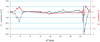 |
Fig. 1. Variation of the horizontal magnetic field component and declination as observed at Tromsø on October 16, 2014. Over 24 h, two substorms were observed. The largest had a negative bay of about 400 nT. |
Generally, the magnetic substorm is considered to be the geomagnetic signature of the cycle of energy loading and unloading in the magnetospheric system as a result of its interaction with the solar wind; the magnetosphere accumulates energy from the solar wind and when a certain energy level is reached, it is released and dissipated through several processes like electric currents, aurora, joule heating, plasmoids, etc. Of special interest here is the substorm electrojet current which is an enhanced westward ionospheric current flow in the midnight sector. The substorm electrojet is concentrated in the region of active aurora and the strength of the current is largely determined by the ionospheric conductance which is increased by particle precipitation when the aurora is active (e.g. Baumjohann & Nakamura 2007).
The ground signature of a magnetic substorm may be described through three phases; the growth, the expansion, and the recovery phase (e.g. McPherron et al. 1973; Baker et al. 1996; Lester 2007). During the expansion phase, the substorm electrojet increases and at the end of this phase, the magnetic perturbation as seen from the ground reaches its maximum.
In general, the ground signatures of magnetic substorms are only a small manifestation of a much larger process on a global magnetospheric scale. During the substorm, a unique substorm current system is set up associated with the disruption of the cross-tail current and magnetic reconnection; instead of flowing across the magnetotail, the current is redirected as Birkeland (also called field-aligned) currents to the ionosphere and an east-west electrojet, and a current wedge is formed between the magnetotail and Earth. Simultaneously, since the cross-tail current disappears, a dipolarization of the tail field lines is experienced, creating a burst of plasma towards the Earth. As more and more of the lobe field lines reconnect, the latitude of the footpoints of the magnetic field lines mapping to the central plasma sheet will increase, and this is seen on the ground during the substorm expansion phase as a northward movement of the auroral and magnetic activity. It is also known that the width of the current wedge increases during a substorm, resulting in an increasing length in the corresponding electrojet in the ionosphere (e.g. Hunsucker & Hargreaves 2003).
Compared to the convectional electrojets, the substorm electrojet current is concentrated around midnight magnetic local time (MLT). The MLT of a specific point at the Earth’s surface is calculated by the angle between the dipole meridional plane, which contains a subsolar point on the Earth’s surface, and the dipole meridional plane, which contains the specific point. A zero angle represents 12 MLT.
The current wedge concept defined by the tail current disruption and short-circuit through the ionosphere via the field-aligned currents (FACs) was first presented by McPherron et al. (1973). A simple version of the current wedge model was used in this study.
1.3. Spatial geomagnetic variations
The Earth’s magnetic field flux density vector B can be described in several ways. In Section 1.1 the spherical coordinates, often used in directional surveying, are mentioned. Additionally, Cartesian or cylinder coordinates can be used. In Cartesian coordinates, the elements X, Y, and Z make up the set of geographic north (X), geographic east (Y), and vertical intensity (Z). The equations for the declination, inclination, and horizontal field are given by the following relationships: (1)
(1)
 (2)
(2)
 (3)
(3)
As described earlier, a critical parameter for the success of drilling operations is the declination. The local declination is mainly given by the Earth’s internal dynamo and the magnetization of the Earth’s crust. However, magnetic disturbances caused by ionospheric currents will produce variations around these values that at times can become too large to be ignored. In most cases, a substorm electrojet will cause a fluctuation in the declination. It is well known that the high latitude currents causing such magnetic disturbances are organized in the reference frame of a geomagnetic coordinate system defined by a dipole (or the first few harmonics of a spherical harmonic representation of the Earth’s magnetic field). This coordinate system does not necessarily relate well to the directions of the magnetic field at ground level (i.e. local D, I, and F). We may therefore assume that the magnetic field disturbance vector has some angle to both the local magnetic meridian as well as the geographic meridian. Furthermore, considering a local magnetic field coordinate system where we are interested in the geomagnetic field variations, we may expect asymmetric effects in the declination. Assuming that a substorm electrojet is flowing parallel to the geomagnetic latitude, the magnetic field from it will be along the local geomagnetic meridian. The geomagnetic meridian is not the same as the magnetic meridian, the difference being that the former is a theoretical direction towards where the Earth’s dipole axis intersects the surface, while the other is the local, measurable horizontal direction of the geomagnetic field. We here define the angle between these meridians and geographic north as dipole declination (DD) and declination (D), respectively. Additionally, we define D′ to be the angle difference between the declination and dipole declination, see Eq. (4).
 (4)
(4)
We acknowledge that the dipole approximation is not necessarily the best way of calculating geomagnetic latitudes of the ionospheric phenomena. Corrected geomagnetic (CGM) coordinate components are proven to reflect the reality better (Laundal & Gjerloev 2014). CGM coordinates are found by tracing the DGRF/IGRF magnetic field line from the specified start point on the ground to the dipole geomagnetic equator and returning along the dipole field line to the ground. The obtained dipole latitude and longitude are assigned as the CGM coordinates to the start point. The International Geomagnetic Reference Field (IGRF) is a mathematical representation of the Earth’s main magnetic field and its secular variation. It is formulated as a spherical harmonic expansion of the scalar potential of the internal magnetic field.
However, for the purpose of this study and owing to its simplicity, we have chosen here to retain the dipole approach since the CGM would not affect the conclusions of the paper, but rather change our D′ somewhat. Qualitatively, as shown later in Figure 4, the sign and magnitude of the fluctuations in the declination (ΔD) are influenced by both the magnitude of the local horizontal magnetic field component and D′. A theory on how the declination is affected by the external magnetic field in the auroral zone was outlined by Edvardsen et al. (2014). Since both the dipole declination and declination vary spatially according to the position on the Earth’s surface, the signature of identical substorms may vary as a function of longitude in certain representations in the local coordinate system (e.g. geographic XYZ, DHZ, or DIF) even though the substorms themselves, in terms of energy, current strength, motion, geomagnetic latitude, etc., are identical.
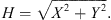
Generally, the Earth’s horizontal magnetic field decreases towards the magnetic poles. In Figure 2, the horizontal magnetic field component, as obtained from the International Geomagnetic Reference Field (IGRF-12) for 2014, is shown for most of the northern hemisphere. Selected locations for observatories and variometers and lines along 67° and 71.5° geomagnetic latitudes (dipole approximation) are also shown.
 |
Fig. 2. The horizontal magnetic field for the northern hemisphere based on IGRF-12 for 2014. The geomagnetic latitudes for 67° and 71.5° are indicated with a dashed and solid line, respectively. |
As seen in the figure, the horizontal component varies considerably as a function of longitude along constant geomagnetic latitudes.
There are also large variations in the declination. In Figure 3, the IGRF-12 values for the declination (D) in 2014 along 67° geomagnetic latitude are plotted together with the dipole declination (DD) and their difference (D′). The largest positive declination is in the western part of Siberia at about 170° geomagnetic longitude while the largest negative declination is at about 30° geomagnetic longitude, in the Labrador Sea. For the dipole declination, the largest negative and positive angles are at about 110° and 250° geomagnetic longitudes, respectively. The largest difference between the declination and the dipole declination is at about 160° geomagnetic longitude in West Siberia.
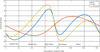 |
Fig. 3. D, DD, and D′ as a function of geomagnetic longitude along 67° geomagnetic latitude. |
An illustration of how the horizontal magnetic field and the declination can be affected by a substorm electrojet is given in Figure 4. The current flows perpendicular to the dipole meridian (HDD), creating a magnetic field disturbance (Hdisturbance) along HDD. Projected onto the nominal (local) horizontal magnetic field (Hnominal), the disturbance field causes a negative deflection of the measured horizontal magnetic field component. The angle between Hnominal and the actually measured horizontal magnetic field (Hmeasured) during the substorm is the deviation of the declination (ΔD), seen here to be in the positive direction.
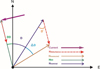 |
Fig. 4. The relationship between the electrojet current and the effect on the horizontal magnetic field and declination. |
To calculate the effect of the electrojet on the horizontal magnetic field and the declination, we made use of a simple trigonometric relationship between the different parameters.
In Table 1, the effect from a substorm causing a negative bay in the horizontal magnetic component (Hdisturbance) of 500 nT is shown for Alaska and West Siberia. Note that for the locations marked with *, the angle D′ is swapped between Alaska and West Siberia in order to illustrate the effect that the magnitude of D′ has on ΔH and ΔD. These values confirm that locations with the smaller nominal horizontal magnetic field are likely to see the larger deviations in declination during geomagnetic disturbances. Furthermore, locations where D′ is small will see the largest negative bays in the horizontal magnetic field and the smallest deflections in the declination.
Estimated deviations in the horizontal magnetic field and the declination at Alaska and West Siberia due to a substorm electrojet.
There are only a few studies where longitudinal variations of magnetic field disturbances have been discussed. Rastogi et al. (2001) analyzed the effect the disturbance field has on the declination at lower latitudes. In his analysis, he also made use of the difference between the declination and dipole declination to explain the variations in the deviation of declination as a function of longitude along constant latitude. He suggested a separate study for higher latitudes, as the current systems are quite different at lower latitudes compared to the auroral zones.
The assumption that the currents in the ionosphere are guided by the geomagnetic dipole field was first described by Birkeland (1908) and implies that currents are directed perpendicular to the geomagnetic meridian. However, it should be noted that during increased geomagnetic activity, the current system in the ionosphere moves equatorward. In such situations, the currents do not necessarily flow parallel to the geomagnetic latitude. However, even though the auroral oval is not always aligned with geomagnetic latitude, this is a good approximation during the period when substorms occur. In a study of the magnitude of fluctuations in the declination for several magnetic observatories in Canada for the years 1976 and 1981, the increased deviations in the declination as one proceeded north, were explained to be solely the result of a decreasing horizontal magnetic field component (Newitt 1991). Brekke et al. (1974) studied incoherent scatter measurements of the E-region conductivities and currents in the auroral zone in Alaska. When comparing the results from the measurements at Chatanika against the geomagnetic variations at the nearby College observatory, they concluded that there was close agreement regarding the variations in the horizontal magnetic field, but not for the variations of the declination. They argued that the observed deviations in the declination were not caused by the auroral electrojet currents alone, but had to be affected by currents parallel to the Earth’s magnetic field too, the FACs. This assumption is in accordance with the description of D (east) component signatures in Kepko et al. (2014), although their focus lies with the magnetic field as measured at lower latitudes than the auroral zone. However, according to Fukushima (1971), the FACs should cause little disturbance at ground level.
In this paper, we aim to examine the effect from the substorm electrojet on magnetic directional surveying. We first present a simple substorm current wedge model which we use to replicate two observed substorms in the northern auroral zone at different longitudes. The two substorms were observed at Tromsø on October 16, 2014 and at Bjørnøya on August 23, 2013. Magnetograms for the two substorms are shown in Figures 1 and 6, respectively. Based on the model, the geomagnetic effects at ground level at different geomagnetic longitudes, but at the same geomagnetic latitude as where the substorms were observed, are analyzed. We are especially interested in the variations in the declination. In order to assess and validate our model results, real geomagnetic data from observatories and variometers within the same area as the model addresses, in the period 2011–2012, are gathered and analyzed statistically. The locations of interest are Siberia, Alaska, Greenland, and the Barents Sea. These are all areas where directional drilling companies drill deviated wells for oil and gas production. Similarities and differences between the collected data and the modelled results are compared and discussed.
2. Substorm current wedge model
We apply a simple line current model to replicate the geomagnetic ground effects of a substorm. The model consists of four current segments that may be interpreted as the equatorial ring current, the substorm electrojet, and the associated Birkeland currents. As illustrated in Figure 5, the coordinate system used for the model has its origin at Earth’s center (we assume a spherical Earth). The XG-axis (subscript G for Global to discern from local xyz discussed earlier) points towards midnight along the Sun-Earth line and the ZG-axis along the magnetic dipole axis. The YG-axis completes the coordinate system by pointing towards dawn. With the model, it is possible to replicate a real magnetic substorm event observed at one location (say Tromsø) and then run an identical substorm at a different location (say Alaska) in order to investigate local differences in its geomagnetic ground signature.
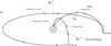 |
Fig. 5. The current wedge model in a Cartesian coordinate frame with the Earth center at the origin. |
The direction of the current in the loop is westward. The equatorial current extends from 22.00 to 02.00 MLT, where 24.00 MLT is along the XG-axis. The Birkeland currents connect the equatorial current in the magnetosphere with the current in the ionosphere at 02.00 h MLT and 22.00 h MLT. Finally, the ionospheric current segment is 4.00 h wide. The substorm is created by allowing currents to flow in the loop as described in the figure during a given time interval, and then tuning the strength and geomagnetic latitude of the ionospheric part of the current as a function of time in order to get the appropriate magnetic signature at a ground location as compared to real data. The magnetic signature is obtained by integration along the current loop for each time step according to the Biot-Savart law: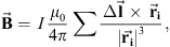 (5)where
  is the resultant magnetic field in teslas, I is the current strength in Amperes, μ0 is the constant for magnetic permeability in vacuum,
  is the vector along a current element, and
  is the vector from
  to the location where the magnetic field is calculated.
  for the equatorial and ionospheric current elements are easily found by polar coordinate trigonometry and the selected step size is 1° in longitude. For the FACs, we make use of a dipole model of the geomagnetic field to calculate the vector elements. The step size was reduced to 0.05° in latitude to avoid too long line segments.
When the geomagnetic latitude of the ionospheric part of the current is altered as a function of time, the length of the FACs and radius of the equatorial ring current will also vary accordingly. The substorms are defined by the time for substorm onset, the times for the end of the expansion and recovery phases, the current strength, and the geomagnetic latitude of the ionospheric current segment. The substorm can be run at any location. By choosing a customized time interval in UT, the Earth’s surface will rotate into the proper location. Any location on the Earth’s surface may be tested with respect to any substorm happening at any time. The calculated magnetic field disturbance vector is rotated into the coordinate system of interest and added to the geomagnetic field as per IGRF-12 for the given time. Finally, the deviations in the horizontal magnetic field and the declination can be calculated.
2.1. Replicating substorms using the current wedge model
The selected substorm events that we would like to reproduce are ordinary substorms, the first (Fig. 1) observed at Tromsø on October 16, 2014 and the second (Fig. 6) observed from Bjørnøya on August 23, 2013. The two magnetograms show the deviations in the horizontal magnetic field component and the declination from quiet level. The quiet level in this study is calculated as per the procedure described in Edvardsen et al. (2013). The substorm current wedge model requires the input data to be represented in a global coordinate system, which may represent a simplification of the magnetosphere and which is fixed with respect to the general direction of the Sun, as illustrated in Figure 5. The Earth is allowed to rotate within this coordinate system. To fit the model output to the actual variations, both the current strength and geomagnetic latitude have been tuned as a function of time. The distance from the Earth surface to the ionosphere is set to 110 km. The assumed current strength is in the order of magnitude from 105 to 106 A. The calculated variations are based on contributions from all the four segments in the current loop.
 |
Fig. 6. Variation of the horizontal magnetic field and the declination as observed from Bjørnøya on August 23, 2013. Most of the day was moderately disturbed with a typical substorm event occurring one hour before magnetic midnight. In 2013, magnetic midnight at Bjørnøya was 21.13 UT. |
2.2. Event 1
The selected substorm event was observed at Bjørnøya on August 23, 2013. This event has the typical substorm signature with a rapid negative bay in the horizontal magnetic component of about 580 nT. The simultaneous deflection in the declination was about 1.9°.
In Figure 7, the actual and modelled magnetic field variations in X, Y, and Z in the geomagnetic coordinate frame for the substorm event at Bjørnøya are shown. The substorm onset was at 19.38 UT (t1) and the maximum modelled variation in X was at 20:14 UT (t2). In total, the substorm lasted for 1.34 h, until 20:59 UT (t3). In the figure, time is in decimal hours. To fit the model to the actual data during the expansion and recovery phases, the strength of the current (I) and the geomagnetic latitude of the current λI are tuned to:
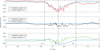 |
Fig. 7. Modelled and actual magnetic field variations in X, Y, and Z at Bjørnøya on August 23, 2013. |
Expansion phase
 (6)
(6)
 (7)
(7)
Recovery phase
 (8)
(8)
 (9)where λO is the geomagnetic latitude for the location of observation.
In the period prior to onset and after the recovery phase, the strength of the current is set to zero.
As can be seen in Figure 7, the parameters chosen reproduce overall shape of the Bjørnøya substorm quite well in the X-component. The reason for the modelled Y-component becoming a flat line throughout the substorm is that the current flows strictly along the geomagnetic latitude and therefore does not produce any significant east-west pointing magnetic field. The variation in the Z-component gives information about the location of the currents compared to the location of observation. A positive variation in Z indicates that the current lies to the south of the point of observation. When the current is in zenith, the variation in Z should be close to zero. During the expansion phase, the general trend for the actual variation is followed, but for the recovery phase the modelled current is tuned to move slower northward than the actual current. This is especially visible in the modelled variation of the Z-component. However, the main parameter of concern here is the X-component. Therefore, we argue that our reproduction of the Bjørnøya substorm is sufficient for the purpose of this work.
2.2.1. Modelled variations in H and D along 71.5° geomagnetic latitude due to substorms identical to Event 1
In Table 2, geographic and geomagnetic information for selected locations along 71.5° geomagnetic latitude at the Kara Sea, the Laptev Sea, Alaska, and the Labrador Sea is listed. As shown in Figures 2 and 3, there are large variations in the geomagnetic field parameters around the globe at high latitudes. For instance, the magnitude of the horizontal magnetic field at the Kara Sea and the Laptev Sea is between 3900 nT and 5200 nT, which is much smaller than at the other locations. In the Kara Sea, D′ is almost 50°, while in Alaska it is only about −1°. IGRF-12 for 2014 is used to calculate the values in the table.
Geomagnetic information for selected areas along 71.5° geomagnetic latitude in 2014. Ggr and Gmag Lat/Long are geographic and geomagnetic latitude/longitude, respectively. H-field is the magnitude of the horizontal magnetic field and Midn MLT is the universal time for magnetic midnight in decimal hours.
In Figures 8 and 9, the variations in the horizontal component and declination caused by the model substorm (Event 1) at different locations are shown. To be able to visually compare the variations along 71.5° geomagnetic latitude, the results from the different locations are time shifted to fit when the actual event was observed at Bjørnøya. The current contribution is from the whole current loop. In Table 3, the effects from each of the current elements are listed.
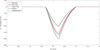 |
Fig. 8. Variations in the horizontal magnetic field at locations along 71.5° geomagnetic latitude due to a modelled substorm that imitates the observed event at Bjørnøya on August 23, 2013. |
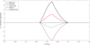 |
Fig. 9. Variations in the declination at locations along 71.5° geomagnetic latitude due to a modelled substorm that imitates the observed event at Bjørnøya on August 23, 2013. |
Maxima in ΔH and ΔD due to the modelled substorm along 71.5° geomagnetic latitude.
The maximum deviation in the horizontal magnetic field along 71.5° geomagnetic latitude occurs in Alaska with −508 nT. The corresponding deviation in the declination here is close to zero. In Alaska, the contribution from the ionospheric current is −565 nT, while the effect from the FACs is 58 nT. The equatorial current has very little effect. For declination, the largest modelled deviation occurs in the Kara Sea area with about 4.9°. The effect from the ionospheric current is about 5.4° and −0.5° from the FACs. When comparing the actual deviations at Bjørnøya against the modelled results, the modelled negative bay in the horizontal component is about 150 nT less than what was observed. The modelled deviation in the declination of 1.9° is very similar to the actual variation of about 1.8°.
2.3. Event 2
In Figure 10, the actual and modelled variations in the geomagnetic coordinate frame of X, Y, and Z for the substorm observed at Tromsø are shown. The time for onset was 21:19 UT (t1) and the expansion phase lasted for 0.7 h and ended at 22:01 UT (t2). After about 2.5 h in total, the substorm was over at 23:49 UT (t3). From onset until the substorm reached maximum deflection in X, the current moved northward at the same time as the strength of the current increased. Equivalent to Eqs. (6)–(9) we define the current strength (I) and the corresponding geomagnetic latitude λI as follows:
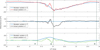 |
Fig. 10. Modelled and actual geomagnetic field variations in X, Y, and Z at Tromsø on October 16, 2014. |
Expansion phase
 (10)
(10)
 (11)
(11)
Recovery phase
 (12)
(12)
 (13)
(13)
As for the substorm at Bjørnøya, the main focus when modelling the substorm observed in Tromsø was to fit the variations in X and make sure that the current moves northward during the expansion phase. The variations in the horizontal magnetic field are mostly dependent on the variations in the X-component. To be able to fit the actual geomagnetic variations in Y, a more advanced model is required where the direction of the current could be adjusted. Regarding Z, the model picks up the main variation in the real data.
2.3.1. Modelled variations in H and D along 77° geomagnetic latitude due to substorms identical to Event 2
In Tromsø, the geomagnetic latitude is about 67° and the locations of comparison lie on the same geomagnetic latitude in the western and eastern parts of Siberia, in the middle part of Alaska, and south in the Labrador Sea, see Figure 2. The magnitude of the horizontal magnetic field in Alaska and the Labrador Sea is between 12,000 nT and 13,000 nT, while in Siberia it is between 6000 nT and 7000 nT, see Table 4. In Tromsø, the nominal H-component in 2014 was about 10,905 nT. The largest D′ is in West Siberia, about 40°, while the counterpart is in Alaska where D′ is almost zero. IGRF-12 for 2014 is used to calculate the values in the table.
Geomagnetic information for selected areas along 67° geomagnetic latitude in 2014.
In Figures 11 and 12, the variations of the horizontal component and declination caused by the modelled Tromsø substorm event are shown. To be able to compare the variations along 67° geomagnetic latitude, the results from the different locations are time shifted to fit when the actual event was observed in Tromsø. The current contribution is from the whole current loop. During the last hour, the curves have a wavy character. This is due to large step length when along the FACs. However, this has no impact on the results we are looking for. In Table 5, the maximum effects from each of the current segments in the current loop are listed.
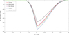 |
Fig. 11. Variations in the horizontal magnetic field at locations along 67° geomagnetic latitude due to a modelled substorm that imitates the observed event at Tromsø on October 16, 2014 |
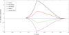 |
Fig. 12. Variations in the declination at locations along 67° geomagnetic latitude due to a modelled substorm that imitates the observed event at Tromsø on October 16, 2014. |
Maxima in ΔH and ΔD due to the modelled substorm along 67° geomagnetic latitude.
Along 67° geomagnetic latitude, the largest negative deviation in the horizontal magnetic field is estimated to occur in Alaska and the Labrador Sea, while the western part of Siberia should see the smallest deflections. The negative variation in Alaska is about 35% larger than what should be seen in West Siberia. However, regarding the fluctuations in ΔD, the two selected areas in Siberia are affected more than anywhere else. A negative bay in the horizontal magnetic field of 241 nT in West Siberia causes a 2.0° deviation in the declination.
In Tromsø the modelled negative deviation in the horizontal magnetic field is 291 nT, which is about 110 nT less than what was actually observed on October 16, 2014. When comparing the modelled and actual variations in the declination, the modelled variations are a bit larger. As in the case of Event 1, the modelled negative deflection of the X-component would have to be smaller to better fit the actual deflection.
3. Analysis of data from observatories and variometers in the northern auroral zone
Geomagnetic data from 13 different locations in the northern auroral zone have been analyzed for the period 2011–2012. The locations are shown in Figure 2 and the corresponding locations are given in Table 6.
Location information for observatories and variometers in the auroral zone.
The selected stations are located in Siberia, Alaska, northern Canada, Greenland, and Norway. Since we are interested in analyzing the geomagnetic effect at ground level caused by substorms, the time span of interest has been restricted to be within ±3 h of magnetic midnight. For a disturbance to be counted as a substorm, the negative bay in the horizontal magnetic field component has to be at least 100 nT (Tanskanen et al. 2005). Together with the variation in the horizontal magnetic field, we have analyzed the substorm effect on declination for the same moment that the maximum deviation in the horizontal magnetic field occurred. It is not certain that this selection method gives us the largest deviations in the declination, but it helps to avoid the inclusion of incidents not caused by substorms.
The number of substorms observed in 2011 and 2012 at the 13 different observatories and variometers are listed in Table 7. The general tendency is that there were more substorms in 2012 than in 2011. In 2012, substorms appeared most frequently in Alaska, especially on the North Slope at Barrow and Deadhorse with more than 280 days with substorms. Siberia generally had the lowest frequency of all areas regarding substorms. There is no clear geophysical explanation as to why there are less observed substorms in Siberia. On the other hand, the geomagnetic datasets for some of the Russian stations were poor, especially Amderma in 2011 and Dikson in 2012. Thus, the results of the analysis for these stations should be taken with care.
The activity level at the selected observatories and variometers in 2011 and 2012. Max/Avg H dev is the maximum and average deviation in the horizontal magnetic field and Max/Avg D dev is the maximum and average deviation in the declination.
In Sections 3.1–3.4 we give a short review of the results in Table 7.
3.1. Barents Sea
Both Bjørnøya and Tromsø are selected due to their location within the Barents Sea. Bjørnøya is an island in the middle of the Barents Sea and Tromsø lies on the Norwegian mainland south of the Barents Sea. At Bjørnøya, about 250 days with substorms were recorded in both 2011 and 2012. In Figure 13, the distribution of the variations in the horizontal magnetic field from the quiet level for 2011 is shown. The maximum, average, and median negative bays in the horizontal magnetic field were 1197 nT, 290 nT, and 242 nT, respectively.
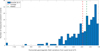 |
Fig. 13. Variation in the horizontal magnetic field for substorms observed at Bjørnøya in 2011. |
In Figure 14, the corresponding variation of the declination from the quiet level at Bjørnøya in 2011 is shown. The maximum deviations range from −2.23° to 4.79° while the average and median deviations were 0.19° and 0.15°.
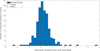 |
Fig. 14. Variation in declination for substorms observed at Bjørnøya in 2011. |
In Tromsø, 197 days with substorms were observed in 2011 and 226 in 2012, see Table 7.
The distribution of the variations in the horizontal magnetic field from the quiet level for 2011 is shown in Figure 15. The maximum negative deviation was 1188 nT, while the average and median deviations were 328 nT and 276 nT, respectively.
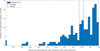 |
Fig. 15. Variation in the horizontal magnetic field for substorms observed at Tromsø in 2011. |
The corresponding deviations in the declination for Tromsø in 2011 are shown in Figure 16. While the maximum deviation for ΔD ranges from −1.51° to 2.71°, the average and median deviations were 0.29° and 0.23°, respectively.
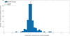 |
Fig. 16. Variation in declination for substorms observed at Tromsø in 2011. |
3.2. Siberia
In the Siberian region, the selected stations are Amderma, Dikson, Tixie, and Pevek. In total, the stations cover about 110° in geographic longitude. For 2012, 212 days with substorms were observed at Tixie, the maximum negative deflection in the horizontal magnetic field component was 1071 nT and the average was 302 nT. The average deviation in the declination at Tixie was −0.48° and the deviations range from −2.87° to 1.84°. To quality check the method of handling the data from the Arctic and Antarctic Research Institute (AARI), the 1991 data from Tixie, found in the Intermagnet database, were analyzed as well. The year 1991 seems to have been slightly more active than 2011 and 2012 with respect to substorms, which is in accordance with the solar cycle. However, the overall results for the variations in the selected geomagnetic components are the same for the two periods and we are therefore confident in our method of handling the AARI data.
3.3. Alaska
The three selected observatory stations in Alaska were College, Barrow, and Deadhorse. Of all the analyzed locations, Barrow and Deadhorse are actually the stations that experienced most substorms, with about 270 days on average each year. At Barrow in 2012, the average negative deflection in the horizontal component was 354 nT and for the declination, the average deflection was 0.22°. College is the location where the largest negative deviation in the horizontal magnetic field for both years was recorded. In 2011, the maximum negative deviation was an impressive 2546 nT and on average for the 155 days of substorms at College, the negative deviation in the horizontal magnetic field was about 392 nT.
3.4. Canada/Greenland
The selected stations in Canada and Greenland are Fort Churchill, Iqaluit, Nuuk, and Ittoqqortoormiit. In 2011, the number of substorms in this area varied from 210 to 231 and in 2012 from 224 to 252. At Fort Churchill in 2011, the average negative deflection in the horizontal component was 266 nT and the maximum negative deflection was 858 nT. Regarding declination at Fort Churchill in 2011, the maximum deflection from the quiet level was −3.14° and 1.27° and on average −0.21°.
4. Discussion and conclusion
The main objective of this paper was to investigate how the geomagnetic variations caused by the external magnetic field vary along constant latitudes in the northern auroral zone. For geomagnetic parameters used in magnetic directional surveying, it is especially interesting to know how the declination is affected by substorm electrojet currents. In order to reproduce the geomagnetic conditions in the northern auroral zone, a substorm current wedge model was developed. In general, the results from the model tell us that the geomagnetic disturbances at ground level, caused by substorm electrojet currents, are longitudinal-dependent in the DIF-coordinate system commonly used in directional surveying.
There are two reasons for this longitudinal dependency:
-
the varying angle difference between the dipole declination and the declination (D′) along constant geomagnetic latitudes;
-
the magnitude of the horizontal magnetic field components varies with geomagnetic longitude along constant geomagnetic latitude.
At locations where the difference between the declination and dipole declination is small, the deviations in the horizontal magnetic field are likely to be large and in declination small. The situation is opposite where the difference between the two angles is large. The impact that the angle difference between the dipole declination and the declination has on the declination during a substorm can be illustrated by looking at the results from Event 1. At Bjørnøya and in Alaska, the nominal H-components are similar: 8922 nT and 9513 nT, respectively. However, the difference between declination and dipole declination is −31.8° at Bjørnøya and 1.2° in Alaska. The results from the substorm model show a negative deviation in the horizontal magnetic field of 422 nT at Bjørnøya and 508 nT in Alaska. Furthermore, we can see that the declination deviation at Bjørnøya is about 1.9° and zero in Alaska. The declination deviation dependency on the horizontal magnetic field can also be illustrated by the results from the modelling of Event 1. At Bjørnøya and the Laptev Sea the differences between the dipole declination and the declination are similar, −31.8° and 28.7°, respectively. However, while the nominal H-component at Bjørnøya is 8922 nT, it is only 3978 nT at the Laptev Sea. The low horizontal magnetic field at the Laptev Sea leads to a modelled deviation in declination of −4.0°, while at Bjørnøya, the estimated deviation in declination is 1.9°. The negative bays in the horizontal magnetic field component are very similar at the two locations, 422 nT at Bjørnøya and 439 nT at the Laptev Sea.
With reference to the results from previous studies at lower latitudes (Rastogi et al. 2001), the results from the substorm current wedge model are as expected as long as the current system is set to be guided by a magnetic field that has a centered dipole configuration. Thus, in the northern auroral zone, the substorm electrojet current should cause the smallest deviations in the declination in Alaska and the largest deviations in Siberia. Intermediate deviations are expected in the Barents Sea region and in Greenland. It is acknowledged that the current wedge model is a simplification of the real and complex substorm system. For instance, the current flow is assumed to follow geomagnetic latitude all the time. On the other hand, we believe that the model is a sufficient tool for this investigation. According to the model, the geomagnetic effect at ground level has the potential to vary largely within the northern auroral zone. Additionally, the substorm current wedge model shows that during a substorm most of the modelled disturbance at ground level is related to the modelled ionospheric current. In our study, the effect from the FACs is only about 15% of the ionospheric current regarding variation in the deviations in the horizontal magnetic field. While the ionospheric current causes a negative bay in the horizontal magnetic field, the FACs contribute in the positive direction.
It is acknowledged that FACs in reality may have a larger effect on the ground magnetic signature than what is obtained with our model. This would most likely be revealed by a more realistic and complex current wedge model, with current sheets included. As discussed by Kepko et al. (2014), FACs cannot be ignored in the analysis of ground magnetometer data, especially at sub-auroral latitudes. However, including magnetic field perturbations from a more complex FAC system would still reveal the longitudinal effects demonstrated in the paper.
The statistical analysis includes geomagnetic data from observatories and variometers from 63.2° to 72.7° geomagnetic latitude in the northern auroral zone. For all of the stations, most substorms are in the range from 100 nT to 250 nT (negative bay in the horizontal component), but quite often the substorms also reach levels of 400 nT–500 nT. In 2011 at Bjørnøya, there were 26 days when the substorms reached this level. When using 100 nT as a limit, substorms were observed in about 60% of the days in both 2011 and 2012. By studying the data by region, e.g. Bjørnøya – Tromsø and Deadhorse – Barrow – College, it is clear that the northernmost locations see most substorms. For the 2011 data, we found 242 substorms at Bjørnøya and 197 substorms at Tromsø. According to Figures 13 and 15, we detected about 30 more substorms at Bjørnøya than at Tromsø in the interval from 100 nT to 200 nT. For 2012, we detected 197 days with substorms at College, while in Barrow and Deadhorse, the numbers are 288 and 284, respectively. These observations are in accordance with the statistical designation “auroral zone”, implying that aurora activity and thereby also substorm activity is higher close to the center of the auroral zone than at locations on the outer edge of the zone.
The overall largest negative bays in the horizontal component are found in Alaska and the smallest in the eastern part of Siberia and in Greenland. The pattern is the same for the average numbers. The difference in the magnitude of the deviations in the horizontal magnetic field relates to the difference between the local declination and dipole declination (D′). However, by studying the stations in Alaska again, it is at College that the largest deviations in the horizontal magnetic field occur. This accounts for both single events and the average numbers. The lower average deviation in the horizontal magnetic field for substorms at Barrow than at College can be explained by a large number of substorms at Barrow that just reach the limit of 100 nT. The reason why the largest deviations for single events are observed in College too, may be related to ground conductivity. For declination, the selected locations in Siberia observed the largest deviations and Alaska the smallest ones.
In general, the results from the statistical analysis of the horizontal magnetic field and the declination variations (Table 7) mostly confirm the results from the current wedge model (Tables 3 and 5). Also the sign of the modelled deflections corresponds well with those found in the statistical analysis. However, for single events, large deviations in declination were also observed in Alaska, although not expected based on the model. This can be explained by asymmetries in the auroral oval during highly disturbed periods. When the auroral oval moves equatorward, the oval will not be parallel to the geomagnetic latitude and thus the current flow will not be directed perpendicular to the dipole meridian. Theoretically, within the ±3 h of magnetic midnight, which is the selected time span for the substorm, the oval should be aligned more or less along the geomagnetic latitude. Outside the chosen time span there are larger chances of having a difference between the direction of the geomagnetic latitude and the electrojet currents. The largest deviations in the declination might therefore not occur during a substorm.
Furthermore, since the selected substorms are solely defined by the deviation of the horizontal magnetic field, the largest deviations in the declination within the selected time interval may not be identified. We have observed that there is sometimes a time shift of the maximum deviations in the horizontal component and the declination. This can be explained by a change in the angle difference between the substorm electrojet current and the geomagnetic latitude throughout the period of a substorm. If, for instance, this angle difference increases after the maximum negative deviation in the horizontal magnetic field has occurred, the deflection in the declination can be larger during the substorm recovery phase than earlier in the substorm cycle.
Limited research on the spatial effect from the external magnetic field on the declination at high latitudes has been conducted. This may be due to the fact that the declination is little used in ionospheric physics. However, for those who are navigating a drilling assembly, it is highly important to know when the currents in the ionosphere are affecting the declination. In some cases, a declination deviation of 1° can cause operational issues if proper procedures on how to handle the external magnetic field effects are missing. Oil companies and directional drilling providers operate globally. Thus, it is crucial for these companies to be aware that there are large regional differences in how the geomagnetic field is affected by substorm electrojet currents. Some areas might need a denser network of variometers and observatories to be able to monitor and correct for external magnetic field variations than others. Especially for offshore locations far from land this can be challenging.
In this paper the main focus has been on how the horizontal magnetic field and the declination are affected by substorms. A separate study of variations in inclination (dip angle in directional drilling terminology) and total field is recommended. One must keep in mind that although the fluctuations in total field and inclination might be within acceptable tolerances, the effect on the declination could be relatively large and lasting, without being detected at the rig site. According to Ekseth et al. (2006) there are no simple ways to directly quality check declination variations. From a directional drilling perspective, a constant declination offset from the quiet level for several hours can have a devastating effect on the wellbore position and the result can be missed geological targets and anti-collision situations (Edvardsen et al. 2014). In such cases, data on the geomagnetic variations at a nearby observatory or variometer should be used to monitor the situation, and if applicable, corrections should be made (Edvardsen et al. 2013).
The following summarizes the main findings of this study:
-
there are large spatial variations in the geomagnetic signature due to the substorm electrojet along constant geomagnetic latitudes;
-
the results from substorm current wedge modelling are verified by statistical analysis of observatory data;
-
the largest deviations in the magnetic field horizontal component due to the substorm electrojet are in the Alaska area, while areas in Siberia have the largest average variations in the declination;
-
directional drilling companies should take into account the longitudinal variations when deciding how to best manage substorm effects on survey measurements.
Acknowledgments
The results presented in this paper rely on data collected at magnetic observatories. We thank the national institutes that support them and INTERMAGNET for promoting high standards of magnetic observatory practice (www.intermagnet.org). We would also like to thank the AARI, DTU, and UiT for giving access to geomagnetic data. Finally, we thank Baker Hughes for the permission to publish this paper.
The editor thanks Martin Connors and an anonymous referee for their assistance in evaluating this paper.
References
- Baker, D.N., T.I. Pulkkinen, V. Angelopoulos, W. Baumjohann, and R.L. McPherron. Neutral line model of substorms: past results and present view. J. Geophys. Res., 101, 12975–13010, 1996. [CrossRef] [Google Scholar]
- Baumjohann, W., and R. Nakamura. Magnetospheric contributions to the terrestrial magnetic field. In: G. Schubert, Editor. Geomagnetism: Treatise on Geophysics, vol. 5, Elsevier, Amsterdam, 77–92, 2007. [CrossRef] [Google Scholar]
- Birkeland, K. The Norwegian Aurora Polaris Expedition 1902–1903, vol. 1, 1st sect., Pitman, London, 1908. [Google Scholar]
- Brekke, A., J.R. Doupnik, and P.M. Banks. Incoherent scatter measurements of E region conductivities and currents in the auroral zone. J. Geophys. Res., 79 (25), 3773–3790, 1974. [CrossRef] [Google Scholar]
- Edvardsen, I., T.L. Hansen, M. Gjertsen, and H. Wilson. Improving the accuracy of directional wellbore surveying in the Norwegian Sea. SPE Drilling and Completion, 28 (2), 158–167, 2013. [CrossRef] [Google Scholar]
- Edvardsen, I., E. Nyrnes, M.G. Johnsen, T.L. Hansen, U.P. Løvhaug, and J. Matzka. Improving the accuracy and reliability of MWD/magnetic-wellbore-directional surveying in the Barents Sea. SPE Drilling and Completion, 29 (2), 215–225, 2014. [CrossRef] [Google Scholar]
- Ekseth, R., T. Torkildsen, A.G. Brooks, J.L. Weston, E. Nyrnes, H.F. Wilson, and K. Kovalenko. The reliability problem related to directional survey data, Paper SPE-133734, Society of Petroleum Engineers, 2006, DOI: 10.2118/103734-MS. [Google Scholar]
- Fukushima, N. Electric current systems for polar substorms and their magnetic effect below and above the ionosphere. Radio Sci., 6 (2), 269–275, 1971. [CrossRef] [Google Scholar]
- Hunsucker, R.D., and J.K. Hargreaves. The high-latitude ionosphere and its effects on radio propagation, Cambridge Univ. Press, Cambridge, UK, 285–322, 2003. [Google Scholar]
- Kepko, L., R.L. McPherron, O. Amm, S. Apatenkov, W. Baumjohann, et al. Substorm Current Wedge Revisited. Space Sci Rev., 190 (1), 1–46, 2014, DOI: 10.1007/s11214-014-0124-9. [CrossRef] [Google Scholar]
- Laundal, K.M., and J.W. Gjerloev. What is the appropriate coordinate system for magnetometer data when analysing ionospheric currents? J. Geophys. Res. [Space Phys.], 119, 8637–8647, 2014. [CrossRef] [Google Scholar]
- Lester, M. Storms and Substorms, Magnetic. In: D. Gubbins, and E. Herrero-Bervera, Editors. Encyclopedia of Geomagnetism, Paleomagnetism, Springer, Dordrecht, The Netherlands, 926–927, 2007. [CrossRef] [Google Scholar]
- Macmillan, S., and S. Grindrod. Confidence limits associated with values of the earth’s magnetic field used for directional drilling. SPE Drilling and Completion, 25 (2), 230–238, 2010. [CrossRef] [Google Scholar]
- McPherron, R.L., C.T. Russell, and M.P. Aubry. Satellite studies of magnetospheric substorms on August 15, 1968: 9. Phenomenological model of substorms. J. Geophys. Res., 78, 3131–3149, 1973. [CrossRef] [Google Scholar]
- Newitt, L.R. The effect of changing magnetic declination on the compass, Energy, Mines, and Resources Canada, Canada Communication Group Pub, Ottawa, Canada, 1991. [CrossRef] [Google Scholar]
- Poedjono, B., S. Maus, and C. Manoj. Effective monitoring of auroral electrojet disturbances to enable accurate wellbore placement in the arctic, Paper OTC-24583, Offshore Technology Conference, 2014, DOI: 10.4043/24583-MS. [Google Scholar]
- Rastogi, R.G., D.E. Winch, and M.E. James. Longitudinal effects in geomagnetic disturbances at mid-latitudes. Earth, Planets and Space, 53 (10), 969–979, 2001. [CrossRef] [Google Scholar]
- Tanskanen, E.I., J.A. Slavin, A.J. Tanskanen, A. Viljanen, T.I. Pulkkinen, H.E.J. Koskinen, A. Pulkkinen, and J. Eastwood. Magnetospheric substorms are strongly modulated by interplanetary high-speed streams. Geophys. Res. Lett., 32, L16104, 2005. [Google Scholar]
- Williamson, H.S., P.A. Gurden, D.J. Kerridge, and G. Shiells. Application of interpolation in-field referencing to remote offshore locations, Paper SPE-49061, Society of Petroleum Engineers, 1998, DOI: 10.2118/49061-MS. [Google Scholar]
Cite this article as: Edvardsen I, Johnsen MG & Løvhaug UP. Effects of substorm electrojet on declination along concurrent geomagnetic latitudes in the northern auroral zone. J. Space Weather Space Clim., 6, A37, 2016, DOI: 10.1051/swsc/2016031.
All Tables
Estimated deviations in the horizontal magnetic field and the declination at Alaska and West Siberia due to a substorm electrojet.
Geomagnetic information for selected areas along 71.5° geomagnetic latitude in 2014. Ggr and Gmag Lat/Long are geographic and geomagnetic latitude/longitude, respectively. H-field is the magnitude of the horizontal magnetic field and Midn MLT is the universal time for magnetic midnight in decimal hours.
Maxima in ΔH and ΔD due to the modelled substorm along 71.5° geomagnetic latitude.
Geomagnetic information for selected areas along 67° geomagnetic latitude in 2014.
Maxima in ΔH and ΔD due to the modelled substorm along 67° geomagnetic latitude.
The activity level at the selected observatories and variometers in 2011 and 2012. Max/Avg H dev is the maximum and average deviation in the horizontal magnetic field and Max/Avg D dev is the maximum and average deviation in the declination.
All Figures
|
Fig. 1. Variation of the horizontal magnetic field component and declination as observed at Tromsø on October 16, 2014. Over 24 h, two substorms were observed. The largest had a negative bay of about 400 nT. |
| In the text | |
|
Fig. 2. The horizontal magnetic field for the northern hemisphere based on IGRF-12 for 2014. The geomagnetic latitudes for 67° and 71.5° are indicated with a dashed and solid line, respectively. |
| In the text | |
|
Fig. 3. D, DD, and D′ as a function of geomagnetic longitude along 67° geomagnetic latitude. |
| In the text | |
|
Fig. 4. The relationship between the electrojet current and the effect on the horizontal magnetic field and declination. |
| In the text | |
|
Fig. 5. The current wedge model in a Cartesian coordinate frame with the Earth center at the origin. |
| In the text | |
|
Fig. 6. Variation of the horizontal magnetic field and the declination as observed from Bjørnøya on August 23, 2013. Most of the day was moderately disturbed with a typical substorm event occurring one hour before magnetic midnight. In 2013, magnetic midnight at Bjørnøya was 21.13 UT. |
| In the text | |
|
Fig. 7. Modelled and actual magnetic field variations in X, Y, and Z at Bjørnøya on August 23, 2013. |
| In the text | |
|
Fig. 8. Variations in the horizontal magnetic field at locations along 71.5° geomagnetic latitude due to a modelled substorm that imitates the observed event at Bjørnøya on August 23, 2013. |
| In the text | |
|
Fig. 9. Variations in the declination at locations along 71.5° geomagnetic latitude due to a modelled substorm that imitates the observed event at Bjørnøya on August 23, 2013. |
| In the text | |
|
Fig. 10. Modelled and actual geomagnetic field variations in X, Y, and Z at Tromsø on October 16, 2014. |
| In the text | |
|
Fig. 11. Variations in the horizontal magnetic field at locations along 67° geomagnetic latitude due to a modelled substorm that imitates the observed event at Tromsø on October 16, 2014 |
| In the text | |
|
Fig. 12. Variations in the declination at locations along 67° geomagnetic latitude due to a modelled substorm that imitates the observed event at Tromsø on October 16, 2014. |
| In the text | |
|
Fig. 13. Variation in the horizontal magnetic field for substorms observed at Bjørnøya in 2011. |
| In the text | |
|
Fig. 14. Variation in declination for substorms observed at Bjørnøya in 2011. |
| In the text | |
|
Fig. 15. Variation in the horizontal magnetic field for substorms observed at Tromsø in 2011. |
| In the text | |
|
Fig. 16. Variation in declination for substorms observed at Tromsø in 2011. |
| In the text | |
Current usage metrics show cumulative count of Article Views (full-text article views including HTML views, PDF and ePub downloads, according to the available data) and Abstracts Views on Vision4Press platform.
Data correspond to usage on the plateform after 2015. The current usage metrics is available 48-96 hours after online publication and is updated daily on week days.
Initial download of the metrics may take a while.