| Issue |
J. Space Weather Space Clim.
Volume 15, 2025
|
|
|---|---|---|
| Article Number | 24 | |
| Number of page(s) | 19 | |
| DOI | https://doi.org/10.1051/swsc/2025021 | |
| Published online | 30 June 2025 | |
Research Article
On the role of source surface height and magnetograms in solar wind forecast accuracy
1
Udaipur Solar Observatory, Physical Research Laboratory, Udaipur 313001, Rajasthan, India
2
Discipline of Physics, Indian Institute of Technology Gandhinagar, Palaj, Gandhinagar 382 355, Gujarat, India
3
Solar-Terrestrial Centre of Excellence – SIDC, Royal Observatory of Belgium, 1180 Brussels, Belgium
4
Institute of Geodynamics of the Romanian Academy, Str. Jean-Louis Calderon 19–23, 020032 Bucharest, Romania
* Corresponding author: This email address is being protected from spambots. You need JavaScript enabled to view it.
Received:
24
October
2024
Accepted:
8
May
2025
Abstract
Many operational space weather forecasting frameworks are based on the Potential Field Source Surface (PFSS) model of the magnetic field. The output of PFSS serves as input in many heliospheric models that provide solar wind velocity predictions at L1. Previous studies in the context of prediction of open magnetic flux observed at L1 have suggested different source surface heights (Rss) for the PFSS model at different phases of the solar cycle (SC). We investigate the effects and necessity of optimizing the Rss in the PFSS model in the context of its use in the popular Wang-Sheeley-Arge (WSA) model for solar wind velocity prediction. We used Heliospheric Upwind Extrapolation (HUX) to extrapolate solar wind velocity in the heliosphere. We performed a study of 16 Carrington Rotations (CR) at different phases of the SC24 and SC25, using different types of magnetograms and WSA model parameters. We combine the coronal models (PFSS+WSA) with the heliospheric model (HUX) to predict solar wind velocity at L1 in our framework, i.e., PFSS+WSA+HUX. Our study suggests that using a higher Rss (3.0 R⊙) compared to the conventional Rss (2.5 R⊙) near the solar minimum, results in an improvement in the average Pearson’s correlation coefficient (cc) from 0.61 to 0.75 between the observed and modeled values of solar wind velocity profile at L1. We found that the performance of the framework improved by using zero-point corrected (ZPC) maps in comparison to the standard (STD) Carrington maps from GONG, as demonstrated by an increase in the correlation coefficient from 0.31 to 0.51. We also found that the improved performance of the framework for ZPC maps as compared to the STD full Carrington maps, can be attributed to its capability to capture the global magnetic field. This was further confirmed by comparing the extrapolated global magnetic field structures with the large-scale corona observed in the extended field of view of the PROBA2/SWAP images. Our work is a first step in the direction of improving the WSA model and points out the potential ways to enhance the PFSS+WSA framework of solar wind forecasting at L1.
Key words: Solar wind / Potential field source surface / Magnetograms / Heliosphere / Wang-Sheeley-Arge
© S. Kumar et al., Published by EDP Sciences 2025
 This is an Open Access article distributed under the terms of the Creative Commons Attribution License (https://creativecommons.org/licenses/by/4.0), which permits unrestricted use, distribution, and reproduction in any medium, provided the original work is properly cited.
1 Introduction
Many of the semi-empirical physics-based operational space weather forecasting frameworks, such as Wang-Sheeley-Arge (WSA)-ENLIL (Arge & Pizzo, 2000; Odstrcil et al., 2004), European heliospheric forecasting information asset (EUHFORIA; Pomoell & Poedts, 2018), and Space Weather Adaptive Simulation Framework for Solar Wind (SWASTi; Mayank et al., 2022), are based on magnetic field extrapolation models. These frameworks combine the coronal magnetic field and heliospheric models to forecast the solar wind properties at L1. Generally, the Potential Field Source Surface (PFSS; Schatten et al., 1969) extrapolation model, which provides an overall magnetic field environment, is used as an input in empirical solar wind models. PFSS is the first-order and lowest-energy approximation of the magnetic field of the Sun as compared to other computationally expensive and more advanced magnetic field models like Nonlinear Force-Free Field (NLFFF; Wiegelmann, 2004; He et al., 2011) and Linear Force-Free Field (LFFF; Alissandrakis, 1981) models. Further, there is a class of models providing full 3D MHD treatment to the coronal domain, such as Alfvén Wave Solar Model (AWSoM; van der Holst et al., 2014) and data-driven COolfluid COroNa UnsTructured (COCONUT; Perri et al., 2022) model. The quick computation time makes PFSS a suitable choice for use in operational space weather forecasting frameworks. The magnetic field from PFSS is used as an input in empirical solar wind models like Wang-Sheeley (WS; Wang & Sheeley, 1990), Distance from Coronal Hole Boundary (DCHB; Riley et al., 2001), and the Wang-Sheeley-Arge (WSA; Arge et al., 2003).
The main PFSS parameter is the height of the source surface, and it is crucial for the extrapolation of the field above the photosphere. Kruse et al. (2020) also investigated the effects of changing the shape of the source surface from a sphere to an ellipsoid. The source surface height (Rss) in the PFSS model defines the upper boundary where the magnetic field lines are open and radial in the heliosphere. This parameter has two physical effects. First, Rss controls the open flux in the heliosphere. Second, this height also changes the overall magnetic field structure and connectivity of the Sun to the Earth.
Due to the change in the state of the solar magnetic field structure with the phase of the solar cycle (SC), the source surface height is expected to change accordingly (Schatten et al., 1969). This change in source surface height can be studied through various observable outputs provided by the PFSS model. These outputs include the open flux at L1, which can be compared with interplanetary magnetic field (IMF) data from in situ observations. The PFSS model can also be used to estimate the photospheric footpoints of the open field lines. These footpoints can then be compared to coronal hole (CH) locations in different wavelengths in synoptic images (Lowder et al., 2017).
Recently, Meyer et al. (2020) used a global non-potential coronal magnetic field model to estimate the global magnetic field structure, which was compared with the features observed in Sun Watcher using Active Pixel System Detector and Image Processing (SWAP; Berghmans et al., 2006) images, onboard Project for On-Board Autonomy 2 (PROBA2; Santandrea et al., 2013) to study the short-term evolution of the solar magnetic field over the maximum of the SC24. However, their global coronal magnetic field model is computationally expensive to apply over the entire SC compared to PFSS.
Several attempts have been made to assess the change of source surface height in the PFSS model with the phase of the SC. For example, using photospheric magnetic synoptic maps from Mount Wilson Observatory (MWO), Lee et al. (2011) reported that the Rss of 1.9 R⊙ and 1.8 R⊙ produced the best results for the modeled IMF at L1 for the minimum periods of SC22 and SC23, respectively. Moreover, they found that 1.5 R⊙ and 1.8 R⊙ provided the best IMF during the SC23 maximum and minimum, respectively, in Figure 6 of Lee et al. (2011). A study by Arden et al. (2014) using synoptic maps from Solar and Heliospheric Observatory’s Michelson Doppler Imager (SOHO/MDI; Scherrer et al., 1995) and Solar Dynamics Observatory’s Helioseismic and Magnetic Imager (SDO/HMI; Scherrer et al., 2012) showed that raising Rss by 15–30% (2.88–3.28 R⊙) during the SC 23 minimum as compared to the conventional Rss (2.5 R⊙) better reproduces the observed open flux at L1. Therefore, both studies using different magnetic maps reported an increase in the source surface height during the SC minimum compared to the maximum. A study by Nikolić (2019) suggested a lower source surface height (1.5–2.0 R⊙) as compared to the conventional source surface height during the maximum phase of the SC24. The above-mentioned three studies disagree with each other in terms of the best absolute values of the source surface heights. However, they agree in terms of the relative changes in the best source surface heights with the phase of the SC, i.e., to use a higher source surface height during solar minimum as compared to solar maximum. A recent study by Huang et al. (2024) showed that slightly lower and higher values compared to the conventional value of Rss = 2.5 R⊙, at SC minimum and maximum, respectively, provide better values of unsigned open flux at L1. Similarly, Badman et al. (2020), based on the Parker Solar Probe (PSP; Fox et al., 2016) IMF observations during the October–November 2018 period, showed that reduced source surface height improves accuracy of the predicted IMF on specific days (2018-10-20 and 2018-10-29) at PSP located at 0.5 AU. It is important to mention that the two studies focused on distinct selective time periods, whereas the findings of Lee et al. (2011) and Nikolić (2019) are based on long-term analysis for Rss in a different context.
One of the important aspects of Rss optimization is in the context of the use of PFSS in solar wind velocity prediction models at L1. Forecasting solar wind throughout the heliosphere requires accurate magnetic-field extrapolation from the photosphere to the outer boundaries of the coronal domain and, after that, tracing of the magnetic field lines in the coronal domain. Using the properties of the traced field lines in the coronal domain, empirical solar wind models, like WSA, provide the solar wind velocity profile at the outer boundary of the coronal domain. Further, to predict solar wind velocity at L1, extrapolation of the velocity in the heliosphere is required using sophisticated MHD codes or simple 1D ballistic extrapolation. Riley & Lionello (2011) proposed a simple model called Heliospheric Upwind eXtrapolation (HUX), which is computationally cheaper than sophisticated MHD codes and incorporates more physics than a simple 1D ballistic extrapolation, and can be used for more reliable solar wind velocity estimates at L1.
Currently, the community uses a constant source surface radius (2.5 R⊙) for PFSS in the WSA model with the standard synoptic magnetic maps from the Global Oscillation Network Group (GONG) network (Riley et al., 2015; Reiss et al., 2019; Kumar et al., 2020; Narechania et al., 2021; Kumar & Srivastava, 2022; Mayank et al., 2022). As reported by Lee et al. (2011), a small change in the Rss can change the degree of agreement between the modeled and observed values of IMF at L1. In an earlier study, we have shown that the performance of solar wind velocity forecasting models decreased significantly during the deep solar minimum of SC23 (Kumar & Srivastava, 2022). This study considered a fixed source surface radius in the PFSS model. Since previous studies suggested that Rss changes with the phase of the SC, therefore, one of the reasons for the decreased performance of the framework in our study can also be attributed to the usage of a fixed source surface radius (Rss), i.e., 2.5 R⊙.
The output of the WSA model changes with the source surface radius because changing Rss affects the overall simulated magnetic field structure of the Sun, leading to changes in the connectivity of sub-Earth field lines. Thus, there is a clear need to optimize Rss and the WSA parameters for solar wind forecasting at L1.
In this work, we optimize Rss in the PFSS model with the phase of the SC to be used in the WSA model. We evaluated the performance of the solar wind velocity prediction framework (PFSS+WSA+HUX) at L1 using different Rss, for 16 Carrington Rotations (CRs) selected at different phases of SC24 and SC25 as shown in Figure 1. Section 2 describes the data selected and the methodology, consisting of the extrapolation method for the magnetic field and the estimation of solar wind velocity in the heliosphere. Section 2.1 provides details about the models used in the framework and the parametric space for the source surface radius in the WSA model. In Section 3, we discuss the main results and their interpretations. Finally, in Section 4, we present our main conclusions.
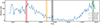 |
Figure 1 Monthly sunspot numbers (blue line) plotted with time, indicating different phases of solar activity cycle 24 and 25. Vertical lines mark the CRs selected for analysis at different phases of the SC. |
2 Data and methodology
We consider the space between the Sun and the Lagrangian point L1 as two distinct regions. The first region extends from the photosphere to the source surface. The second region extends from the source surface to the L1 point. We use a combination of different models, PFSS+WSA+HUX, in the framework to estimate the solar wind velocity at L1.
The input magnetograms for PFSS specify the inner boundary conditions for the magnetic field at the solar surface. Our approach is solely based on the magnetic field extrapolation, which is sensitive to the magnetic field inputs provided to the model. Therefore, we explore the use of the three different types of magnetic field maps, taken from the Global Oscillation Network Group (GONG)1. Out of the three types of magnetic maps, two are full (CR) synoptic maps commonly used by the community: standard magnetic (“mrmqs” in the GONG file name) and integral zero-point corrected (ZPC) maps (“mrnqs” in the GONG file name). Due to differences in location and observing conditions between the various sites of the GONG network, strong background variations were observed in the standard magnetic GONG maps (Hill, 2018). These so-called zero point errors reached amplitudes of the order of 10 G, but were reduced to 1G with an automated comparison between sites and day-to-day variations, resulting in the ZPC map. We also used the hourly updated ZPC (HU ZPC) synoptic maps (“mrzqs” in the GONG file name) at an interval of 5 h. The HU ZPC maps were chosen to provide an updated representation of the magnetic field of the Sun.
Monthly sunspot data were obtained from the SILSO website2 to identify different phases of the SC and select different time periods of study. Further, we used the in-situ observations of hourly averaged solar wind velocity recorded at L1 in the OMNI database3 to compare with modeled solar wind velocity profiles at L1.
Since we aim to optimize the source surface height at different phases of the SC, we therefore selected CRs at different phases of the SC. We selected in total 16 CRs: four consecutive CRs at the maximum phase of the SC24 (CR2143 – CR2146, October 2013–January 2014), 8 CRs in the declining and minimum phase of the SC24 (CR2182 – CR2185, September–December 2016 and CR2193 – CR2196, July–October 2017), and 4 CRs at the maximum phase of the SC25 (CR2272–CR2275, January–September 2023), as shown by red, yellow, black, and green vertical lines, respectively, in Figure 1.
Predicting solar wind velocity at the L1 point for these 16 CRs and selecting the best Rss among three choices, i.e., 2.0 R⊙, 2.5 R⊙, and 3.0 R⊙, for each type of input magnetic map in the framework involves the following steps:
Calculate the coronal magnetic field in the coronal domain up to Rss, using the PFSS extrapolation with a Python module pfsspy (Stansby et al., 2020). We use three different values of Rss (2.0 R⊙, 2.5 R⊙, and 3.0 R⊙) for each of the three different types of input synoptic magnetic maps.
Trace the magnetic field lines starting from the photosphere to create a map of open and closed field lines with 1° resolution (Sect. 2.2).
Trace the sub-Earth field lines from Rss to the photosphere (Sect. 2.2).
Utilize the WSA empirical velocity relation to estimate solar wind velocity profile at Rss, based on the magnetic field line properties, using:
default WSA parameters;
a parametric space of WSA parameters. Using parametric space involves a range of values of WSA parameters to conclude independently of the choice of parameters (Sect. 2.3).
Extrapolate velocity estimates from the outer boundary of the coronal domain (Rss) up to the L1 point using the HUX extrapolation (heliospheric domain) (Sect. 2.1).
Apply the first three steps for each value of Rss, with default WSA parameters and for parametric space (Table 1) for each type of magnetic map, and calculate the performance matrix defined by Pearson’s correlation coefficient between the modeled and observed solar wind velocity values at L1 to find the best Rss (Sect. 2.3).
Parametric space used for WSA model.
Finally, in order to compare the quality of the extrapolation of PFSS close to the Sun using different synoptic magnetic maps as inputs, we used observations from the Sun Watcher using Active Pixel System Detector and Image Processing instrument, which is an EUV imager with a passband centered at 174 Å onboard Project for Onboard Autonomy 2 mission (Berghmans et al., 2006; Santandrea et al., 2013; Halain et al., 2013; Seaton et al., 2013; West et al., 2022). SWAP images the solar corona at a cadence of 110 s. This passband provides an excellent opportunity to observe features like active regions (ARs), streamers, and coronal fans that dominate the large-scale structure of the lower corona. Even though 174 Å is not an ideal wavelength for observing coronal holes and filaments, they are still visible and traceable in SWAP images. All these features have a direct connection with the overall magnetic field configuration of the corona. SWAP has a wide field of view (FOV) spanning 54′, and using the off-pointing capability of PROBA2, the SWAP FOV can be shifted in any direction in order to track coronal features of interest up to more than 2 R⊙. This extended FOV is large enough to observe the lower corona and is well within the domain of PFSS extrapolation.
We used observations from special observational campaigns to extend the FOV of SWAP by putting the Sun at the corner of the FOV and recording 30-second exposure images in 174 Å every minute. Finally, we created a single mosaic image by stacking these off-limb images for one hour by keeping the Sun at the center of the mosaic to combine the signal (median of the photon count). This resulted in better visibility of limb features compared to the normal image of the SWAP at larger heights due to increased signal in the overlapped FOV of individual images in the stack. Specifically, we used mosaics reconstructed from the special campaigns on 20 August 2017 and 7 August 2023. These mosaics result in a larger FOV (up to 2.5 R⊙ on the side and 3.0 R⊙ on the corners) as compared to a standard SWAP image centered at the Sun (up to 1.7 R⊙ on the side and 2.5 R⊙ on the corners). It is important to mention here that the mosaics obtained using this approach are suitable only for the study of stable and long-lived features in the corona because short-lived features are smeared out over the time span of an hour. However, this method is suitable for the comparison of SWAP images with the PFSS extrapolated global magnetic field structure.
To be noted that CRs 2194 and 2274 and their neighbouring CRs during the maximum phase of SC25 and the declining phase of SC24 were mainly chosen for this study to include the period for which the extended FOV PROBA2/SWAP mosaic images were available. This was required to compare the SWAP images with the PFSS extrapolation around the time of the optimization of the WSA model. Moreover, we selected a relatively stable period during the SC24 maximum, when the HUX model is expected to give better results since it is essentially a steady-state extrapolation model.
The following sections explain the empirical formulation for solar wind velocity, the extrapolation technique in the heliosphere, and the parametric space of the WSA model, as well as methods of assessment of the framework.
2.1 Coronal and heliospheric model
Using the PFSS model, we first extrapolate the magnetic field in the coronal domain, then we trace the magnetic field lines from the photosphere to the Rss. It provides a map of the footpoints of open and closed field lines on the Sun. We also traced the sub-Earth field lines (field lines corresponding to the sub-Earth points in the CR frame of reference) from Rss to the photosphere to calculate parameters of the field lines. The particular form of the WSA model equation used in our framework is given by Riley et al. (2015):
 (1)
(1)
Here, the expansion factor (fs) is the magnetic flux ratio for a field line between the photosphere and Rss, and θb is the angular distance of field line footpoints to the nearest CH boundary, vslow and vfast represent the tunable slowest and fastest solar wind velocities at Rss, with default values set as vslow = 250 km/s and vfast = 750 km/s. Parameters α, β, γ, δ, and w are tunable in the model, with default values set as α = 1.5/9, β = 1.0, γ = 1.0, δ = 1.5 and w = 0.01. These values provide overall optimal results for the time periods analyzed, but they are not necessarily the best values for each CR. The use of the parametric space, i.e., the range of the values for each parameter, makes the final results independent of the choice of the WSA parameters (Sect. 2.3).
Comparing the estimated solar wind velocity with that observed by spacecraft at the L1 point requires connecting solar wind velocity obtained from the WSA model with heliospheric velocity extrapolation models. As mentioned earlier, we use the HUX Riley & Lionello (2011) model. HUX is better than the simple 1D ballistic approximation as it incorporates a stream interaction term in the momentum equation, and it is faster than the full MHD approximation, providing very similar results for solar wind velocity at L1 when compared with MHD results (cc = 0.98) as reported by Riley & Lionello (2011). We used HUX extrapolation with 0.55° (≈1 h in CR time period) resolution to compare with hourly average data at L1. The same resolution is also used for tracing the sub-Earth field lines from Rss to the solar surface.
After the extrapolation of the solar wind velocity profile from Rss at L1 using HUX, we compared the values of estimated solar wind velocity with the observed values at L1. We use Pearson’s Correlation Coefficient (cc) to assess the performance of the framework, which has values between [−1, 1], with 1 indicating a direct linear correlation and −1 an inverse correlation. Since we aim to find a modeled solar wind profile that closely matches the observed profile, for our study, a cc value close to 1 is desirable, and lower values of cc, including negative ones, may be considered as poor correlation. We also calculate other metrics, such as Mean Absolute Percentage Error (MAPE) and Standard Deviation (SD), as discussed in Kumar & Srivastava (2022). For a set of N modeled values (mi) and a corresponding observed values (oi), the MAPE can be given by
 (2)
(2)
For the sake of simplicity, the assessment of the performance of the framework in this work is solely based on the maximum values of cc. However, we will discuss the results based on the values of MAPE and SD in the specific case of SC25 maximum phase (see Sect. 3).
2.2 Field line tracing approaches corresponding to different types of GONG maps
As mentioned earlier, we have used three types of magnetic maps. Two out of the three maps are full CR maps, i.e., ZPC and standard maps (STD), giving us an idea about the overall magnetic field over 27.27 days (Carrington Rotation time period). We also used hourly updated zero point corrected (HU ZPC) maps to provide a more updated version of the magnetic field. Therefore, we have two types of magnetic maps, i.e., full CR maps and hourly updated synoptic maps. Further, we use two different extrapolation schemes for these three types of maps while tracing the sub-Earth field lines.
For both full (ZPC and STD) and HU ZPC synoptic maps obtained from the GONG network, we traced field lines all over the photosphere to create a map of footpoints of open (field lines reaching at Rss) and closed field lines (field lines closing back to the photosphere) used for the calculation of θb.
In the case of full CR maps, we created a 360° (corresponding to full CR) input for the HUX model and then calculated fs and θb (parameters for the WSA model) for all sub-Earth field lines from Carrington longitude 0° to 360° by tracing all sub-Earth field lines from Rss to the photosphere from a single CR map.
Each HU ZPC map corresponds to a specific central Carrington longitude for a given Carrington rotation based on the observation time. It also represents a full rotation with updated observations for the next 60° of the upcoming Carrington longitude, as described on the GONG website4. Further, tracing the sub-Earth field lines for 129 HU ZPC maps selected at the interval of 5 h, for a CR involves the following steps:
For a given HU map of a given time, trace the field lines all over the photosphere with 1° resolution, from the photosphere to Rss to create a map of the footpoints of open and closed field lines at the photosphere. This step is vital for the calculation of θb using an updated magnetic map.
Trace the sub-Earth field lines, from Rss to the photosphere (to calculate fs and θb), corresponding to the 5-hr time gap between the two maps. It corresponds to tracing the field line for the Carrington longitudinal gap of ≈2.74°. Therefore, each HU map is used to create an HUX input for ≈2.74° only.
Repeating the above two steps for all the HU maps for a given CR to create a full 360° input for the HUX model.
This approach provides an updated view of the coronal magnetic field than a single full CR map. Detailed explanations about the tracing of field lines can be found in Reiss et al. (2019). Figure 2 shows the flowchart of the overall methodology adopted for the two kinds of magnetic maps and the two approaches used in this work.
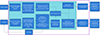 |
Figure 2 Flow chart of the methodology adopted in this work to find optimal Rss. Steps mentioned in the magenta colour box are repeated for all three choices of Rss, i.e., 2.0 R⊙, 2.5 R⊙, and 3.0 R⊙. |
2.3 Optimization of the source surface height using two approaches
We applied two different approaches for each type of magnetic map used as input (STD, ZPC, and HU ZPC) to find the best Rss for each CR. In our first approach, following Kumar & Srivastava (2022), we used default parameters (vslow = 250 km/s, vfast = 750 km/s, α = 1.5/9, β = 1.0, w = 0.01, γ = 1.0, and δ = 1.5) in the WSA model for every CR. For each of the three values of Rss (2.0 R⊙, 2.5 R⊙, and 3.0 R⊙), the velocity profile at the outer boundary of the coronal domain was obtained. This was provided as input to the HUX model to give us velocity output at L1. We then compared these values with the observed solar wind profile at L1 from the OMNI database and estimated Pearson’s correlation coefficient (cc). The Rss corresponding to the maximum cc was selected as the best performing for each CR.
In the second approach, we use various combinations of WSA parameters with values around the default values mentioned in Table 1 to estimate the maximum value of the cc for each Rss. This involves creating 16,200 velocity profiles using an automated Python code at each source surface height, which corresponds to a combination in the parametric space covering Vslow, Vfast, α, β, γ, δ, and w (16,200 = 3 × 5 × 6 × 4 × 5 × 3 × 3, see Table 1). For a given Rss, it further involves extrapolation of each velocity profile (corresponding to each parametric combination) up to L1 using HUX, and calculating cc for each extrapolated velocity profile with the observed in-situ solar wind profile at L1. Thereafter, Rss corresponding to the highest cc (among the three values of Rss) is selected as the best Rss for every CR. Therefore, using parametric space enables us to estimate the best performing Rss independent of the choice of WSA parameters.
3 Results and discussion
We used two approaches to estimate the optimized value of Rss for 16 CRs selected at three different phases, i.e., 8 CRs at the minimum of SC24 and 4 CRs each at the maximum of SC24 and SC25, as shown in Figure 1. In our first approach, we used default WSA parameters, and in the second, we used the parametric space for each Rss (as explained in Sect. 2.3). For both approaches, we also used three different magnetic maps as input (as mentioned in Sect. 2). Therefore, we have a total of 24 (4 × 2 × 3), 48 (8 × 2 × 3), and 24 (4 × 2 × 3) different instances (no. of CRs × no. of methods × no. of maps) to evaluate the best performing Rss at each phase of the SC24 maximum, SC24 declining/minimum phase, and SC25 maximum, respectively. In Section 3.1, we discuss our results obtained from the two approaches and the statistical results based on the above-mentioned different instances. In Section 3.2, we discuss how different values of Rss affect the modeled solar wind profile at L1, specifically for CR2143 and CR2183. In Section 3.3, we compare the extrapolated magnetic field structures using different magnetic maps with the observed large-scale structures in PROBA2/SWAP images with extended FOV.
3.1 Source surface height optimization at different phases of SC24 and SC25
Figure 3 depicts the performance of the framework in terms of Pearson’s cc obtained between the observed and modeled values of solar wind velocity at L1 for different CRs with different Rss based on default WSA parameters, for all three kinds of maps used. In this figure, blue, orange, and green dots represent the performance of the framework (cc), for Rss of 2.0 R⊙, 2.5 R⊙, and 3.0 R⊙, respectively, for each CR. Horizontal dashed lines show the average performance in the respective phase for each Rss and all CRs. The annotated value shows the average value of cc for each input map and SC phase for all three Rss (dashed lines). From Figure 3, we can clearly draw the following conclusions:
The overall performance during the declining phase of SC24 (ccavg = 0.45 averaged over all Rss, CRs, and maps) is better compared to the performance during the maximum of SC24 (ccavg = 0.38).
The framework performed best for Rss = 3.0 R⊙ (green dots) in the declining/minimum phase of SC24 for most of the cases (17/24 combined for all the maps). The orange dashed lines show the average cc for Rss = 2.5 R⊙, which is estimated to be 0.61 for ZPC maps and 0.52 for HU ZPC maps. The green dashed lines show the average cc for Rss = 3.0 R⊙, which is estimated to be 0.75 for ZPC maps and 0.61 for HU ZPC maps. These values show clear improvement using Rss = 3.0 R⊙ in comparison to Rss = 2.5 R⊙, for both the maps. In contrast, the STD maps do not show a significant improvement in performance when using Rss = 3.0 R⊙ as compared to Rss = 2.5 R⊙.
During the SC24 maximum phase, the average performance of the framework for all 4 CRs is the best for either Rss = 2.5 R⊙ or Rss = 2.0 R⊙ for all three types of magnetic maps (blue and orange dashed lines). It is also important to note that, in none of the maps, the average performance reaches its highest value at Rss = 3.0 R⊙.
The overall performance using full ZPC maps is found to be better than standard CR maps at the SC24 maximum and declining phases, and for all three values of Rss. This is highlighted by the increase in the average cc during the minimum phase of the SC24 from 0.31 (for STD maps) to 0.51 (for ZPC maps), and from 0.22 to 0.47 during the maximum phase of the SC24. We also note that the performance using hourly updated ZPC and full CR ZPC maps is similar.
Average cc was consistently negative (ccavg = −0.11) during the SC25 maximum when default WSA parameters were used with all magnetic maps, indicating the poor performance of the framework for this time period.
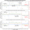 |
Figure 3 The performance of the framework (cc) for different CRs with different Rss based on default WSA parameters. For SC24, refer to the left y-axis, whereas for SC25 maximum, refer to the right y-axis in red. The top panel shows the result using standard Carrington maps (STD), the middle panel is for the zero-point corrected Carrington maps (ZPC), and the bottom panel is for hourly updated zero-point corrected maps (HU ZPC). Blue, orange, and green dots represent the performance of the framework, i.e., cc, for Rss of 2.0 R⊙, 2.5 R⊙, and 3.0 R⊙, respectively. Horizontal dashed lines show the average performance in the respective phase for each Rss and all CRs. The annotated value shows the average value of cc for each input map and SC phase for all three Rss (dashed lines). |
Figure 4 displays the performance of the framework for different CRs with different Rss based on optimized cc, by using the parametric space of WSA parameters. Each dot represents the highest cc in the parametric space for every Rss.
It is important to note that during SC25 maximum, cc optimization showed unrealistic improvement in cc (Fig. 4) as compared to other phases, i.e., average cc increased from negative values to significant positive values for all the maps. In such a case, it becomes important to check the values of the other metrics as well to examine whether this improvement represents a better match or not. Interestingly, we found that other metrics, such as the average MAPE, increased significantly for the SC25 maximum. In this time period, average MAPE increased from approximately 20–22% (for all maps), to 58%, 114%, and 39% for STD, ZPC, and HU ZPC maps, respectively (Figs. A1 and A2 in Appendix). Physically, MAPE represents the mean of the absolute percentage difference between each point in the time series of the modeled and observed solar wind velocity profile for a given CR, and it should be lower for a better match. Similarly, a considerable increase in SD also occurred during the maximum phase of SC25 in ZPC maps, rising from 93 km/s to 160 km/s as a result of cc optimization. Therefore, despite the increase in average cc during the SC25 maximum phase through optimization of WSA parameters, it does not represent an improved match in the solar wind velocity at L1 because of the increase in errors. On the other hand, during the maximum and declining phases of SC24, the default WSA parameters yielded better performance compared to the SC25 maximum, even without optimization. Furthermore, optimization of the cc parameter during the SC24 declining and maximum phase did not result in a significant increase (≤40%) in MAPE and SD, as compared to the increase in the MAPE (up to 200%) and SD (up to 70%) in the case of the SC25 maximum.
Although we used the parametric space (second approach) to obtain the best Rss, independent of WSA parameters, however, during the declining phase of the SC24, both approaches led to Rss = 3.0 R⊙ as the best performing Rss. Moreover, during the SC24 maximum, either Rss = 2.0 R⊙ or 2.5 R⊙ outperformed Rss = 3.0 R⊙ for our second approach by using HU ZPC and STD maps.
The trend of the best-performing source surface heights at each phase, as mentioned earlier, remains the same even after using parametric space for three types of input magnetic maps. Therefore, the improvement in performance on using the higher values of Rss in every CR is independent of the choice of the different maps and the WSA parameters. We can make the following inferences from Figure 4:
Optimization of WSA parameters significantly increased the cc for every CR and at every Rss (when compared with Fig. 3).
The overall trend of the performance in the declining/minimum phase of the SC24 remains the same, as it was for the default WSA parameters approach, for different Rss, i.e., the best performing Rss in most cases (18/24 combined for all the maps) is 3.0 R⊙ (green dots). The average cc values for Rss = 2.5 R⊙ (orange dashed lines) corresponding to the STD, ZPC, and HU ZPC maps have been determined to be 0.49, 0.61, and 0.64, respectively. The average cc values for Rss = 3.0 R⊙ (green dashed lines) corresponding to STD, ZPC, and HU ZPC maps have been estimated as 0.55, 0.72, and 0.72, respectively. These values demonstrate clear improvement in framework performance for all the three maps when using Rss = 3.0 R⊙ as compared to Rss = 2.5 R⊙.
During the SC24 maximum phase, the average performance of the framework is the best for either Rss = 2.5 R⊙ or 2.0 R⊙ for all maps (orange and blue dashed lines). The relative increase in average performance is not as significant as it is during the minimum phase.
As mentioned at the beginning of this section, we have a total of 24, 48, and 24 different instances to evaluate the best performing Rss at the SC24 maximum, SC24 declining/minimum phase, and SC25 maximum, respectively. Figure 5 shows a histogram indicating when different values of Rss were found to be the best choice at different phases of SC24 and SC25 (please note that CR2182 – CR2185 and CR2193 – CR2196 are in SC24 declining phase). An important inference from this bar graph is that Rss = 3.0 R⊙ is the most suitable choice for the maximum number of CRs (35/48) during the declining/minimum phase (middle panel Fig. 5).
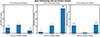 |
Figure 5 Number of cases for different Rss in the best-performing scenario during the selected phase of the SC. Note, as explained in Section 3, the framework performed poorly for the SC25 maximum phase. Therefore, the results from the right panel are inconclusive. |
Moreover, it may be safe to mention that the number of cases of best performance at lower Rss is larger during the maximum of SC24 ((8+12)/24, Fig. 5), as compared to SC24 minimum ((11+2)/48, Fig. 5) leading to an average best performance at Rss = 2.5 R⊙ or 2.0 R⊙ (orange and blue dashed lines in Figs. 3 and 4). Based on this, we can say that lower Rss (2.0 R⊙ or 2.5 R⊙) might be a preferable choice for the SC24 maximum (left panel Fig. 5), however with a very small improvement in the average performance as compared to the SC minimum.
Furthermore, as the average performance of the overall framework increases from SC25 maximum, SC24 maximum to SC24 declining phase in our first approach (Fig. 3), the distinction of the best performing Rss becomes more obvious in Figure 5. Based on Figure 5, it is difficult to comment conclusively on the best-performing Rss during SC25 maximum, given the fact that for half of the cases framework performed poorly (corresponding to default WSA parameters with negative cc) and after optimization, it led to a drastic increase in MAPE.
In summary, during the declining phase, Rss = 3.0 R⊙ was found to be the optimal source surface height. Similar results during the SC minimum were reported in the context of observed open flux at L1 by Arden et al. (2014). They found that increasing the Rss by 15-30% as compared to conventional Rss (2.5 R⊙) during the minimum phase gives a better estimate of open flux at L1. Our study shows that during the SC24 maximum, either Rss = 2.0 R⊙ or Rss = 2.5 R⊙ are preferable, as seen in the left panel of Figure 5. Here, observed skewness toward Rss = 2.0 R⊙ at SC24 maximum can be explained based on the findings of Nikolić (2019), which reported a lower source surface height at the solar maximum as compared to the conventional Rss. However, it differs in the absolute values, which could be due to a shorter time period, a smaller number of choices of Rss or different maps and methodologies adopted in our study. Moreover, the results at the SC25 maximum remained inconclusive due to increased activity and, therefore, poorer performance of the framework. The improvement in the performance of the framework using optimized Rss proved to be consistent irrespective of the choice of the magnetic synoptic maps and for all CRs and choice of WSA parameter settings. It has been shown earlier by Lee et al. (2011) that PFSS extrapolation itself is not a good approximation during periods of high solar activity. To investigate the possible reasons for the poor performance of the framework during CR2272–CR2275, we investigated the Carrington rotation movies5 of SWAP during this period. We compared it with the period of CR2143–CR2146, where the framework performed relatively better. We noted that the CRs during SC25 maximum (CR2272–CR2275), for which the framework performed very poorly, exhibited a more active corona, a larger number of active regions evolving more rapidly, and a complex magnetic corona compared to the CRs selected during the SC24 maximum period. This suggests a more dynamic solar corona with stronger currents in the corona, which challenges the assumptions of the PFSS model during CR2272–CR2275 compared to the period of CR2143–CR2146.
3.2 Case studies of selected Carrington rotations at SC maximum and minimum/declining phases
In this section, we discuss the effect of varying Rss on the profile of the modeled solar wind velocity at L1 at different phases of the SC. We present the results of solar wind velocity estimation using the method described in Section 2 for CRs during the maximum phase of the SC24 and the declining phase of SC24. Specifically, we select two CRs; CR2143, spanning October–November 2013, and CR2183, spanning October–November 2016, as representatives of the maximum and declining phases of SC24, respectively, to show the applicability of the framework for different phases of the SC.
3.2.1 CR2143 (SC24 maximum phase)
Figure 6 shows the observed velocity profile taken from the OMNI database (black solid curve) and the modeled solar wind velocity profile using different synoptic magnetic maps (shown by colored dashed curves). The top, middle, and bottom panels show the velocity profile for Rss = 2.0 R⊙, Rss = 2.5 R⊙, and Rss = 3.0 R⊙, respectively. The blue dashed line shows the velocity profile using STD maps obtained from GONG. The red and green dashed lines show the velocity profile using HU ZPC and full ZPC maps, respectively. Figure 6 shows the velocity profiles estimated using default WSA parameters as inputs in the model framework.
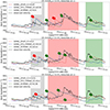 |
Figure 6 Plots of modeled (PFSS + WSA + HUX) and hourly averaged observed solar wind velocity from OMNI database at L1 (solid black line) with time for CR2143 for different Rss, i.e., for Rss = 2.0 R⊙ (top panel), for Rss = 2.5 R⊙ (middle panel) and Rss = 3.0 R⊙ (bottom panel). The red, blue, and green dashed lines show the velocity profiles using HU ZPC, STD, and full ZPC maps, respectively. Green arrows show the time period around which Rss optimization improves the match between the modeled and observed profile as Rss decreases. The red arrows show the time period around which the prediction does not improve as Rss decreases. The shaded regions show the time period where varying Rss significantly changes the modeled velocity profile. |
The green and red shaded areas show the region where using lower Rss improved the solar wind velocity prediction. Green arrows in Figure 6 show the approximate position of the features which matched better with the measurements using lower Rss as compared to higher Rss. As we decrease the Rss from 3.0 R⊙ to 2.0 R⊙ (from bottom panel to top panel), the modeled velocity profile (colored dashed curves) matches better around the green arrows with the measured velocity profile in the red and green shaded areas for all the different maps. The red arrows show the features that matched better with the observation while using higher Rss as compared to lower Rss. However, the overall performance, as indicated in terms of cc, increases as Rss is decreased. For example, for ZPC maps, cc increases from 0.38 to 0.53 and then to 0.6, as Rss decreases from 3.0 R⊙ to 2.5 R⊙ and then to 2.0 R⊙, respectively, as shown in Figure 6. Similar trends can be observed for other maps as well.
It is important to note that although CR2143 shows that the performance improves with decreasing Rss, this does not hold good for all the CRs during the SC24 maximum. However, by examining the average performance based on all the CRs, we can see that lower Rss values (2.0 R⊙ and 2.5 R⊙) perform better than 3.0 R⊙ during SC24 maximum (Fig. 5).
3.2.2 CR2183 (SC24 declining phase)
Rss optimization during the CR2183 gave us better and clearer results about the effects of Rss on the modeled solar wind profile at L1 than CR2143. This is because the PFSS extrapolation during this phase is more reliable than the maximum phase of the SC. Figure 7 shows the modeled (dashed red, green, and blue curves) and observed solar wind velocity profiles (solid black curve) during CR2183.
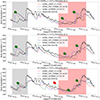 |
Figure 7 Plots of modeled (PFSS+WSA+HUX) and hourly averaged observed solar wind velocity from OMNI database at L1 with time for CR2183 for different Rss, i.e., for Rss = 2.0 R⊙ (top panel), for Rss = 2.5 R⊙ (middle panel), and Rss = 3.0 R⊙(bottom panel). The red, blue, and green dashed lines show the velocity profile using HU ZPC, STD, and full ZPC maps, respectively. Green arrows show the time period around which Rss optimization improves the match between the modeled and observed profile as Rss increases. The red arrows show the time period around which the prediction does not improve as Rss increases. The shaded regions show the time period where Rss significantly changes the modeled velocity profile. |
One can see that increasing the values of the Rss (from top to bottom panels) suppresses most of the additional peaks, as shown by the green arrows, in the modeled solar wind velocity profile, resulting in a better match of the modeled solar wind velocity profile (red, blue and green curves) with the observed profile (black curve). For example, for ZPC maps, cc increases from 0.53 to 0.73 and then to 0.78, as Rss increases from 2.0 R⊙ to 2.5 R⊙ and then to 3.0 R⊙, respectively, as shown in Figure 7. Similar trends can be observed for other maps as well.
The white region between grey and red shaded areas shows a very minute improvement at lower Rss. This is very small in comparison to the improvement at higher Rss in the red and grey-shaded regions. Therefore, the framework performed better at higher Rss, i.e., Rss = 3.0 R⊙.
3.3 Comparing PFSS extrapolation with PROBA2/SWAP observations
In Section 3.1, we observed that using ZPC maps improved the overall performance (averaged over all the three Rss and all CRs) of the framework. This improvement with ZPC maps, compared to STD maps, is evident from the increase in the average cc, computed for all three values of Rss. During the minimum phase of SC24, the average cc increases from 0.31 (for STD maps) to 0.51 (for ZPC maps), and during the maximum phase of SC24, it rises from 0.22 to 0.47, using the default WSA parameters. Similar results for optimized WSA parameters were found, as discussed above, i.e., an increase in average cc from 0.57 to 0.69 during SC24 maximum and an increase in average cc from 0.53 to 0.66 during SC24 minimum (for full CR maps).
This indicates that PFSS extrapolations from ZPC maps are likely to provide a more accurate representation of the magnetic field structure of the Sun compared to the extrapolation from STD GONG maps.
Therefore, we compare the overall large-scale coronal structure during the minimum and maximum phases of the SC with the PFSS extrapolated structure from HU STD and ZPC maps. For this purpose, we used the SWAP mosaics reconstructed from the special observational campaign (discussed in Sect. 2) on 20 August 2017 (CR2194, SC24 minimum) and 7 August 2023 (CR2274, SC25 maximum).
Figure 8 illustrates the observed global coronal structure of the Sun from the PROBA2/SWAP during the minimum of the SC24 on August 20, 2017, 10:45 UT (average time of mosaic). We overlaid magnetic field lines obtained from the PFSS extrapolation using the HU STD map (August 20, 2017, 12:14 UT, top panel) and HU ZPC map (August 20, 2017, 12:14 UT, bottom panel). While the overall structure of the extrapolated field lines obtained from both extrapolations is similar, notable differences can be seen near the south pole (in the zoomed-in panel). In this region, the PFSS extrapolation using the HU ZPC map indicates open field lines (red color field lines), whereas the HU STD map show closed fields (green lines). Upon closer inspection in this region, we can identify a coronal hole in the SWAP images, which agrees with the PFSS extrapolation in the HU ZPC map, indicating open field lines (red color).
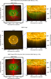 |
Figure 8 PFSS extrapolated magnetic field lines overlaid on the SWAP (top and bottom panel) image of 20 August 2017, 10:45 UT. The middle panel shows the SWAP mosaic without PFSS extrapolation. The top left panel shows PFSS extrapolation with HU STD map, and the bottom left panel with HU ZPC map (on 20 August 2017, 12:14 UT). The right column shows the zoomed-in version of the white rectangle on the left panels. |
Similarly, we compared the extended FOV of SWAP with PFSS extrapolation near the maximum of the SC25 on 7 August 2023 (20:37 UT) (Fig. 9, zoomed-in panels). We can see multiple coronal loop structures all over the western limb in the middle panel of Figure 9. The features in the northwest and southwest limb match better with the PFSS extrapolation with the HU ZPC map in the bottom panel of Figure 9 compared to the HU STD GONG map (top panel of Fig. 9). PFSS extrapolation with HU ZPC map (bottom panel) shows multiple local coronal loops, which are closer to the observations in the middle panel compared to more global coronal loops with HU STD map (top panel). Moreover, near the south pole (zoomed-in panel), the PFSS extrapolation from HU ZPC map exhibits more closed field lines (bottom panel) compared to the HU STD map (top panel). Upon closer examination of the SWAP mosaic (middle panel), a coronal cavity is observed at the south-west limb of the Sun. This rules out the presence of open field lines in this region. The closed field lines are not very prominent in the extrapolation from the HU STD map, where the field lines connect to a larger coronal loop structure/streamer (top panel). The overlying closed loops are distinctly visible in the extrapolation from the HU ZPC map (bottom panel).
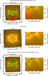 |
Figure 9 PFSS extrapolated magnetic field lines overlaid on PROBA2/SWAP images recorded on 7 August 2023, 20:37 UT. The top panel shows PFSS extrapolation with HU STD maps, and the bottom panel with HU ZPC maps. The middle panel shows the SWAP mosaic without PFSS extrapolation. The right panel shows the zoomed-in version of the white rectangle on the left panel. |
Consequently, from the comparison with SWAP observations, we found that HU ZPC map are a better choice for both the SC minimum, i.e., August 2017, and as well as for the SC maximum, i.e., August 2023, implying that HU ZPC map yield more accurate results in PFSS extrapolation, matching the coronal structure observed in 174 Å. This further resulted in accurate solar wind velocity prediction at L1. Studies by Nikolić (2019) and Li et al.(2021) demonstrated that standard GONG maps used in space weather prediction have shown a decline in accuracy over time because of the PFSS solutions derived from GONG maps, particularly in the polar regions. As mentioned in Section 2, HU ZPC GONG maps mitigate the zero-point inaccuracies. Our analysis of the 16 CRs at different phases of the SC shows that these inaccuracies are crucial in estimating the solar wind velocity of the WSA model at L1. Therefore, we suggest ZPC maps should be used as input in space weather prediction models.
4 Conclusions
In the present study, we estimated the optimal value of Rss for modeling solar wind velocity by using three different types of magnetic maps as inputs for 16 CRs selected at different phases of the SC. We employed two approaches, one using default WSA parameters and the other using a range of WSA parameters to find the best values of Rss among 2.0 R⊙, 2.5 R⊙, and 3.0 R⊙. During the declining phase of the SC24, the model framework performed overall (average cc) better compared to the maximum phases of the SC24 and SC25.
Given the complexity of the solar wind velocity prediction problem at L1, we have attempted to assess the change in the source surface height (Rss) and the impact of the usage of different types of GONG maps and WSA model parameters for different phases of the SC. Our results suggest using a higher surface height (3.0 R⊙) in the WSA model during SC minimum as compared to the conventional Rss (2.5 R⊙). In contrast, during maximum phase of SC24, either Rss = 2.0 R⊙ or Rss = 2.5 R⊙ are found to be preferable. During the SC25 maximum, our results are inconclusive because of the poor performance of the framework.
The results agree with those obtained in previous studies (Lee et al., 2011; Arden et al., 2014), in terms of the relative changes in the best source surface heights with the phase of the SC. Previous studies were based on open magnetic flux estimation at L1. We also want to emphasize that our finding for the SC maximum should be carefully interpreted, keeping in mind the applicability of PFSS during the SC maximum as discussed by Lee et al. (2011).
Our previous study (Kumar & Srivastava, 2022) showed that adding the Schatten Current Sheet (SCS; Schatten, 1971) model to the approach provides a similar performance of the framework. Current work hints towards the need for optimization of source surface height in the PFSS model in the context of its use in the WSA model. At the same time, the study highlights the difficulties due to the limitations of the PFSS model during the solar maximum and uncertainties in the magnetic field measurements at the poles.
We want to mention here that standard magnetic maps from GONG have been used extensively by the community in solar wind velocity forecasting frameworks, e.g., Shiota et al. (2014); Pomoell & Poedts (2018); Nikolić (2019); Narechania et al. (2021); Kumar & Srivastava (2022); Mayank et al. (2022). They are also used in operational WSA-ENLIL simulations. However, we found substantial improvement in the performance of the solar wind forecasting framework while using ZPC magnetic maps compared to STD maps, which is further confirmed by the comparison of PFSS extrapolation with the near-Sun observations obtained from the SWAP instrument. It thus establishes a link between the quality of near-Sun PFSS extrapolation and the quality of solar wind velocity prediction at L1. Therefore, we strongly advocate the use of ZPC magnetic maps from GONG in space weather prediction models instead of standard maps. A previous study by Narechania et al. (2021) supported the use of ZPC maps compared to the STD GONG maps based on a single case study using MHD simulations.
Our study further supports their results based on a more robust and long-term analysis at different phases of the SC. Moreover, we validated the superiority of ZPC maps over standard GONG maps in both PFSS extrapolations compared with near-Sun observations, and as input in solar wind velocity prediction models at L1. A recent study by Li et al. (2021) based upon open flux and polarity of the IMF at L1 reported that ZPC maps outperformed standard GONG maps significantly. However, they also found that HMI maps (cc = 0.71) performed slightly better than ZPC maps (cc = 0.70) when compared with observed open flux. A more recent study by Mayank et al. (2022) reported that in the context of solar wind prediction at L1, GONG standard maps outperformed the HMI maps for CR2104 (ascending phase of the SC24). They did not use ZPC GONG maps in their study. Therefore, further investigation is required to compare the impact of different magnetic maps in the context of solar wind velocity prediction.
Our study used discrete sets of 4 CRs (in total 16 CRs) at different SC phases and three distinct values of Rss. Our work is the first step and points out the potential ways to improve the framework. Therefore, to further verify the applicability of the results over the entire phases of the SC, a long-term continuous study is required with a more refined choice of Rss.
It is also important to mention that we used the HUX model for solar wind velocity extrapolation for simplicity. However, a slightly advanced version of this model, i.e., HUXt (Barnard & Owens, 2022), could be used in future work to provide a more realistic framework. This model introduces an explicit time dependence in the solar wind extrapolation by introducing a residual acceleration in the solar wind. Further, the optimization approach relying solely on Pearson’s coefficient has its own drawbacks as it disregards other metrics and does not account for overall features. Therefore, advanced metrics, e.g., Dynamic Time warping (Samara et al., 2022) or a combination of metrics, can be used to obtain more robust and conclusive results.
Badman et al. (2020) suggested the use of lower surface height (1.3–1.5 R⊙) to reproduce the radial component of the magnetic field observed at PSP located at 0.5 AU on specific days (2018-10-20 and 2018-10-29), which depends upon the connectivity of the magnetic field lines and the local magnetic field distribution. Our approach in the current work is to optimize the source surface height, i.e., Rss for the entire CR and compare observed and modeled solar wind velocity at L1 for each CR. It may be noted that in our study during solar minimum, for some specific short time periods (during individual CRs), we found that the modeled solar wind velocity profile for lower Rss values matches better with the observed profile (Sect. 3.2). Nevertheless, a higher Rss (3.0 R⊙) was found to perform better for the entire CR as inferred from the cc value. And the opposite was observed during SC maximum.
The study by Huang et al. (2024) suggested a slightly lower Rss than 2.5 R⊙ during a solar minimum, by comparing the unsigned, open flux at L1. It assumes an isotropic magnetic field in the heliosphere. This approach is sensitive to the area of coronal holes only, whereas our study is complex in the sense that our final modeled output, the velocity at L1, is related to the overall area of the coronal holes, the overall structure, and connectivity of sub-Earth field lines on the solar surface. Moreover, we use a more sophisticated extrapolation (HUX) method in the heliosphere than previous studies. Therefore, our study highlights the challenges and intricacy of the problem in optimising the source surface height in the PFSS model while using different approaches.
Based on the encouraging results of the current study, which was limited by the availability of the SWAP mosaic data collected during two phases (CR2194, Aug 2017 and CR2274, Aug 2023) of the recent SC, the PROBA2 team has scheduled special observational campaigns every month since. These will be used to test and validate future data sets for more quantitative comparisons.
In summary, the present work is a first step in the direction of improving the WSA model and points out the potential ways to enhance the PFSS+WSA framework of solar wind forecasting at L1. For this purpose, we explore the use of different values of the source surface height (Rss) and different kinds of maps in the PFSS model during selected time periods. This knowledge can contribute to refining predictions of solar wind velocity, as well as for operational space weather frameworks.
Acknowledgments
We thank the reviewers and the editor for the constructive comments to improve the manuscript. The authors have used pfsspy (Stansby et al., 2020). The data used in this study are all publicly available. We want to acknowledge the GONG group for magnetic synoptic maps available on https://gong2.nso.edu/archive/patch.pl?menutype=zeroPoint#step2. Solar wind velocity data is available on https://omniweb.gsfc.nasa.gov/form/dx1.html. The sunspot data is courtesy of WDC-SILSO, Royal Observatory of Belgium, Brussels. We acknowledge the Sunpy community (The SunPy Community et al., 2020). SK and NS want to express their gratitude for the support received through the PROBA2 Guest Investigator program grant. S.K and N.S. also want to express special thanks to the PROBA2 operational team for conducting a special campaign of SWAP observations to have an extended FOV. SWAP is a project of the Centre Spatial de Liége and the Royal Observatory of Belgium, funded by the Belgian Federal Science Policy Office (BELSPO). The ROB team thanks the Belgian Federal Science Policy Office (BELSPO) for the provision of financial support in the framework of the PRODEX Programme of the European Space Agency (ESA). The editor thanks Eleanna Asvestari and an anonymous reviewer for their assistance in evaluating this paper.
Appendix
Figures 10 and 11 illustrate the MAPE for different CRs with different Rss in the first and second approaches, respectively. It is evident that the average MAPE has increased significantly for the SC25 maximum (rightmost column of both Figures) in the second approach compared to the first.
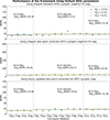 |
Figure A1 Mean Absolute Percentage Error (MAPE) for different CRs with different Rss based on default WSA parameters. The top panel shows the result using standard Carrington maps (STD), the middle panel is for the zero-point corrected Carrington maps (ZPC), and the bottom panel is for zero-point corrected hourly updated maps (HU ZPC). Blue, orange, and green dots represent the performance of the framework for Rss of 2.0 R⊙, 2.5 R⊙, and 3.0 R⊙, respectively. Horizontal dashed lines show the average performance in the respective phase for each Rss and all CRs. An annotated average MAPE for each phase shows the aggregate average values for all the three Rss. |
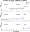 |
Figure A2 Similar to Figure A1. Corresponding to optimized WSA parameters, i.e., WSA parameters corresponding to highest cc. It may be noted that MAPE values for CR2275 using the ZPC map (middle panel) are in the range of 300–400 and, therefore, can not be shown in the selected limit of the y-axis. |
In contrast, the MAPE values for the SC24 maximum and declining phase did not increase as significantly. Specifically, for ZPC maps in the SC24 declining phase, MAPE increased moderately from 20% to 25%. However, for the SC25 maximum, the increase was much more pronounced, rising from 22% to 114% (average for all three Rss values) in Figure 11 compared to Figure 10.
References
- Alissandrakis CE. 1981. On the computation of constant alpha force-free magnetic field. A&A 100(1): 197–200. [Google Scholar]
- Arden WM, Norton AA, Sun X. 2014. A “breathing” source surface for cycles 23 and 24. J Geophys Res Space Phys 119(3): 1476–1485. https://doi.org/10.1002/2013JA019464. [CrossRef] [Google Scholar]
- Arge CN, Odstrcil D, Pizzo VJ, Mayer LR. 2003. Improved method for specifying solar wind speed near the sun. In: Solar wind ten, vol. 679 of American Institute of Physics Conference Series, Velli M, Bruno R, Malara F, Bucci B (Eds.), AIP: Pisa, pp. 190–193. https://doi.org/10.1063/1.1618574. [Google Scholar]
- Arge CN, Pizzo CN. 2000. Improvement in the prediction of solar wind conditions using near-real time solar magnetic field updates, J Geophys Res , 105(A5): 10465–10480. https://doi.org/10.1029/1999JA000262. [CrossRef] [Google Scholar]
- Badman ST, Bale SD, Martínez Oliveros JC, Panasenco O, Velli M, et al. 2020. Magnetic connectivity of the ecliptic plane within 0.5 au: potential field source surface modeling of the first parker solar probe encounter. Astrophys J Suppl Ser 246(2): 23. https://doi.org/10.3847/1538-4365/ab4da7. [CrossRef] [Google Scholar]
- Barnard L, Owens M. 2022. HUXt – an open source, computationally efficient reduced-physics solar wind model, written in Python. Front Phys 10, 1005621. https://doi.org/10.3389/fphy.2022.1005621. [CrossRef] [Google Scholar]
- Berghmans D, Hochedez J, Defise J, Lecat J, Nicula B, et al. 2006. SWAP onboard PROBA 2, a new EUV imager for solar monitoring. Adv Space Res 38(8): 1807–1811. Magnetospheric dynamics and the international living with a star program. https://doi.org/10.1016/j.asr.2005.03.070. [CrossRef] [Google Scholar]
- Fox NJ, Velli MC, Bale SD, Decker R, Driesman A, et al. 2016. The solar probe plus mission: humanity’s first visit to our star. Space Sci Rev 204(1–4): 7–48. https://doi.org/10.1007/s11214-015-0211-6. [CrossRef] [Google Scholar]
- Halain JP, Berghmans D, Seaton DB, Nicula B, De Groof A, Mierla M, Mazzoli M, Defise JM, Rochus P. 2013. The SWAP EUV imaging telescope. Part II: in-flight performance and calibration. Solar Phys 286(1): 67–91. https://doi.org/10.1007/s11207-012-0183-6. [CrossRef] [Google Scholar]
- He H, Wang H, Yan Y. 2011. Nonlinear force-free field extrapolation of the coronal magnetic field using the data obtained by the Hinode satellite. J Geophys Res Space Phys 116(A1):, A01101. https://doi.org/10.1029/2010JA015610. [Google Scholar]
- Hill F. 2018. The global oscillation network group facility – an example of research to operations in space weather, Space Weather 16(10): 1488–1497. https://doi.org/10.1029/2018SW002001. [NASA ADS] [CrossRef] [Google Scholar]
- Huang Z, Tóth G, Huang J, Sachdeva N, van der Holst B, Manchester WB. 2024. Adjusting the potential field source surface height based on magnetohydrodynamic simulations. Astrophys J Lett 965(1): L1. https://doi.org/10.3847/2041-8213/ad3547. [CrossRef] [Google Scholar]
- Kruse M, Heidrich-Meisner V, Wimmer-Schweingruber RF, Hauptmann M. 2020. An elliptic expansion of the potential field source surface model. A&A 638: A109. https://doi.org/10.1051/0004-6361/202037734. [NASA ADS] [CrossRef] [EDP Sciences] [Google Scholar]
- Kumar S, Paul A, Vaidya B. 2020. A comparison study of extrapolation models and empirical relations in forecasting solar wind. Front Astron Space Sci , 7: 92. https://doi.org/10.3389/fspas.2020.572084. [CrossRef] [Google Scholar]
- Kumar S, Srivastava N. 2022. A parametric study of performance of two solar wind velocity forecasting models during 2006–2011. Space Weather 20(9): e2022SW003069. https://doi.org/10.1029/2022SW003069. [CrossRef] [Google Scholar]
- Lee CO, Luhmann JG, Hoeksema JT, Sun X, Arge CN, de Pater I. 2011. Coronal field opens at lower height during the solar cycles 22 and 23 minimum periods: imf comparison suggests the source surface should be lowered. Solar Phys 269(2): 367–388. https://doi.org/10.1007/s11207-010-9699-9. [CrossRef] [Google Scholar]
- Li H, Feng X, Wei F. 2021. Comparison of synoptic maps and PFSS solutions for the declining phase of solar cycle 24. J Geophys Res Space Phys 126(3): e28870. https://doi.org/10.1029/2020JA028870. [Google Scholar]
- Lowder C, Qiu J, Leamon R. 2017. Coronal holes and open magnetic flux over cycles 23 and 24. Solar Phys 292(1): 18. https://doi.org/10.1007/s11207-016-1041-8. [CrossRef] [Google Scholar]
- Mayank P, Vaidya P, Chakrabarty D. 2022. SWASTi-SW: space weather adaptive simulation framework for solar wind and its relevance to the Aditya-L1 mission. Astrophys J Suppl Ser , 262(1): 23. https://doi.org/10.3847/1538-4365/ac8551. [CrossRef] [Google Scholar]
- Meyer KA, Mackay DH, TalpeanuD-C, Upton LA, West MJ. 2020. Investigation of the middle corona with SWAP and a data-driven non-potential coronal magnetic field model. Solar Phys 295(7): 101. https://doi.org/10.1007/s11207-020-01668-2. [CrossRef] [Google Scholar]
- Narechania NM, Nikolić L, Freret L, De Sterck H, Groth CPT. 2021. An integrated data-driven solar wind – CME numerical framework for space weather forecasting. J Space Weather and Space Clim 11: 8. https://doi.org/10.1051/swsc/2020068. [CrossRef] [EDP Sciences] [Google Scholar]
- Nikolić L. 2019. On solutions of the PFSS model with GONG synoptic maps for 2006–2018. Space Weather 17(8): 1293–1311. https://doi.org/10.1029/2019SW002205. [CrossRef] [Google Scholar]
- Odstrcil D, Riley P, Zhao XP. 2004. Numerical simulation of the 12 May 1997 interplanetary CME event. J Geophys Res Space Phys 109(A2): A02116. https://doi.org/10.1029/2003JA010135. [CrossRef] [Google Scholar]
- Perri B, Leitner P, Brchnelova M, Baratashvili T, Kuzma B, Zhang F, Lani A, Poedts S. 2022. COCONUT, a novel fast-converging MHD model for solar corona simulations: I. Benchmarking and optimization of polytropic solutions. Astrophys J 936(1): 19. https://doi.org/10.3847/1538-4357/ac7237. [CrossRef] [Google Scholar]
- Pomoell J, Poedts S. 2018. EUHFORIA: European heliospheric forecasting information asset. J Space Weather Space Clim 8: A35. https://doi.org/10.1051/swsc/2018020. [Google Scholar]
- Reiss MA, MacNeice PJ, Mays LM, Arge CN, Möstl C, Nikolić L, Amerstorfer T. 2019. Forecasting the ambient solar wind with numerical models. I. On the implementation of an operational framework. Astrophys J Suppl Ser 240(2): 35. https://doi.org/10.3847/1538-4365/aaf8b3. [CrossRef] [Google Scholar]
- Riley P, Linker JA, Arge CN. 2015. On the role played by magnetic expansion factor in the prediction of solar wind speed. Space Weather 13(3): 154–169. https://doi.org/10.1002/2014SW001144. [NASA ADS] [CrossRef] [Google Scholar]
- Riley P, Linker JA, Mikić Z. 2001. An empirically-driven global MHD model of the solar corona and inner heliosphere. J Geophys Res Space Phys 106(8): 15889–15901. https://doi.org/10.1029/2000JA000121. [CrossRef] [Google Scholar]
- Riley P, Lionello R. 2011. Mapping solar wind streams from the sun to 1 au: a comparison of techniques. Solar Phys 270(2): 575–592. https://doi.org/10.1007/s11207-011-9766-x. [CrossRef] [Google Scholar]
- Samara E, Laperre B, Kieokaew R, Temmer M, Verbeke C, Rodriguez L, Magdalenic J, Poedts S. 2022. Dynamic time warping as a means of assessing solar wind time series. Astrophys J 927(2): 187. https://doi.org/10.3847/1538-4357/ac4af6. [CrossRef] [Google Scholar]
- Santandrea S, Gantois K, Strauch K, Teston F, Proba2 Project Team, et al. 2013. PROBA2: Mission and spacecraft overview Solar Phys 286(1): 5–19. https://doi.org/10.1007/s11207-013-0289-5. [CrossRef] [Google Scholar]
- Schatten KH. 1971. Current sheet magnetic model for the solar corona. Cosmic Electrodyn 2: 232–245. [Google Scholar]
- Schatten KH, Wilcox JM, Ness NF. 1969. A model of interplanetary and coronal magnetic fields. Solar Phys 6(3): 442–455. https://doi.org/10.1007/BF00146478. [CrossRef] [Google Scholar]
- Scherrer PH, Bogart RS, Bush RI, Hoeksema JT, Kosovichev AG, et al. 1995. The solar oscillations investigation – Michelson Doppler Imager. Solar Phys 162(1–2): 129–188. https://doi.org/10.1007/BF00733429. [CrossRef] [Google Scholar]
- Scherrer PH, Schou J, Bush RI, Kosovichev AG, Bogart RS, et al. 2012. The Helioseismic and Magnetic Imager (HMI) investigation for the solar dynamics observatory (SDO). Solar Phys 275(1–2): 207–227. https://doi.org/10.1007/s11207-011-9834-2. [CrossRef] [Google Scholar]
- Seaton DB, Berghmans D, Nicula B, Halain JP, De Groof A, et al. 2013. The SWAP EUV imaging telescope part I: instrument overview and pre-flight testing. Solar Phys 286(1): 43–65. https://doi.org/10.1007/s11207-012-0114-6. [CrossRef] [Google Scholar]
- Shiota D, Kataoka R, Miyoshi Y, Hara Y, Tao C, Masunaga K, Futaana Y, Terada N. 2014.Inner heliosphere MHD modeling system applicable to space weather forecasting for the other planets. Space Weather 12(4): 187–204. https://doi.org/10.1002/2013SW000989. [NASA ADS] [CrossRef] [Google Scholar]
- Stansby D, Yeates A, Badman ST. 2020. pfsspy: a Python package for potential field source surface modelling. J Open Source Soft 5(54): 2732. https://doi.org/10.21105/joss.02732. [CrossRef] [Google Scholar]
- The SunPy Community, Barnes WT, Bobra MG, Christe SD, Freij N, et al. 2020. The SunPy Project: open source development and status of the version 1.0 core package. Astrophys J 890: 68. https://doi.org/10.3847/1538-4357/ab4f7a. [CrossRef] [Google Scholar]
- van der Holst B, Sokolov IV, Meng X, Jin M, Manchester IV WB, Tóth G, Gombosi TI. 2014. Alfvén Wave Solar Model (AWSoM): coronal heating. Astrophys J 782(2): 81. https://doi.org/10.1088/0004-637X/782/2/81. [CrossRef] [Google Scholar]
- Wang YM, Sheeley Jr NR. 1990. Solar wind speed and coronal flux-tube expansion. Astrophys J 355: 726. https://doi.org/10.1086/168805. [CrossRef] [Google Scholar]
- West MJ, Seaton DB, D’Huys E, Mierla M, Laurenza M, Meyer KA, Berghmans D, Rachmeler LR, Rodriguez L, Stegen K. 2022. A review of the extended EUV corona observed by the sun watcher with active pixels and image processing (SWAP) instrument. Solar Phys 297(10): 136. https://doi.org/10.1007/s11207-022-02063-9. [CrossRef] [Google Scholar]
- Wiegelmann T. 2004. Optimization code with weighting function for the reconstruction of coronal magnetic fields. Solar Phys 219(1): 87–108. https://doi.org/10.1023/B:SOLA.0000021799.39465.36. [CrossRef] [Google Scholar]
Cite this article as: Kumar S, Srivastava N, Talpeanu D, Mierla M, D’Huys E, et al. 2025. On the role of source surface height and magnetograms in solar wind forecast accuracy. J. Space Weather Space Clim. 15, 24. https://doi.org/10.1051/swsc/2025021.
All Tables
All Figures
|
Figure 1 Monthly sunspot numbers (blue line) plotted with time, indicating different phases of solar activity cycle 24 and 25. Vertical lines mark the CRs selected for analysis at different phases of the SC. |
| In the text | |
|
Figure 2 Flow chart of the methodology adopted in this work to find optimal Rss. Steps mentioned in the magenta colour box are repeated for all three choices of Rss, i.e., 2.0 R⊙, 2.5 R⊙, and 3.0 R⊙. |
| In the text | |
|
Figure 3 The performance of the framework (cc) for different CRs with different Rss based on default WSA parameters. For SC24, refer to the left y-axis, whereas for SC25 maximum, refer to the right y-axis in red. The top panel shows the result using standard Carrington maps (STD), the middle panel is for the zero-point corrected Carrington maps (ZPC), and the bottom panel is for hourly updated zero-point corrected maps (HU ZPC). Blue, orange, and green dots represent the performance of the framework, i.e., cc, for Rss of 2.0 R⊙, 2.5 R⊙, and 3.0 R⊙, respectively. Horizontal dashed lines show the average performance in the respective phase for each Rss and all CRs. The annotated value shows the average value of cc for each input map and SC phase for all three Rss (dashed lines). |
| In the text | |
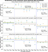 |
Figure 4 Similar to Figure 3 for optimised WSA parameters. |
| In the text | |
|
Figure 5 Number of cases for different Rss in the best-performing scenario during the selected phase of the SC. Note, as explained in Section 3, the framework performed poorly for the SC25 maximum phase. Therefore, the results from the right panel are inconclusive. |
| In the text | |
|
Figure 6 Plots of modeled (PFSS + WSA + HUX) and hourly averaged observed solar wind velocity from OMNI database at L1 (solid black line) with time for CR2143 for different Rss, i.e., for Rss = 2.0 R⊙ (top panel), for Rss = 2.5 R⊙ (middle panel) and Rss = 3.0 R⊙ (bottom panel). The red, blue, and green dashed lines show the velocity profiles using HU ZPC, STD, and full ZPC maps, respectively. Green arrows show the time period around which Rss optimization improves the match between the modeled and observed profile as Rss decreases. The red arrows show the time period around which the prediction does not improve as Rss decreases. The shaded regions show the time period where varying Rss significantly changes the modeled velocity profile. |
| In the text | |
|
Figure 7 Plots of modeled (PFSS+WSA+HUX) and hourly averaged observed solar wind velocity from OMNI database at L1 with time for CR2183 for different Rss, i.e., for Rss = 2.0 R⊙ (top panel), for Rss = 2.5 R⊙ (middle panel), and Rss = 3.0 R⊙(bottom panel). The red, blue, and green dashed lines show the velocity profile using HU ZPC, STD, and full ZPC maps, respectively. Green arrows show the time period around which Rss optimization improves the match between the modeled and observed profile as Rss increases. The red arrows show the time period around which the prediction does not improve as Rss increases. The shaded regions show the time period where Rss significantly changes the modeled velocity profile. |
| In the text | |
|
Figure 8 PFSS extrapolated magnetic field lines overlaid on the SWAP (top and bottom panel) image of 20 August 2017, 10:45 UT. The middle panel shows the SWAP mosaic without PFSS extrapolation. The top left panel shows PFSS extrapolation with HU STD map, and the bottom left panel with HU ZPC map (on 20 August 2017, 12:14 UT). The right column shows the zoomed-in version of the white rectangle on the left panels. |
| In the text | |
|
Figure 9 PFSS extrapolated magnetic field lines overlaid on PROBA2/SWAP images recorded on 7 August 2023, 20:37 UT. The top panel shows PFSS extrapolation with HU STD maps, and the bottom panel with HU ZPC maps. The middle panel shows the SWAP mosaic without PFSS extrapolation. The right panel shows the zoomed-in version of the white rectangle on the left panel. |
| In the text | |
|
Figure A1 Mean Absolute Percentage Error (MAPE) for different CRs with different Rss based on default WSA parameters. The top panel shows the result using standard Carrington maps (STD), the middle panel is for the zero-point corrected Carrington maps (ZPC), and the bottom panel is for zero-point corrected hourly updated maps (HU ZPC). Blue, orange, and green dots represent the performance of the framework for Rss of 2.0 R⊙, 2.5 R⊙, and 3.0 R⊙, respectively. Horizontal dashed lines show the average performance in the respective phase for each Rss and all CRs. An annotated average MAPE for each phase shows the aggregate average values for all the three Rss. |
| In the text | |
|
Figure A2 Similar to Figure A1. Corresponding to optimized WSA parameters, i.e., WSA parameters corresponding to highest cc. It may be noted that MAPE values for CR2275 using the ZPC map (middle panel) are in the range of 300–400 and, therefore, can not be shown in the selected limit of the y-axis. |
| In the text | |
Current usage metrics show cumulative count of Article Views (full-text article views including HTML views, PDF and ePub downloads, according to the available data) and Abstracts Views on Vision4Press platform.
Data correspond to usage on the plateform after 2015. The current usage metrics is available 48-96 hours after online publication and is updated daily on week days.
Initial download of the metrics may take a while.