| Issue |
J. Space Weather Space Clim.
Volume 15, 2025
Topical Issue - Observing, modelling and forecasting TIDs and mitigating their impact on technology
|
|
|---|---|---|
| Article Number | 25 | |
| Number of page(s) | 19 | |
| DOI | https://doi.org/10.1051/swsc/2025020 | |
| Published online | 03 July 2025 | |
Technical Article
An explainable Machine Learning model for Large-Scale Travelling Ionospheric Disturbances forecasting
1
Istituto Nazionale di Geofisica e Vulcanologia, Via di Vigna Murata 605, 00143 Rome, Italy
2
Sapienza Università di Roma, Piazzale Aldo Moro 5, 00185 Rome, Italy
3
Observatori de l’Ebre, University Ramon Llull – CSIC, Ctra. de l'Observatori 3, 43520 Roquetes, Tarragona, Spain
4
University of Massachusetts Lowell, 220 Pawtucket St, Lowell, 01854 MA, USA
5
HUN-REN Institute of Earth Physics and Space Science, Csatkai E. u. 6-8., 9400 Sopron, Hungary
6
Royal Meteorological Institute of Belgium, Solar Terrestrial Centre of Excellence, Av. Circulaire 3, BE-1180 Brussels, Belgium
7
National Observatory of Athens, IAASARS, Vas. Pavlou & I. Metaxa, GR-15 236 Penteli, Greece
* Corresponding author: This email address is being protected from spambots. You need JavaScript enabled to view it.
; This email address is being protected from spambots. You need JavaScript enabled to view it.
Received:
27
August
2024
Accepted:
7
May
2025
Abstract
Large-Scale Travelling Ionospheric Disturbances (LSTIDs) are wave-like ionospheric fluctuations, generally triggered by geomagnetic storms, which play a critical role in space weather dynamics. In this work, we present a machine learning model able to forecast the occurrence of LSTIDs over the European continent up to three hours in advance. The model is based on CatBoost, a gradient boosting framework. It is trained on a human-validated LSTID catalogue with the various physical drivers, including ionogram information, geomagnetic, and solar activity indices. There are three forecasting modes depending on the demanded scenarios with varying relative costs of false positives and false negatives. It is crucial to make the model predictions explainable, so that the output contribution of each physical factor input is visualised through the game-theoretic SHapley Additive exPlanation (SHAP) formalism. The validation procedure consists of a global-level evaluation and interpretation step, firstly, followed by an event-level validation against independent detection methods, which highlights the model’s predictive robustness and suggests its potential for real-time space weather forecasting. Depending on the operating mode, we report an improvement ranging from +72% to +93% over the performance of a rule-based benchmark. Our study concludes with a comprehensive analysis of future research directions and actions to be taken towards full operability. We discuss probabilistic forecasting approaches from a cost-sensitive learning perspective, along with performance-centric model monitoring. Finally, through the lens of the conformal prediction framework, we further comment on the uncertainty quantification for end-user risk management and mitigation.
Key words: Large Scale Travelling Ionospheric Disturbances / Ionosphere / Forecasting / Explainable Artificial Intelligence / Machine Learning
© V. Ventriglia et al., Published by EDP Sciences 2025
 This is an Open Access article distributed under the terms of the Creative Commons Attribution License (https://creativecommons.org/licenses/by/4.0), which permits unrestricted use, distribution, and reproduction in any medium, provided the original work is properly cited.
1 Introduction
1.1 Real-time TID monitoring
Travelling Ionospheric Disturbances (TIDs) are one of the phenomena responsible for the degradation of GNSS positioning quality, they have an impact on radio communication and direction-finding radar precision. Thus, in addition to being of scientific interest, they have been studied for many decades to mitigate their impact (Hines, 1960; Chan & Villard, 1962; Davis, 1971; Hunsucker, 1982; Afraimovich et al., 2000). TIDs are usually the ionospheric signature of atmospheric gravity waves (AGWs) propagating in the thermosphere. Anyhow, some TIDs are generated by other phenomena, such as Perkins instability (Makela & Otsuka, 2012). TIDs are generally classified according to their physical characteristics, such as group velocity, period, azimuth, amplitude, and wavelength (Georges, 1968; Hunsucker, 1982). The two most studied kinds of TIDs are medium-scale (MSTIDs) and large-scale (LSTIDs), categorised by their spatial scales. Most MSTIDs have horizontal velocities between 100 and 250 m/s, wavelengths in the order of several hundred kilometres, and a period of 15–60 minutes. On the other hand, LSTIDs are defined by a horizontal scale of more than 1000 km, speeds between 400 and 1000 km and periods in the 30–180 min range. LSTIDs are usually produced in the auroral oval during the enhanced periods of geomagnetic storms, then propagate equatorward along the field lines. Although the exact physical generation mechanism of LSTIDs is still not fully understood, one possible cause may be the AGWs generated by the thermospheric heating during solar storms. The two processes that contribute to the generation of AGWs are Joule and particle heating (Banks, 1977) and Lorentz forces. According to Oyama & Watkins (2012), Lorentz forces correlate to the increased wind velocity, while Joule and particle heatings are responsible for temperature perturbations. As the auroral electrojet is related to both phenomena, indicators of the strength of such electric current should be representative of LSTID generation. Borries et al. (2009) demonstrated that there is a correlation between the Auroral Electrojet Index (AE) (Kamide & Akasofu, 1983) and the LSTID amplitude. Even if most of LSTID events are related to increased geomagnetic activity and energy injection at high latitudes and thus propagating toward equatorial latitudes, there have been observations of both poleward LSTIDs (Habarulema et al., 2015, 2016; Ngwira et al., 2019) and occurrences during quiet times related to secondary gravity waves generated by deep tropospheric convection (Zhou et al., 2012). MSTIDs are normally observed during both geomagnetically disturbed and quiet times, generated mostly by lower atmospheric (meteorological) sources (see, e.g., Azeem et al., 2015). MSTIDs are also triggered by natural and man-made impulsive events in the lower atmosphere (Hunsucker, 1982), such as earthquakes (Haralambous et al., 2023), volcanic eruptions, tsunamis (Savastano et al., 2017), explosions, or rocket launches. Recently, the MSTIDs generated following the explosion of the Hunga Tonga‐Hunga Ha’apai submarine volcano have attracted much attention in the scientific community (Themens et al., 2022; Verhulst et al., 2022). TIDs can be observed by leveraging different sounding instruments: ionosondes (Bowman, 1965; Maeda & Handa, 1980; Verhulst et al., 2022) and TEC derived from Global Navigation Satellite System (GNSS) (Saito et al., 1998; Zakharenkova et al., 2016; Guerra et al., 2024), which are two of the most widely exploited techniques.
A comprehensive nowcasting system for TIDs has been developed in the frame of the “Warning and Mitigation Technologies for Travelling Ionospheric Disturbances” (TechTIDE) project, funded by the European Commission Horizon 2020 Programme. The TechTIDE services monitor MSTIDs and LSTIDs over Europe in near real-time, implementing a variety of complementary methodologies based on the real-time processing of observations acquired by the ground-based network of GNSS receivers, digisonde stations, and continuous Doppler sounding systems with the corresponding drivers from the near-Earth space and the lower atmosphere (Belehaki et al., 2020). Two examples of TechTIDE nowcasting methodology for TID detection based on high-frequency (HF) measurements are HF-TID and HF Interferometry (HF-INT). The HF-TID method (Huang et al., 2016; Reinisch et al., 2018) leverages Digisonde to Digisonde (D2D) measurements. The method assumes the ionosphere as a moving undulated mirror, which allows the extraction of TID parameters through the Doppler frequency- and angular-sounding technique (Paznukhov et al., 2012). The HF-INT method (Altadill et al., 2020) analyses the time series of parameters derived from single ionosonde measurements. Specifically, it searches for periodic features in the maximum usable frequency (MUF(3000)F2), a parameter that accounts for peak electron density and height. If the method successfully detects periodic features, it proceeds with the cross-correlation of measurements gathered by different ionosondes. By searching for the time lag of max correlation, it is possible to derive the propagation velocity of a TID. In terms of GNSS-based techniques, one of the most widely used techniques to detect LSTID is manually highlighting them in latitudinal keograms (Zakharenkova et al., 2016; Nykiel et al., 2024). In contrast to HF-based techniques, the process here is not autonomous but rather requires human interpretation. Keograms are plots that show the detrended TEC (dTEC) measurements as a function of time and latitude (Eather et al., 1976; Tsugawa et al., 2003). dTEC measurements are usually obtained by applying a detrending technique to the time series of the geometry-free linear combination of phase measurements collected by GNSS geodetic receivers (Afraimovich et al., 2013; Guerra et al., 2024). The three introduced techniques will be leveraged to investigate three specific case events in the validation section.
Besides the scientific interest, TIDs have a disruptive effect on HF communications, HF-based navigation, and GNSS positioning systems (Timoté et al., 2020; Poniatowski & Nykiel, 2020). That is why a strong effort was dedicated to developing near-real-time detection techniques for LSTIDs (Belehaki et al., 2020). However, TIDs and their excitation sources do not have a one-to-one correspondence, so the real-time monitoring and prediction of TIDs based on the physical formation mechanisms remains high difficult. For this reason, there is a demand to create an algorithm that is capable of predicting the occurrence of LSTIDs and provide alerts to help mitigate their impact on the scientific and commercial interests.
1.2 From monitoring to forecasting
Statistical analyses and investigations of the source mechanisms of TIDs have been carried out, showing modelling and prediction capabilities based on a deep learning algorithm for monitoring MSTIDs (Liu et al., 2022). Yet, an accurate forecasting method has not been established. Thus, we turn our attention to the development of a machine learning (ML) model that can leverage different input features, representing geomagnetic and ionospheric conditions. Many different ML models have been used for space weather forecasting applications (Camporeale, 2019). To the best of our knowledge, ML forecasting models related to ionospheric applications have only been developed for TEC and scintillation forecasting (e.g., Cesaroni et al., 2020; McGranaghan et al., 2018; Iban & Şentürk, 2022; Asamoah et al., 2024).
Statistical and ML-based time series forecasting is becoming an increasingly relevant technique in the context of space weather. Statistical methods like autoregressive integrated moving average (ARIMA) can analyse the past ionospheric data to identify trends and periodicities, providing insights for future predictions (Filjar, 2021). Long Short-Term Memory (LSTM) networks handle the sequential nature of time series data, learning complex patterns over time to forecast LSTID occurrence and possibly estimating their intensity, capturing long-term dependencies and non-linearities present in the data (Liu et al., 2020). In the vast landscape of time-series analysis, time-series classification – a task involving training a model from a collection of time series – has recently obtained a lot of attention. Many algorithms are designed to perform time series classification, among which we mention: distance-based approaches (such as k-nearest neighbours, support vector machine, and dynamic time warping), shapelet transforms, dictionary approaches (like ROCKET or Bag-of-Patterns), interval-based approaches (such as time-series forest), deep learning, and model ensembles (such as hierarchical vote collective of transformation-based ensembles).
In this work, we employ a gradient boosting algorithm to face a multivariate time-series classification problem. This approach can be highly effective; however, it requires careful consideration of the specific characteristics that are inherent in the time series data. This class of algorithms provides significant advantages, including the ability to handle heterogeneous data and model complex non-linear relationships. Additionally, they are robust against partly relevant features, which are common in time series data. However, boosting models do not inherently account for the time-ordering and non-stationarity of the data, unless specific preprocessing (e.g., moving averages, differencing) is applied. Model validation is another critical issue, about any ML model applied to time series, since traditional k-fold cross-validation becomes inappropriate due to the temporal dependency.
The research described in this paper was conducted in the context of the EU-funded Travelling Ionospheric Disturbances Forecasting System (T-FORS) project. T-FORS aims at providing new models able to interpret a broad range of physical observations, and issue forecasts and warnings for LSTIDs several hours before their onset. Within the project, different prediction approaches are selected for LSTIDs and MSTIDs in recognition of their different origins and mechanisms of generation. Regarding LSTIDs, ML models were trained on existing databases to estimate their probability of occurrence.
The paper is organised as follows: Section 2 describes the data used and their pre-processing, the model characteristics, including its various configurations, and the explainability framework. Section 3 provides a detailed discussion of model training and validation, both globally and on an event-based level. Section 4 discusses the feasibility of integrating the model into an operational framework. Finally, Section 5 presents the conclusions.
2 Data and methods
The main objective of the model presented in this paper is to predict the occurrence of LSTIDs over Europe. The model faces the complexity of the physical processes leading to the generation and propagation of LSTIDs through the solar wind, the magnetosphere, and the high-latitude ionosphere. The challenge is to provide forecasting of LSTIDs occurrences with a proper time horizon, namely up to three hours ahead. A model that only has input on the temporal evolution of physical observables deemed important for the study of the phenomenon, and not spatial data, can only make predictions in an “average” sense. This is why we will treat the problem as if everything were concentrated around a point located at 50° latitude and 9° longitude (which identifies roughly the barycentre of the European continent), even though an LSTID is not such a localised phenomenon.
To pursue this scientific objective, we framed the task as a multivariate time-series binary classification problem, involving:
Multiple time series, ranging from geomagnetic indices and solar wind and activity data to ionosonde measurements, considered to be the physical drivers of the LSTIDs and used as input.
A classification output – whether an LSTID event is starting within the next three hours.
2.1 Physical drivers
Selecting appropriate inputs based on domain knowledge is a crucial step for the development of a forecasting model. Given that LSTIDs are primarily produced by Joule and particle heating following particle precipitation in the auroral regions during geomagnetic disturbances, inputs related to solar phenomena, solar wind, magnetospheric characteristics, and geomagnetic activity are expected to play an important role. Solar phenomena such as coronal mass ejections and co-rotating interaction regions are the ultimate source of these disturbances, with their effects propagating to Earth through the solar wind. Therefore, solar observations and solar wind and magnetospheric parameters are potentially useful inputs.
Intensive data processing from all domains in the heliosphere and the near-Earth space has demonstrated that geomagnetic storms (CME-CIR/HSS-related events), auroral activity, polar cusp electrons and protons, and the interhemispheric circulation are phenomena that are most likely to drive the LSTID activity (Buresova et al., 2019; Jonah et al., 2020).
Various geomagnetic indices – such as Dst, Kp, and AE – were considered. These indices pertain to geomagnetic activity in different regions: Kp is a planetary index calculated from mid-latitude observations (Bartels et al., 1939), Dst relates to the equatorial ring current considering geomagnetic measurements at low-latitude, and AE to the auroral region (Kauristie et al., 2017). Indices like Dst and Kp, with time resolutions of 1 and 3 h, respectively, introduce significant delays. The Kp index has a major problem of being calculated only every three hours. To mitigate this issue, Hp 60 or Hp 30 (Yamazaki et al., 2022) or SYM-H (e.g., Li et al., 2011) can be used instead.
For auroral activity, the AE indices are currently not available for operational use. SuperMAG indices such as SMR (Newell & Gjerloev, 2012; Bergin et al., 2020), produced at one-minute cadence, can resolve spatial and temporal variations more effectively due to greater station density and temporal resolution. In the European sector, electrojet activity indicators (IU, IL, IE) from the International Monitor for Auroral Geomagnetic Effects (IMAGE) magnetometer network (Tanskanen, 2009) offer high temporal resolution and detailed spatial coverage, capturing significant spatio-temporal behaviour during strong events in the Northern European sector.
Using solar wind observations allows for longer-term forecasts compared to using only magnetospheric indices. However, long-term forecasts are less reliable due to uncertainties about solar wind propagation and its interactions with the magnetosphere. The T-FORS project focuses primarily on developing short-term forecasting models, where magnetospheric features are the most important external drivers. Nevertheless, solar wind and solar activity proxies have to be included to account for their influence on background ionospheric conditions. Therefore, we employ the standard F10.7 index (Tapping, 2013) for the background level of solar activity, and we rely on in situ measurements from L1 to take into account the solar wind conditions.
Given these considerations, the data employed span 9 years, from 2014 to 2022, covering different phases of the solar cycle. The features selected stem from the time series describing the physical drivers described in Table 1.
Physical drivers along with a brief description.
2.2 HF-INT LSTID catalogue
In a supervised learning setting – where the algorithm learns to associate inputs with the corresponding output (usually resulting from human supervision) and optimises itself to reduce errors (minimising a loss function) – we leveraged a refined version of the TechTIDE catalogue generated by the HF-INT method (Altadill et al., 2020). This LSTID catalogue is based on the real-time results of the HF-INT method, which takes MUF(3000)F2 data from 10 European ionosondes and searches for coherent periodicities among the ionosondes. If there are at least 3 ionosondes with coherent periods, the method calculates the period, amplitude, SEC, velocity, and azimuth of LSTID propagation over those ionosondes with coherent periods, using spectral and cross-correlation analysis. To evaluate if there is an LSTID over the whole network, the HF-INTEU activity index is defined as the product of the activity level over a single ionosonde multiplied by the area or the number of ionosondes showing activity.
To refine the HF-INT results and ensure the reliability of the data to be included as input to the ML models, a validation by an expert is carried out to produce the HF-INT LSTID catalogue (Segarra et al., 2024). To generate this catalogue, the expert looks for the consistency of the azimuth propagation for the different ionosondes during an LSTID event. The catalogue provides the averages of the LSTID characteristics: period, amplitude, SEC, velocity propagation over all ionosondes for the entire duration of the event; it also includes information about the onset time, duration, and a quality indicator (according to the Data availability) of the event.
We now turn to a discussion of the limitations of this approach. First, it should be kept in mind that this catalogue is geographically coarse-grained, to the extent that an event does not refer to a specific location in the European sector. Since a TID is a more localised phenomenon by nature, the approximation of considering an LSTID as an event propagating over the entire continent induces an inevitable limitation in model performance, due to the poor spatial resolution of the ionosonde network. Furthermore, it should be noted that, although this is a flexible method for LSTID detection, it still has limitations: this means that there is a degree of subjectivity in the compilation of the catalogue, introducing elements of non-robustness, especially in correspondence with not particularly strong events.
As a final point, we observe that a large-scale disturbance propagating at a speed of between 300 m/s and 800 m/s takes approximately between 3.6 and 1.3 h, respectively, to travel from the auroral oval to mid-latitudes, such as those at the centre of the European continent. This implies that the model can benefit from appropriately engineered variables to help it learn patterns occurring on time scales of several hours.
2.3 Data pre-processing
To help the model better represent the phenomenon and to exploit physical knowledge where possible, feature engineering techniques were used.
First, time series data often contains fluctuations that can obscure an underlying trend. Moving averages (MAs) can smooth out such noise, making it easier for the model to identify patterns, focusing more on the underlying signal rather than the noise. Also, when the actual data deviates significantly from the MA, it can indicate a change in the underlying pattern. Lastly, MAs for near real-time data are inherently lagging indicators, since they just reflect past data: this characteristic can help confirm trends and make more stable predictions by relying on established patterns rather than reacting to short-term fluctuations. We utilised various time windows (2, 3, 12 h) to enhance the model’s predictive power by selecting at least one window, maximising the cross-correlation with the target variable, and identifying crossings between short- and long-term moving averages to capture trend changes effectively. The choice of these time windows is also compatible with the arguments given in Section 2.2 regarding the typical propagation times of LSTIDs over the European sector. MAs are evaluated for the auroral electrojet indices, IE and IU, and the HF-INTEU index, since for these variables the greatest need for signal stabilisation, as well as for enhancing the correlation with the target variable, arose.
Furthermore, we induce a decomposition of the auroral indices time series signal according to its first derivative – in other words, we search for ascending, descending, and stationary phases of the respective physical quantities. To do so, we smooth the time series first and then categorise it via a clustering algorithm. We apply an exponential moving average (EMA) filter to the input series to effectively smooth out short-term fluctuations and highlight longer-term trends. This constitutes a causal filter, meaning that each point in the filtered series is computed using only past and present values. After filtering, we evaluate log-differences of the smoothed series: these differences standardise variations and make them more amenable to the k-means clustering algorithm. The latter then segments the data into three categories, which should correspond to different trends in the data: ascending, stationary, or descending phases.
Finally, each time series is brought to the same time resolution, i.e., half an hour, which is that of the one with the lowest time resolution. A mean or median aggregation is chosen when resampling the data, depending on the specific distribution of values in each series: by default, we use a mean aggregation; however, in the presence of outliers, we prefer a median aggregation. This standardisation step is useful for stabilising the signal against noise while also reducing computational and memory complexity.
2.4 Model, evaluation, and optimisation
The proposed model stems from an efficient, fast, and scalable gradient-boosting on decision trees framework, CatBoost, which uses oblivious (or symmetric) trees as the base learner (Dorogush et al., 2018). An oblivious tree is limited to a single symmetrical split, with either side being balanced by the algorithm’s built-in feature importance measurement. This feature, compared to classic trees, leads to an efficient implementation, which guarantees the ability to apply fast and stable models with a natural regularisation property. The model works by training a series of learners serially using the boosting method and accumulating the outputs of all learners as a result (Fig. 1), thereby improving the accuracy and applicability of the algorithm. The loss function used for training is a log-loss function, which for a N-class problem is defined as
 (1)
(1)
 |
Figure 1 CatBoost working principle, which learns subsequent trees to reduce the error made by the previous ones, thus minimizing the loss function in equation (1). |
pi being the probability estimate relative to class ci, and wi being class weights (more on this in Sect. 3). This is nothing more than the negative log-likelihood of the classifier, given the true label.
The benefits of using the CatBoost ML framework imply that the required data preprocessing is quite minimal. Indeed, the model natively handles categorical variables, missing values, and automatic feature scaling. Regarding missing values, in tree-like models, they can be treated just like other values, i.e., the model can assign them to a branch of the tree. Letting the model handle missing values is an effective and efficient approach, which also keeps the pre-processing pipeline cleaner and faster. The latter is further kept simple by the framework’s ability to handle categorical variables, avoiding the need for expensive pre-processing as with other models that insist on numerical inputs. Finally, another advantage of the framework comes from the automatic feature scaling, implying that all features are internally scaled, avoiding extensive data transformation.
To yield sound estimates of the model generalisation error, we employ a cross-validation approach during model training, appropriately tailored for time series, whose samples are not independent and identically distributed. This approach provides train/test indices to split data samples in train/test sets; in each split, test indices are higher than the previous ones and shuffling of the instances is not applied. In the k-th split, one gets the first k folds as a train set, and the (k + 1)-th fold as a test set. Hence, unlike standard cross-validation methods, successive training sets are supersets of those that come before them.
Model hyperparameters – parameters that influence the model training process, but are not directly learnt from the data – are fine-tuned within an efficient optimisation framework, Optuna (Akiba et al., 2019). The latter allows for sampling hyperparameters and pruning unpromising trials via a Tree-structured Parzen Estimator (TPE) algorithm (Watanabe, 2023). This sampling algorithm pinpoints an optimal configuration by means of a Gaussian mixture model to learn model hyperparameters. We will comment on the results in Section 3.
To monitor the optimisation process and quantify the performance of the model, several evaluation metrics were used: precision, recall, F1-score, ROC- and PR-curve, ROC- and PR-AUC, confusion matrix, and Brier score.
Recall (or sensitivity) defines the fraction of true positive samples being predicted as positive among the original samples, namely
 (2)
(2)
where TP and FN denote true positives and false negatives, respectively. Precision is the fraction of true positive samples among the samples predicted as positive, namely
 (3)
(3)
FP being false positives. F1-score considers both precision and recall, finding a trade-off between the two in the form of a harmonic mean, or
 (4)
(4)
Furthermore, the Receiver Operating Characteristic (ROC) curve depicts the performance of the classifier at different decision thresholds, plotting the True Positive Rate (TPR) against the False Positive Rate (FPR). The Area Under the ROC-Curve (ROC-AUC) provides an aggregate measure of performance across all possible classification thresholds.
Similarly, the Precision-Recall (PR) curve plots the precision against the recall for different decision thresholds, and the Area Under the PR-Curve (PR-AUC) provides an aggregate measure of performance across all possible classification thresholds. Compared to ROC-AUC, PR-AUC is a better measure of success in prediction when the classes are imbalanced, because it focuses specifically on the performance with respect to the minority class.
Out of true/false positive/negative, one can then provide a succinct overview of the model’s classifications. The confusion matrix for a binary classifier consists of a 2 × 2 matrix comparing the actual target values with those predicted by the model. This gives a holistic view of how the classifier is performing and what kind of errors it is making.
Finally, from a probabilistic prediction perspective, we also focus on the Brier score, which is a strictly proper score function that measures the probabilistic accuracy. It is defined by
 (5)
(5)
where pi ∈ [0, 1] is the prediction probability of the occurrence of the i-th event, and oi is equal to 1 if the event occurred, 0 otherwise.
2.5 Interpretation and explanation
An artificial intelligence system that cannot justify how the results have been generated from the data, i.e., a black-box model, is difficult to interpret and trust. Therefore, once our model has been trained, we employ an explanatory framework to assess the influence of the various features on the model output, both from a global and from a local, event-level perspective.
A global explanation, i.e., the effect of features on the overall model, can serve as feature importance and help select features that actually impact the model performance, considering not only the effect of individual variables, but also the synergistic interplay between them. On the other hand, a local explanation, i.e., the explanation of prediction for an individual sample, allows one to infer and visualise the primary features influencing the prediction results in a single sample as well as the degree of influence of the corresponding features.
Explainable Artificial Intelligence (XAI) aims to help understand how models make decisions in the prediction process and provide guidance for feature selection and model optimisation by improving model transparency. In our case, the SHapley Additive exPlanation (SHAP) method (Lundberg & Lee, 2017), derived from coalitional game theory, was used to interpret the classification model. This explanatory framework is based on Shapley values, which assume that each feature is a player in a game where the prediction is the payout, allowing us to fairly attribute the payout among features. Fairness in this case refers to the following conditions:
All the gains from cooperation are distributed among the players; none is wasted.
Players who make equal contributions receive equal payoffs.
The game cannot be divided into a set of smaller games that together achieve greater total gains.
A player that makes zero marginal contribution to the gains from cooperation receives zero payoff.
 (6)
(6)
Here,  is the n-dimensional features’ vector,
  denotes the model baseline value and
  is the SHAP value of the feature zi which represents the average marginal contribution to the model output. The larger the absolute SHAP value, the greater the influence of the feature on the predicted value of the model, and its positivity or negativity represents the direction of influence.
From their properties, it follows that the SHAP values of all the input features sum up to the difference between the baseline (expected) model output and the current model output for the prediction being explained. An effective way to see this is through a force plot, which starts at the background prior expectation for a probability of LSTID occurrence, E[f(X)], and then adds features one at a time until the current model output, f(x), is reached. We will discuss the application of this local explanation technique in Section 3.3.
2.6 Operating modes and probabilistic forecasting
In the development phase of the model, we envisage three operating modes, descending from as many decision thresholds, i.e., the values dichotomising the output. Indeed, these thresholds are designed to perform a classification when applied to the probabilistic output of the model. The way to identify these cuts is to look at the PR-curve, described in Section 2.4. This allows the end user to choose the output that best reflects their needs, as described in the cost-sensitive perspective of Section 4.1.
Based on that, we consider the following modes:
Balanced, which does not consider the relative cost of false positives and false negatives, strikes a balance between precision and sensitivity (recall), i.e., maximising the F1-score.
High precision, which aims to achieve a great proportion of true positives among all the cases that the model identifies as positive. This model should be preferred when the cost of false positives (i.e., LSTID is predicted, but it does not occur) is the most significant.
High sensitivity, which aims to achieve a great proportion of true positives among all the actual positive instances. This model should be preferred when the cost of false negatives (i.e., no LSTID is predicted, but it occurs) is the most significant.
Beyond these modes, which return a binary output, the model can operate in a probabilistic forecasting fashion. Probabilistic forecasting methods, in general, become relevant whenever there is a certain level of uncertainty in a system that cannot be reduced, which is mostly the case when complex systems are involved. Forecasts based on probabilistic models can ensure that robust decisions are made during alert management operations (Krzysztofowicz, 2024).
As we anticipated, classification is a post hoc decision layer on top of a probabilistic prediction, which outputs a score between 0 and 1 associated with the event. Once the model is calibrated, the output score can be interpreted as a conditional probability estimate P(y|X) for each class (i.e., the probability of occurrence of an LSTID), and can therefore be provided directly as a model output – in this way, it becomes possible for the user to directly choose the action to undertake, based on the level of risk they wish to accept. A classifier is said to be calibrated if a prediction of a class with a score p ∈ [0, 1] is correct (100⋅p)% of the time. Formally, the classifier f:X→Y is calibrated, if
![Mathematical equation: $$ P\left(\widehat{Y}=y|\widehat{P}=p\right)=p,\enspace \hspace{1em}\forall p\in \left[\mathrm{0,1}\right]. $$](/articles/swsc/full_html/2025/01/swsc240048/swsc240048-eq17.gif) (7)
(7)
Here  denotes the class prediction for x, to which corresponds a predicted probability
  , being (x, y) ∈ (X, Y) a couple of random variables from the input and output domains (Filho et al., 2023).
From this point of view, it becomes obvious that it is essential that, before performing classification, one should have the best possible probabilities to work with, especially for cost-sensitive decisions. Unfortunately, standard estimator routines do not necessarily provide this, often returning a ranking/score rather than a probability, and calibration should be performed. To improve model calibration, we leveraged Venn-ABERS predictors – a form of conformal prediction with the ability to output not only better-calibrated probability estimates, but also a measure of confidence in these estimates (Vovk & Petej, 2014). Venn-ABERS predictors perform two isotonic regressions (using the greatest convex minorant of the cumulative sum diagram): one for the negative class, leading to scores p0, the other for the positive class, leading to scores p1. These two form an interval within which the true probability is deemed to be located. A single-valued probability can be obtained by combining these results, for example, via
 (8)
(8)
The p1 − p0 the interval can be interpreted as a confidence range for the probability estimate p.
Calibration is then assessed by means of the Brier score and reliability diagrams, which plot the observed frequency of an event against the forecast probability of an event.
3 Results and discussions
As mentioned in Section 2.4, an optimisation framework enters the model development loop, acting on some of the model’s hyperparameters. Those subjects to optimisation:
The maximum number of trees (iterations) that can be built – more trees should lead to greater accuracy, but also to longer training and inference time.
The learning rate used for reducing the gradient step – a smaller (or larger) rate signifies that each tree offers a smaller (or larger) update to the model, resulting in gradual learning (or speeding up the learning process).
The depth of the trees – the greater the depth, the greater the complexity.
The minimum number of training samples in a leaf of a tree – the model will not search for new splits in leaves when the sample count less than this value.
The weight for the positive class, used as a multiplier in the loss function in equation (1) to penalise mistakes in positive samples more – a higher class-weight means putting more emphasis on a specific class.
The strength of the L2 regularisation term of the loss function – it serves as an additional handle to control the bias of the model towards a specific class.
The values of these hyperparameters upon optimisation are shown in Table 2.
Hyperparameters and their values after optimisation.
Optuna sets a very reasonable configuration for the hyperparameters, choosing around 5,000 weak learners with a relatively shallow structure to avoid overfitting. Another expedient in this sense is the selection of a minimum number of instances per leaf of the order of a few tens. The framework then fine-tunes the model by playing with a weight that is a little more than double for the positive class with respect to the negative one, while attempting to balance false positives by providing a moderate L2 regularisation.
Once the iterative optimisation process for model hyperparameters is finished, we can visualise its output, relating it to the physical drivers and target variable that were the subject of the model’s learning process. An example of what is obtained is shown in Figure 2, referring to the days from 11 to 15 March 2022, in which we see the output of the model in relation to the target variable and the time series of some physical drivers. We notice that the target variable is constructed from the HF-INT catalogue. Indeed, from the latter it derives the start and end time of the LSTID event, but extends it by 3 h before the onset time, so that the algorithm learns the purpose of the modelling: estimating the occurrence of an LSTID in the next 3 h.
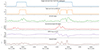 |
Figure 2 Model output (high-precision mode), target variable (derived from catalogue), and time series of some of the physical drivers for 11–15 March 2022. |
As discussed in Section 2.6, based on the PR-curve (Fig. 3), we can identify three operational regimes of the model, which single out:
A high-precision mode (red), achieving 80% precision without sacrificing too much sensitivity (i.e., predicting no less than one in three actual events) – this is obtained with a decision threshold at 0.85.
A balanced mode (orange), offering a versatile solution that works in a variety of situations, but neither markedly precise nor sensitive – this is obtained with a decision threshold at 0.68.
A high-sensitivity mode (blue), achieving 60% recall without totally compromising the precision of the model (i.e., at least one in two predicted events occurring) – this is obtained with a decision threshold at 0.54.
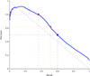 |
Figure 3 PR-curve of the model (blue line). Dots identify high-precision (red), balanced (orange), and high-sensitivity (blue) modes. |
However, before we can make any use of the model, a validation step is imperative. Validation of an ML model is a governance procedure to ensure the model produces adequate results for its data, by both quantitative and qualitative goals. This step includes testing of the model’s soundness and fit for scientific purposes, including identification of potential risks and limitations. Also, validating a classification model with imbalanced training data requires special attention to ensure that the model’s performance is correctly evaluated.
The validation framework we employed includes a global evaluation and interpretation step (Sect. 3.1) based on SHAP values and confusion matrices, then a metrics evaluation phase (Sect. 3.2), based on precision, recall, and F1-score, as introduced in Section 2.4. Moreover, the model’s performance will also be assessed by considering specific case events for which we can compare the output of the model with independent methods for identifying LSTIDs (Sect. 3.3).
3.1 Global validation and interpretation
We performed a preliminary validation of the model, evaluating the confusion matrices corresponding to the three operating modes, as discussed in Sections 2.4 and 2.6. The matrices reported in Figure 4 are normalised by rows. The balanced mode (Fig. 4a) correctly identifies 51.3% of the LSTIDs reported in the HF-INT catalogue, while ensuring a moderate incidence of false positives, amounting to 4.5% of the non-LSTID events.
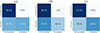 |
Figure 4 Confusion matrices for the balanced (a), high-precision (b) and high-sensitivity (c) modes; matrices are normalised by rows. |
The high-precision mode (Fig. 4b) correctly identifies 36.1% of the reported LSTIDs, while ensuring a low incidence of false positives, amounting to 1.3% of the non-LSTID events.
Lastly, the high-sensitivity mode (Fig. 4c) correctly identifies 60.0% of the reported LSTIDs, but this comes at the cost of a more pronounced incidence of false positives, amounting to 8.6% of the non-LSTID events.
Beyond that, the SHAP formalism, introduced in Section 2.5, helps us understand the model’s decision-making process and validate its operation from a physical point of view.
The beeswarm plot in Figure 5 visualises the distribution of SHAP values of the first 12 most important features. On the horizontal axis, dots represent SHAP values of individual data instances, providing crucial information about feature influence on the model output. A wider spread or higher density of dots indicates more significant variability or a more substantial impact on the predictions. The colour mapping on the vertical axis represents low or high values of the respective features, helping in identifying patterns and trends in the distribution of feature values across instances. Features are ranked by importance, allowing one to check that the model is drawing information from the physical drivers one would expect to be most impactful.
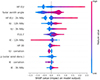 |
Figure 5 Beeswarm plot of the first 12 features ranked by importance. |
To summarise the entire distribution of SHAP values for each feature, Figure 6 is plotted. This chart lets us evaluate whether the features considered most relevant by the model align with physical arguments; indeed, it shows the mean absolute value of each feature over all instances, which is an effective way to create a global measure of feature importance. Among the most impactful variables (on average) on the model’s decisions, we find the HF-INTEU index, solar zenith angle, auroral electrojet indices, and solar radio flux. This confirms that geomagnetic and solar activity comprise the main drivers of LSTIDs.
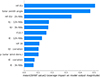 |
Figure 6 Feature importance as the average impact on model output. |
The picture returned by the model using XAI methods is non-trivial, especially given the non-linear nature of the phenomenon and the model itself. As such, the SHAP formalism proves to be an important tool in debugging ML methods with sensible domain knowledge – i.e., known physics principles.
3.2 Classification performance
As described in Section 4.1, the way to use and evaluate the model in a way that best suits the needs of the specific user is through probabilistic forecasting, which, however, requires, among other things, a precise quantification of the monetary impacts of false positives and false negatives. In the absence of such specific cost estimates, the user can rely on the three operating modes discussed in Sections 2.6 and 3.1, depending on whether they are more interested in mitigating:
Alert fatigue (high-precision mode).
An overly conservative estimate of the LSTID onset time (high-sensitivity mode).
Both of the above (balanced mode).
The cross-validated performance of the three modes in terms of Precision, equation (2), Recall, equation (3), and F1-score, equation (4), is reported in Table 3.
Precision, recall, and F1-score for the positive class of the three operating modes.
The analysis of these metrics shows that:
In high-precision mode (decision threshold set to 0.85), the model has a low false-positive rate, but reports slightly more than one in three alerts, having to be reasonable confidence in its prediction.
In high-sensitivity mode (decision threshold set to 0.54), the model correctly identifies 60% of the total alerts to be actually issued, but one in two alerts is a false positive.
In balanced mode (decision threshold set to 0.68), the performance of the model is somewhere between the other modes, identifying a somewhat cost-agnostic model.
As a baseline to interpret the goodness of metrics in Table 3, we can consider a naïve, rule-based model: if the HF-INTEU index rises above 1.75, the model predicts the occurrence of an LSTID in the next 3 h; no LSTIDs are predicted otherwise. This very simple model achieves a precision of 0.79 and a recall of 0.17, thus a F1-score of 0.29. Precision is quite high since the catalogue is a human-validated version of the HF-INTEU index; however, recall is very low (only one in six predicted events occurs), thus pushing the F1-score down. It becomes apparent how the model trades precision for recall, yielding a F1-score gain ranging from +72% to +93%, depending on the operating mode.
3.3 Event-level validation and interpretation
Breaking down model outputs into true positive and true negative, and false positive and false negative, assumes that the ground truth is known without uncertainty. This is, however, not the case, since discrepancies between the model prediction of an LSTID and the unreported occurrence of events, as well as the unreported occurrence of physical drivers along with a positive prediction and an actual occurrence of an event, might occur. In this section, we take an in-depth look at three events (listed in Table 4), which fall outside the model’s training period, to investigate the reasons behind any discrepancy between the model’s prediction and the HF-INT catalogue, or their possible agreement based on independent LSTID detection techniques. These events were chosen to analyse different situations: event 1 was not predicted by all three operating modes; event 2 was predicted with satisfactory advance under all modes; event 3 was predicted under all modes, although it was not annotated as an LSTID in the HF-INT catalogue. Since the structure of the analysis is identical for the three events, we will analyse event 1 in the following: the analyses of events 2 and 3 can be found in the Supplementary Materials.
Events considered for extensive validation of the model; tick marks indicate the presence of the event in the catalogue, of physical drivers supporting the geomagnetic nature of the event, as well as its prediction under the three operating modes.
Event 1
This event took place on December 1, 2021. The model outputs are shown in Figure 7, along with the target derived from the catalogue (the onset time is anticipated by 3 h), and some of the physical drivers – HF-INTEU, SMR, and IU indices – that summarise the geomagnetic conditions over the European continent. We note that the event is detected by the balanced and high-sensitivity operating modes, yet not by the high-precision mode. Additionally, we observe that in this case, the model is not fully capable of providing sufficient early warning in comparison to the target.
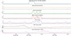 |
Figure 7 Time series of the target variable (derived from the catalogue), model outputs and main physical drivers associated with event 1. |
We can use the SHAP framework to interpret the model’s decision-making process, as outlined in Section 2.5. At 02:00 UT (Fig. 8a), the model returns a score of 0.24, as it relies on low values of the 3-hour MAV of the IU index and observes stationarity in the time series of this driver; it also finds a low HF-INTEU value. The situation changes at 03:30 UT (Fig. 8b), the onset time of the ionospheric disturbance according to the catalogue, when the model, driven primarily by HF-INTEU and the solar zenith angle, assigns a score of 0.78 to the occurrence of an LSTID. This value is sufficient to produce an alert in the balanced and high-sensitivity modes; however, the confidence is not enough for the high-precision mode. Half an hour later (Fig. 8c), the model produces a score of 0.85, which is exactly on the decision threshold of the high-precision mode. In this case, what holds the model’s confidence is essentially the stationarity of the IU index and the moderate value of its 3-hour MAV. The agreement during these hours is good with the HF-INT method (Fig. 9). The dTEC keogram (Fig. 10) shows LSTID signatures in the early morning hours (04 UT – 07 UT), albeit not very strong. A LSTID activity has also been detected by the HF-TID method for the Průhonice–Juliusruh radio link (Fig. 11). A TID with a moderate-to-strong amplitude disturbance above 40% after 1 UT on 1 December has been detected with a two-phase different propagation direction of the TID (North–West and East), both calculated with confidence precision and provided with a smooth transition. Unfortunately, further monitoring of this event was interrupted at 5 UT due to the occurrence of a negative ionospheric storm, causing a depression of the Maximum Useable Frequency (MUF) of the D2D link. MUF depressions are a well-known problem for HF communications, causing substandard quality and additional variability of propagation close to MUF (Kauristie et al., 2021). The iso-density and iso-height plots (Fig. 12) measured at Ebro Observatory digisonde (EB040) show clear LSTIDs between 01:00 UT and 06:00 UT on 1 December. Athens digisonde (AT138) reports also LSTID signatures around the same time interval. However, the LSTID signatures begin to appear one hour later at AT138. At Dourbes digisonde (DB049), there is a clear LSTID signature between 00:00 UT and 07:00 UT.
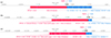 |
Figure 8 SHAP force plot for (a) 01/12/2021, 02:00 UT; (b) 01/12/2021, 03:30 UT; (c) 01/12/2021, 04:00 UT. |
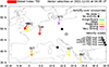 |
Figure 9 Representative map of LSTID activity observed by the HF-INT method for event 1. |
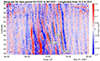 |
Figure 10 dTEC keogram for event 1. |
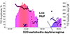 |
Figure 11 TID amplitudes and azimuth direction of propagation observed by the HF-TID method for event 1. |
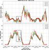 |
Figure 12 Iso-density (top panel) and iso-height (bottom panel) plots for EB040 station for event 1. Dotted rectangles indicate the occurrence of the disturbance. |
A summary view of all the detections by the different methods and the model (balanced) prediction is shown in Figure 13.
 |
Figure 13 Timeline chart showing model’s balanced output (blue), HF-INT catalogue entry (yellow) used as a ground truth, and detection by independent methods (orange) for event 1. |
4 Towards operability
In view of future implementations of the model for real-time operations in space weather services and its registration in the e-Science Centre of PITHIA-NRF (Belehaki et al., 2024), we contextualise its operability within a cost-sensitive learning framework. We also report on the possibility of operating in a probabilistic prediction mode, and state-of-the-art performance-centric monitoring strategies for covariate and concept drift, along with model updating via online learning strategies.
4.1 Cost-sensitive learning
As described in Section 2.6, the model can operate in three modes. The choice of a mode should be based on the relative cost of false positives and false negatives, which depends on the end-user requirements. In our context, a false positive means that the algorithm predicts an LSTID within 3 h, but there will be no real LSTID activity; this implies that the user is alerted unnecessarily, perhaps resulting in alert fatigue. On the other hand, a false negative implies a failure to act by the user.
To correctly assess the benefit of using our model or to select an operation mode, we should evaluate the cost of operations for an LSTID alert and tie each output to an economic value. Suppose a€ is the monetary cost of operations for an LSTID alert, while  identifies the cost of a missed alert. The total cost can be expressed as (Fernández et al., 2018)
 (9)
(9)
since the cost associated with true positives TN is zero, and the total cost may at best tend to the monetary cost of operations if only true positives occur.
Estimating a€ and  is not trivial and should be based on expert judgement, yet it is fundamental when operating in the probabilistic forecasting regime described in Section 2.6. Clearly, these estimates are beyond the scope of this work and pertain to the individual use cases.
4.2 Model calibration and uncertainty quantification
As we mentioned in Section 2.6, classification is a post hoc decision layer on top of a probabilistic prediction, thus, it involves making a definitive decision, which can be applied incorrectly. From the point of view of cost-sensitive decisions (see Sect. 4.1), calibrated class probabilities are essential. However, classifiers do not yield class probabilities in general: at best, they offer classification scores that approximate true probabilities (Johansson & Gabrielsson, 2019). In potentially high-risk settings, such miscalibrations can become hazardous and invalidate the decision-making process. However, incorporating a calibration phase, one can output not only calibrated probability estimates, but also a measure of confidence in these estimates, leading to conceivably safer outcomes.
The reliability plot of the uncalibrated model is reported in Figure 14, where the horizontal axis reports the predicted probability, while the vertical axis shows the observed relative frequency of an event.
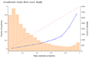 |
Figure 14 Reliability diagram of the uncalibrated model. The histogram shows the distribution of predicted probabilities, indicating the number of samples for each probability range (0.05 wide); the dashed line represents perfect reliability, while the dotted line shows the actual calibration curve, illustrating how predicted probabilities correspond to true outcomes. |
It becomes apparent how the uncalibrated model shows a significant imbalance from the point of view of the positive class. For instance, a predicted mean probability of 0.75 corresponds to an actual fraction of positives of only 30% (instead of 75%). In general, the model tends to strongly overestimate the probability of occurrence of LSTIDs, especially in the range of estimated probabilities between 0.1 and 0.9 (approximately). The achieved Brier score is 0.120.
Following the calibration methods discussed in Section 2.6, we observe how the model becomes substantially more conservative in its probability forecasts, yielding a histogram for the fraction of positives which suggests the presence of events with low, medium, and high probability of occurrence (Fig. 15).
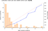 |
Figure 15 Reliability diagram of the model after Venn-ABERS calibration. Refer to caption in Figure 14 for details. |
The Brier score achieved after Venn-ABERS calibration is 0.078. The calibration is far from perfect, but the model exhibits a more predictable and safe behaviour.
Finally, Figure 16 shows the evolution over time of the predicted probabilities of an LSTID occurrence. As an example, the plot displays an interval of 8 days (9–17 March 2022). At the bottom of the plot, a red line shows the width of the prediction interval (grey band).
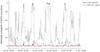 |
Figure 16 Estimated probability of LSTID occurrence for 9–17 May 2022, along with uncertainty quantification. |
It is interesting to comment on the spikes of the width of the prediction interval in light of the operation of Venn predictors. These are indeed allowed to announce several probability distributions as their prediction: when the upper and lower bounds of such a multi-probability prediction are not close to each other, one may be in a situation of Knightean uncertainty – a risk that cannot be modelled through conventional risk measurement models – and the multi-probability prediction may be considered as a useful warning (Vovk et al., 2022).
As a final point, once probabilities have been obtained following a calibration procedure, in analogy to the concepts of equation (9), the classifier could then directly minimise the expected risk (Khan et al., 2017),
 (10)
(10)
Here j is the class prediction made by the classifier; ξjk denotes the misclassification cost of classifying an instance belonging to class j into a different one – in other words, it is an estimate of the costs associated with false positives and false negatives; P(k|x) is the probability over all possible classes, given an input instance x. Thus, minimising the function in equation (10) allows one to obtain a model that fits the specific needs of the end user, even if these are not constant, but may vary over time: having estimated the probabilities P(k|x), the expected risk R(j|x) follows from the cost matrix ξ.
4.3 Performance-centric monitoring
When an ML model runs in real time, it constantly receives new data to make predictions upon; however, this data might have a different probability distribution than the one the model was trained on. Using the original model with the new data distribution can eventually cause a drop in model performance. To avoid this degradation, it is important to monitor changes in model’s performance.
Models, in general, operate on two kinds of data: features, X and targets, Y. The data shift in its most generic form can be described as a change in the joint distribution P(X, Y) of features and targets, which can be written as
 (11)
(11)
This joint distribution can vary for four independent reasons (Moreno-Torres et al., 2012):
P(X) changes, i.e., the distribution of model inputs changes – we talk about covariate shift.
P(Y) changes, i.e., the output distribution changes – we talk about a label shift.
P(Y|X) changes, i.e., for specific inputs, the distribution of the output has changed, meaning that the concept learnt during training has since then changed in the real world – we talk about a concept shift.
P(X|Y) changes, i.e., same target values manifest themselves differently in the input distribution – we talk about a manifestation shift.
Out of the four types of shifts, covariate and concept shifts are the major concerns for ML models serving predictions in production.
If the problem is covariate shift, either the decision function (like changing the threshold to make a positive prediction) or the downstream processes need to be adjusted. Importantly, simple retraining is not going to help if the data drifted to a region where it is harder to make predictions: for example, the data might concentrate closer to the class boundary for the binary classifier. As long as there is no significant concept drift, the retrained model will not learn anything new.
If the problem relates to data quality, it should be resolved upstream. Indeed, blindly retraining the model might have undesirable consequences, as the model may capture spurious patterns that only exist in bad-quality data, resulting in a less stable and worse-performing model.
If the problem is a concept shift, we envision two solutions:
Online learning, meaning that the model stays updated irrespective of any changes that might occur. If one observes that the model is regularly drifting, it might be decided to partially re-train the model as new data enters the system.
Fully retrain the model.
Once issues are solved, one can go back to monitoring the model’s performance.
5 Conclusions
In this work, we have presented an ML model capable of working on the time series of physical drivers of LSTIDs. This model, trained on a catalogue compiled by ionosphere scientists, can predict with a certain reliability the occurrence of this class of ionospheric disturbances over the European continent within a 3-hour time horizon. However, other time horizons could be explored in future work to further expand the model’s applicability. The key aspects of our research are as follows:
Although the model was trained on a catalogue of LSTID that does not resolve geographical details and built from a detection method that has inherent limitations, the performance achieved is promising: depending on the operating mode, we report a maximum precision of 0.80 or a maximum recall of 0.60, i.e. a F1-score between 0.50 and 0.56. We are not aware of other models applied to a similar problem; hence, our benchmark is a simple rule-based model derived from HF-INTEU, which reports an F1-score of 0.29.
Individual metrics cannot provide a holistic view of a model’s potential and limitations, so the validation phase relied on different analyses and comparisons with other independent methods. Also, the SHAP explanatory framework allows for analysing the decision-making process to i) interpret the model, ii) debug it (from the developer’s point of view), and iii) increase confidence in the end-user.
The model remains relevant in different scenarios through the three operating modes proposed. However, when accurate estimates of the costs associated with misclassifications are available, the model may operate in probabilistic forecasting mode, directly estimating the probability of an LSTID occurrence based on the given inputs. To fully address the potentially high-risk setting related to the effects of LSTIDs, it becomes paramount to produce reliable estimates of these probabilities. Conformal prediction and its methods allow an efficient calibration of these estimates, which are then ready to model the complex phenomena for decision making.
The methodology presented in this research offers substantial implications for space weather forecasting. By enhancing our ability to predict LSTID events and mitigate their effects, our findings can contribute to the advancement of predictive modelling capabilities and crucially, support decision-making processes in critical operational contexts.
Acknowledgments
Authors are grateful to Simone Porreca for the valuable discussions about physical modelling based on Artificial Intelligence. The editor thanks Liu Peng and two anonymous reviewers for their assistance in evaluating this paper.
Funding
The T-FORS project (https://t-fors.eu/) is funded by the European Union (GA-101081835).
Data availability statement
Aurolal electrojet data were provided by the FMI-managed IMAGE Network. The solar radio flux data were retrieved from NOAA. Solar wind and interplanetary magnetic field were sourced from NASA OMNIWeb. SMR and Newell indices were provided by SuperMAG. The Hp30 index was gathered from GFZ Potsdam. SEC, azimuth, velocity of perturbations, and the HF-INTEU index were retrieved from TechTIDE.
The HF-INT LSTID catalogue is available at the CORA repository (Segarra et al., 2024). The preprocessed data required to reproduce the above findings are available to download from: https://github.com/viventriglia/t-fors/blob/main/data/out/df_dataset.pickle. Python code and its documentation are available at the following GitHub repository: https://github.com/viventriglia/t-fors/.
Supplementary materials
Supplementary file supplied by the authors. Access Supplementary Material
References
- Afraimovich, EL, Kosogorov EA, Leonovich LA, Palamartchouk KS, Perevalova NP, Pirog OM. 2000. Determining parameters of large-scale traveling ionospheric disturbances of auroral origin using GPS-arrays. Atmos. Solar Terr. Phys. 62: 553–565. https://doi.org/10.1016/S1364-6826(00)00011-0. [CrossRef] [Google Scholar]
- Afraimovich, E, Astafyeva E, Demyanov V, Edemskiy I, Gavrilyuk N, et al. 2013. A review of GPS/GLONASS studies of the ionospheric response to natural and anthropogenic processes and phenomena. J Space Weather Space Clim 3: A27. https://doi.org/10.1051/swsc/2013049. [CrossRef] [EDP Sciences] [Google Scholar]
- Akiba, T, Sano S, Yanase T, Ohta T, Koyama M. 2019. Optuna: A next-generation hyperparameter optimization framework. In: KDD '19: Proceedings of the 25th ACM SIGKDD International Conference on Knowledge Discovery & Data Mining, pp. 2623–2631. https://doi.org/10.1145/3292500.3330701. [CrossRef] [Google Scholar]
- Altadill, D, Segarra A, Blanch E, Juan JM, Paznukhov V, Buresova D, Galkin I, Reinisch BW, Belehaki A. 2020. A method for real-time identification and tracking of traveling ionospheric disturbances using ionosonde data: First results. J Space Weather Space Clim 10: 2. https://doi.org/10.1051/swsc/2019042. [CrossRef] [EDP Sciences] [Google Scholar]
- Asamoah EN, Cafaro M, Epicoco I, Franceschi GD, Cesaroni C. 2024. A stacked machine learning model for the vertical total electron content forecasting. Adv Space Res 74(1):223–242. https://doi.org/10.1016/j.asr.2024.04.055. [CrossRef] [Google Scholar]
- Azeem I, Yue J, Hoffmann L, Miller SD, Straka III WCCrowley G. 2015.Multisensor profiling of a concentric gravity wave event propagating from the troposphere to the ionosphere. Geophys Res Lett 42(19):7874–7880. https://doi.org/10.1002/2015GL065903. [CrossRef] [Google Scholar]
- Banks, PM. 1977. Observations of joule and particle heating in the auroral zone. J Atmos Terr Phys 39: 179–193. https://doi.org/10.1016/0021-9169(77)90112-X. [CrossRef] [Google Scholar]
- Bartels, J, Heck NH, Johnston HF. 1939. The three-hour-range index measuring geomagnetic activity. Terr Magn Atmos Electric 44: 4. https://doi.org/10.1029/TE044i004p00411. [Google Scholar]
- Belehaki, A, Tsagouri I, Altadill D, Blanch E, Borries C, et al. 2020. An overview of methodologies for real-time detection, characterisation and tracking of traveling ionospheric disturbances developed in the TechTIDE project. J Space Weather Space Clim 10: 42. https://doi.org/10.1051/swsc/2020043. [CrossRef] [EDP Sciences] [Google Scholar]
- Belehaki, A, Häggström I, Kiss T, Galkin I, Tjulin A, et al. 2024. Integrating plasmasphere, ionosphere and thermosphere observations and models into a standardised open access research environment: The PITHIA-NRF international project. Adv Space Res 75: 3082–3114. https://doi.org/10.1016/j.asr.2024.11.065. [Google Scholar]
- Bergin A, Chapman SC, Gjerloev JW. 2020..AE, DST, and their SuperMAG counterparts: the effect of improved spatial resolution in geomagnetic indices. J Geophys Res Space Phys 125(5): e2020JA027828. https://doi.org/10.1029/2020JA027828. [CrossRef] [Google Scholar]
- Borries, C, Jakowski N, Wilken V. 2009. Storm induced large scale TIDs observed in GPS derived TEC. 592. Ann Geophys 27: 1605–1612. https://doi.org/10.5194/angeo-27-1605-2009. [CrossRef] [Google Scholar]
- Bowman, GG. 1965. Travelling disturbances associated with ionospheric storms. J Atmos Terr Phys 27: 1247–1261. https://doi.org/10.1016/0021-9169(65)90085-1. [CrossRef] [Google Scholar]
- Buresova, D, Belehaki A, Tsagouri I, Watermann J, Galkin I, et al. 2019. Report on methodology for the specification of TID drivers. https://doi.org/10.5281/zenodo.2555119. [Google Scholar]
- Camporeale E. 2019. The challenge of machine learning in space weather: nowcasting and forecasting. Space Weather 17(8):1166–1207. https://doi.org/10.1029/2018SW002061. [CrossRef] [Google Scholar]
- Cesaroni, C, Spogli L, Aragon-Angel A, Fiocca M, Dear V, De Franceschi G, Romano V. 2020. Neural network-based model for global Total Electron Content forecasting. J Space Weather Space Clim 10: 11. https://doi.org/10.1051/swsc/2020013. [CrossRef] [EDP Sciences] [Google Scholar]
- Chan, KL, Villard OG, Jr. 1962. Observation of large-scale traveling ionospheric disturbances by spaced-path high-frequency instantaneous-frequency measurements. J Geophys Res 67: 973–988. https://doi.org/10.1029/JZ067i003p009733. [CrossRef] [Google Scholar]
- Davis, MJ. 1971. On polar substorms as the source of large-scale traveling ionospheric disturbances. J Geophys Res 76: 4525–4533. https://doi.org/10.1029/JA076i019p04525. [CrossRef] [Google Scholar]
- Dorogush, AV, Ershov V, Gulin A. 2018. CatBoost: gradient boosting with categorical features support. ML Systems, NeurIPS 2017. https://doi.org/10.48550/arXiv.1810.11363. [Google Scholar]
- Eather, RH, Mende SB, Judge RJR. 1976. Plasma Injection at synchronous orbit and spatial and temporal auroral morphology. J Geophys Res 81 (16): 2805–2824. https://doi.org/10.1029/JA081i016p02805. [CrossRef] [Google Scholar]
- Fernández, A, García S, Galar M, Prati RC, Krawczyk B, Herrera F. 2018. Learning from imbalanced data sets. Springer International Publishing. Switzerland. ISBN: 978–3319980737. [CrossRef] [Google Scholar]
- Filho, TS, Song H, Perello-Nieto M, Santos-Rodriguez R, Kull M, Flach P. 2023. Classifier Calibration: A survey on how to assess and improve predicted class probabilities. Mach Learn 112 (9): 3211–3260. https://doi.org/10.1007/s10994-023-06336-7. [CrossRef] [Google Scholar]
- Filjar, R. 2021. A contribution to short-term rapidly developing geomagnetic storm classification for GNSS ionosphere effects mitigation model development. In: 2021 Seventh International Conference on Aerospace Science and Engineering (ICASE), Islamabad, Pakistan, pp. 1–6. https://doi.org/10.1109/ICASE54940.2021.9904168. [Google Scholar]
- Georges, TM. 1968. HF Doppler studies of traveling ionospheric disturbances. J Atmos Terr Phys 30: 735–746. https://doi.org/10.1016/S0021-9169(68)80029-7. [CrossRef] [Google Scholar]
- Guerra, M, Cesaroni C, Ravanelli M, Spogli L. 2024. Travelling Ionospheric Disturbances detection: a statistical study of detrending techniques, induced period error and near real-time observables. J Space Weather Space Clim 14: 17. https://doi.org/10.1051/swsc/2024017. [CrossRef] [EDP Sciences] [Google Scholar]
- Habarulema, JB, Katamzi ZT, Yizengaw E. 2015. First observations of poleward large-scale traveling ionospheric disturbances over the African sector during geomagnetic storm conditions. J Geophys Res Space Phys 120: 6914–6929. https://doi.org/10.1002/2015JA021066. [CrossRef] [Google Scholar]
- Habarulema, JB, Katamzi ZT, Yizengaw E, Yamazaki Y, Seemala G. 2016. Simultaneous storm time equatorward and poleward large‐scale TIDs on a global scale. Geophys Res Lett 43 (13): 6678–6686. https://doi.org/10.1002/2016GL069740. [CrossRef] [Google Scholar]
- Haralambous, H, M Guerra, J Chum, TG Verhulst, V Barta, et al. 2023. Multi‐instrument observations of various ionospheric disturbances caused by the 6 February 2023 Turkey earthquake. J Geophys Res Space Phys 128 (12): e2023JA031691. https://doi.org/10.1029/2023JA031691. [CrossRef] [Google Scholar]
- Hines, CO. 1960. Internal atmospheric gravity waves at ionospheric heights. Can J Phys 38: 1441–1481. https://doi.org/10.1139/p60-150. [CrossRef] [Google Scholar]
- Huang X, Reinisch BW, Sales GS, Paznukhov VV, Galkin IA. 2016. Comparing TID simulations using 3-D ray tracing and mirror reflection. Radio Sci 51(4): 337–343. https://doi.org/10.1002/2015RS005872. [CrossRef] [Google Scholar]
- Hunsucker RD. 1982. Atmospheric gravity waves generated in the high-latitude ionosphere: A review. Rev Geophys 20: 293–315. https://doi.org/10.1029/RG020i002p00293. [CrossRef] [Google Scholar]
- Iban MC, Şentürk E. 2022. Machine learning regression models for prediction of multiple ionospheric parameters. Adv Space Res 69(3): 1319–1334. https://doi.org/10.1016/j.asr.2021.11.026. [CrossRef] [Google Scholar]
- Johansson, U, Gabrielsson P. 2019. Are traditional neural networks well-calibrated? In: 2019 International Joint Conference on Neural Networks (IJCNN), Budapest, Hungary, pp. 1–8, https://doi.org/10.1109/IJCNN.2019.8851962. [Google Scholar]
- Jonah, OF, Zhang S, Coster AJ, Goncharenko LP, Erickson PJ, Rideout W, de Paula ER, de Jesus R. 2020. Understanding inter-hemispheric traveling ionospheric disturbances and their mechanisms. Rem Sens 12 (2): 228. https://doi.org/10.3390/rs12020228. [CrossRef] [Google Scholar]
- Kamide Y, Akasofu S-I. 1983. Notes on the auroral electrojet indices. Rev Geophys 21(7): 1647–1656. https://doi.org/10.1029/RG021i007p01647. [CrossRef] [Google Scholar]
- Kauristie, K, Morschhauser A, Olsen N, Finlay CC, McPherron RL, Gjerloev JW, Opgenoorth HJ. 2017. On the usage of geomagnetic indices for data selection in internal field modelling. Space Sci Rev 206: 61–90. https://doi.org/10.1007/s11214-016-0301-0. [CrossRef] [Google Scholar]
- Kauristie, K, Andries J, Beck P, Berdermann J, Berghmans D, et al. 2021. Space weather services for civil aviation – challenges and solutions, Rem Sens, 13 (18): 3685. https://doi.org/10.3390/rs13183685. [CrossRef] [Google Scholar]
- Khan, SH, Hayat M, Bennamoun M, Sohel F, Togneri R. 2017. Cost-sensitive learning of deep feature representations from imbalanced data. IEEE Trans Neural Netw Learn Syst 29: 3573–3587. https://doi.org/10.1109/TNNLS.2017.2732482. [Google Scholar]
- Krzysztofowicz, R. 2024. Probabilistic forecasts and optimal decisions. John Wiley & Sons Ltd, UK. [CrossRef] [Google Scholar]
- Li H, Wang C, Kan JR. 2011. Contribution of the partial ring current to the SYMH index during magnetic storms. J Geophys Res Space Phys 116(A11). https://doi.org/10.1029/2011JA016886. [Google Scholar]
- Liu, L, Zou S, Yao Y, Wang Z. 2020. Forecasting global ionospheric TEC using deep learning approach. Space Weather 18: e2020SW002501. [CrossRef] [Google Scholar]
- Liu, P, Yokoyama T, Fu W, Yamamoto M. 2022. Statistical analysis of medium-scale traveling ionospheric disturbances over japan based on deep learning instance segmentation. Space Weather 20: e2022SW003151. https://doi.org/10.1029/2022SW003151. [CrossRef] [Google Scholar]
- Lundberg, S, Lee S-I. 2017. A unified approach to interpreting model predictions. In: NIPS’17: Proceedings of the 31st International Conference on Neural Information Processing Systems. https://dl.acm.org/doi/10.5555/3295222.3295230. [Google Scholar]
- Maeda, S, Handa S. 1980. Transmission of large-scale TIDs in the ionospheric F2 region. J Atmos Terr Phys 42: 853–859. https://doi.org/10.1016/0021-9169(80)90089-6. [CrossRef] [Google Scholar]
- Makela, JJ, Otsuka Y. 2012. Overview of nighttime ionospheric instabilities at low- and mid-latitudes: coupling aspects resulting in structuring at the mesoscale. Space Sci Rev 168, 419–440. https://doi.org/10.1007/s11214-011-9816-6. [CrossRef] [Google Scholar]
- McGranaghan RM, Mannucci AJ, Wilson B, Mattmann CA, Chadwick R. 2018. New capabilities for prediction of high-latitude ionospheric scintillation: a novel approach with machine learning. Space Weather 16(11): 1817–1846. https://doi.org/10.1029/2018SW002018. [CrossRef] [Google Scholar]
- Moreno-Torres, JG, Raeder T, Alaiz-Rodriguez R, Chawla NV, Herrera F. 2012. A unifying view on dataset shift in classification. Pattern Recogn (Elsevier) 45 (1): 521–530. https://doi.org/10.1016/j.patcog.2011.06.019. [CrossRef] [Google Scholar]
- Newell PT, Gjerloev JW. 2012. SuperMAG-based partial ring current indices. J Geophys Res Space Phys 117(A5). https://doi.org/10.1029/2012JA017586. [Google Scholar]
- Ngwira, CM, Habarulema JB, Astafyeva E, Yizengaw E, Jonah OF, et al. 2019. Dynamic response of ionospheric plasma density to the geomagnetic storm of 22‐23 June 2015. J Geophys Res Space Phys 124 (8): 7123–7139. https://doi.org/10.1029/2018JA026172. [CrossRef] [Google Scholar]
- Nykiel, G, Ferreira A, Günzkofer F, Iochem P, Tasnim S, Sato H. 2024. Large‐scale traveling ionospheric disturbances over the European sector during the geomagnetic storm on March 23–24, 2023: Energy deposition in the source regions and the propagation characteristics. J Geophys Res Space Phys 129: e2023JA032145. https://doi.org/10.1029/2023JA032145. [CrossRef] [Google Scholar]
- Oyama, S, Watkins B. 2012. Generation of atmospheric gravity waves in the polar thermosphere in response to auroral activity. Space Sci Rev 168 (1–4): 463–473. https://doi.org/10.1007/s11214-011-9847-z. [CrossRef] [Google Scholar]
- Paznukhov VV, Galushko VG, Reinisch BW. 2012. Digisonde observations of TIDs with frequency and angular sounding technique. Adv Space Res 49(4): 700–710. https://doi.org/10.1016/j.asr.2011.11.012. [CrossRef] [Google Scholar]
- Poniatowski, M, Nykiel G. 2020. Degradation of kinematic ppp of GNSS stations in central europe caused by medium-scale traveling ionospheric disturbances during the St. Patrick’s day 2015 geomagnetic storm. Rem Sens 12: 1–15, https://doi.org/10.3390/rs12213582. [Google Scholar]
- Reinisch B, Galkin I, Belehaki A, Paznukhov V, Huang X, Altadill D, et al. 2018. Pilot ionosonde network for identification of traveling ionospheric disturbances. Radio Sci 53(3): 365–378. https://doi.org/10.1002/2017RS006263. [CrossRef] [Google Scholar]
- Saito, A, Fukao S, Miyazaki S. 1998. High resolution mapping of TEC perturbations with the GSI GPS network over Japan. Geophys Res Lett 25: 3079–3082. https://doi.org/10.1029/98GL52361. [CrossRef] [Google Scholar]
- Savastano G, Komjathy A, Verkhoglyadova O, Mazzoni A, Crespi M, Wei Y, Mannucci AJ. 2017. Real-time detection of tsunami ionospheric disturbances with a stand-alone GNSS receiver: a preliminary feasibility demonstration. Sci Rep 7. https://doi.org/10.1038/srep46607. [CrossRef] [Google Scholar]
- Segarra, A, Altadill D, de Paula V, Navas-Portella V. 2024. Catalogue LSTID. CORA Repositori de Dades de Recerca, V1, https://doi.org/10.34810/data1383. [Google Scholar]
- Tanskanen EI. 2009. A comprehensive high-throughput analysis of substorms observed by IMAGE magnetometer network: Years 1993–2003 examined. J Geophys Res Space Phys 114(A5). https://doi.org/10.1029/2008JA013682. [CrossRef] [Google Scholar]
- Tapping, KF. 2013. The 10.7 cm solar radio flux (F10.7). Space Weather 11: 7. https://doi.org/10.1002/swe.20064. [Google Scholar]
- Timoté, CC, Juan JM, Sanz J, González-Casado G, Rovira-Garciá A, Escudero M. 2020. Impact of medium-scale traveling ionospheric disturbances on network real-time kinematic services: CATNET study case. J Space Weather Space Clim 10: 29. https://doi.org/10.1051/swsc/2020030. [CrossRef] [EDP Sciences] [Google Scholar]
- Tsugawa, T, Saito A, Otsuka Y, Yamamoto M. 2003. Damping of large-scale traveling ionospheric disturbances detected with GPS networks during the geomagnetic storm. J Geophys Res 108: 1127. https://doi.org/10.1029/2002JA009433. [CrossRef] [Google Scholar]
- Themens DR, Watson C, Žagar N, Vasylkevych S, Elvidge S, McCaffrey A, et al. 2022. Global propagation of ionospheric disturbances associated with the 2022 Tonga volcanic eruption. Geophys Res Lett 49(7): e2022GL098158. https://doi.org/10.1029/2022GL098158. [CrossRef] [Google Scholar]
- Verhulst, TGW, Altadill D, Barta V, Belehaki A, Burešová D, et al. 2022. Multi-instrument detection in Europe of ionospheric disturbances caused by the 15 January 2022 eruption of the Hunga volcano. J Space Weather Space Clim 12: 35. https://doi.org/10.1051/swsc/2022032. [CrossRef] [EDP Sciences] [Google Scholar]
- Vovk, V, Gammerman A, Shafer G. 2022. Probabilistic classification: Venn predictors. Algorithmic learning in a random world. Springer Nature Switzerland AG. https://doi.org/10.1007/978-3-031-06649-8. [CrossRef] [Google Scholar]
- Vovk, V, Petej I. 2014. Uncertainty in artificial intelligence. In: Proceedings of the 30th Conference. , AUAI Press. ISBN 978-0974903910, https://doi.org/10.48550/arXiv.1211.0025. [Google Scholar]
- Watanabe, S. 2023. Tree-structured Parzen estimator: understanding its algorithm components and their roles for better empirical performance. https://doi.org/10.48550/arXiv.2304.11127. [Google Scholar]
- Yamazaki Y, Matzka J, Stolle C, Kervalishvili G, Rauberg J, Bronkalla O, et al. 2022. Geomagnetic Activity Index Hpo. Geophys Res Lett 49(10): e2022GL098860. https://doi.org/10.1029/2022GL098860. [CrossRef] [Google Scholar]
- Zakharenkova, I, Astafyeva E, Cherniak I. 2016. GPS and GLONASS observations of large-scale traveling ionospheric disturbances during the 2015 St. Patrick’s Day storm, J Geophys Res Space Phys 121: 12138–12156. https://doi.org/10.1002/2016JA023332. [CrossRef] [Google Scholar]
- Zhou, C, Zhao Z, Yang G, Chen G, Hu Y, Zhang Y. 2012. Evidence of low‐latitude daytime large‐scale traveling ionospheric disturbances observed by high‐frequency multistatic backscatter sounding system during a geomagnetically quiet period. J Geophys Res Space Phys 117: A6. https://doi.org/10.1029/2012JA017605. [Google Scholar]
Cite this article as: Ventriglia V, Guerra M, Cesaroni C, Spogli L, Altadill D, et al. 2025. An explainable machine learning model for largescale travelling ionospheric disturbances forecasting. J. Space Weather Space Clim. 15, 25. https://doi.org/10.1051/swsc/2025020.
All Tables
Precision, recall, and F1-score for the positive class of the three operating modes.
Events considered for extensive validation of the model; tick marks indicate the presence of the event in the catalogue, of physical drivers supporting the geomagnetic nature of the event, as well as its prediction under the three operating modes.
All Figures
|
Figure 1 CatBoost working principle, which learns subsequent trees to reduce the error made by the previous ones, thus minimizing the loss function in equation (1). |
| In the text | |
|
Figure 2 Model output (high-precision mode), target variable (derived from catalogue), and time series of some of the physical drivers for 11–15 March 2022. |
| In the text | |
|
Figure 3 PR-curve of the model (blue line). Dots identify high-precision (red), balanced (orange), and high-sensitivity (blue) modes. |
| In the text | |
|
Figure 4 Confusion matrices for the balanced (a), high-precision (b) and high-sensitivity (c) modes; matrices are normalised by rows. |
| In the text | |
|
Figure 5 Beeswarm plot of the first 12 features ranked by importance. |
| In the text | |
|
Figure 6 Feature importance as the average impact on model output. |
| In the text | |
|
Figure 7 Time series of the target variable (derived from the catalogue), model outputs and main physical drivers associated with event 1. |
| In the text | |
|
Figure 8 SHAP force plot for (a) 01/12/2021, 02:00 UT; (b) 01/12/2021, 03:30 UT; (c) 01/12/2021, 04:00 UT. |
| In the text | |
|
Figure 9 Representative map of LSTID activity observed by the HF-INT method for event 1. |
| In the text | |
|
Figure 10 dTEC keogram for event 1. |
| In the text | |
|
Figure 11 TID amplitudes and azimuth direction of propagation observed by the HF-TID method for event 1. |
| In the text | |
|
Figure 12 Iso-density (top panel) and iso-height (bottom panel) plots for EB040 station for event 1. Dotted rectangles indicate the occurrence of the disturbance. |
| In the text | |
|
Figure 13 Timeline chart showing model’s balanced output (blue), HF-INT catalogue entry (yellow) used as a ground truth, and detection by independent methods (orange) for event 1. |
| In the text | |
|
Figure 14 Reliability diagram of the uncalibrated model. The histogram shows the distribution of predicted probabilities, indicating the number of samples for each probability range (0.05 wide); the dashed line represents perfect reliability, while the dotted line shows the actual calibration curve, illustrating how predicted probabilities correspond to true outcomes. |
| In the text | |
|
Figure 15 Reliability diagram of the model after Venn-ABERS calibration. Refer to caption in Figure 14 for details. |
| In the text | |
|
Figure 16 Estimated probability of LSTID occurrence for 9–17 May 2022, along with uncertainty quantification. |
| In the text | |
Current usage metrics show cumulative count of Article Views (full-text article views including HTML views, PDF and ePub downloads, according to the available data) and Abstracts Views on Vision4Press platform.
Data correspond to usage on the plateform after 2015. The current usage metrics is available 48-96 hours after online publication and is updated daily on week days.
Initial download of the metrics may take a while.