© British Geological Survey, UKRI, Published by EDP Sciences 2026

1 Introduction

The Swarm mission, launched in November 2013, consists of three identical satellites in near-polar orbits, dedicated to measuring the Earth’s magnetic field with very high accuracy. Two satellites orbit at a lower altitude in close proximity, while the third orbits at a higher altitude, producing a steady drift both in the local time at the orbits’ ascending nodes and in the separation between the orbits’ ascending nodes. This unique configuration allows for a wide range of new models to be developed for the various sources of the magnetic field, from the core to the magnetosphere (e.g. Olsen and Stolle 2017). In this study, we develop an algorithm to construct a Model of the Magnetosphere (MMA) for the night-side, using data from Swarm satellites. On the night side, the ionospheric fields are relatively weak and lack the complex dynamics observed on the day side, allowing empirical models to represent these fields accurately. This, in turn, enables a more reliable representation of the MMA, where the ionospheric influence can be removed effectively. The use of only Swarm satellites allows us to use a complete, high-quality database with a span of more than 10 years. The development and validation of this algorithm will also enable the future integration of additional data sources (such as platform magnetometers), as well as offer users a degree of customisation in producing night-side magnetospheric models using the VirEs virtual environment (Smith et al. 2022). One of the drawbacks of our Swarm-only model is its limited local time coverage, which greatly restricts the resolution of the model’s meridional features. We expect that climatological analysis helps mitigate these issues, by using data from varying orbital configurations throughout the whole mission.

The magnetic field measured at spacecraft altitudes results from a combination of various sources. The strongest component comes from the geodynamo. Earth’s outer core consists of metallic liquid that flows slowly, generating a self-sustained magnetic field. In addition, there is a broad array of natural magnetic field sources that influence the geomagnetic field across a wide range of frequencies (Constable and Constable 2023). When the electrically-charged solar wind reaches Earth, its interaction with the main field creates a shock wave centred at the subsolar point. The majority of the plasma flows around Earth, but the Earth’s magnetic field lines undergo deformation, resulting in what is known as the magnetosphere. This has an asymmetric shape due to compression on the sun-facing direction by flow towards Earth and extension on the night side.

Various other current systems exist within Earth’s geomagnetic environment, shaped by the interaction between the interplanetary magnetic field and the core field. The magnetosphere is asymmetric with respect to the day-night plane, resulting in daily variations (Ganushkina et al. 2018). The geomagnetic field also exhibits seasonal variations due to the inclination of the Earth’s rotation axis relative to the ecliptic plane. Additionally, it undergoes decadal variations correlated with the solar cycle; i.e., the Sun’s activity follows an approximately 11- and 22-year cycle, and this variation is observed on Earth.

Space weather thus refers to variations in the external field (to Earth’s surface) on the scale of days to weeks, driven by solar wind conditions. In contrast, space climate encompasses variations driven by solar wind conditions over longer time scales, such as months to years. These variations are governed by the Earth-Sun system’s geometry, which results in an annual periodicity. Additionally, geomagnetic activity is influenced by the solar cycle, as solar maxima increase the likelihood of enhanced geomagnetic activity due to a greater number of coronal mass ejections (CMEs).

Earth’s magnetic environment contains a network of interconnected currents, including the ring current (RC), a large-scale toroidal current in the equatorial plane extending from roughly 3 to 8 Earth radii (Chapman and Ferraro 1941). During geomagnetically quiet times, the ring current is mostly symmetric around Earth, with some day-to-night structure (e.g., Ganushkina et al. 2018). This simplicity allows the RC to be effectively modelled as a dipole magnetic source. However, studies of the ring current have found not only day-night asymmetries within the ring current, but also dusk-dawn asymmetries (e.g., Ohtani 2021), some of which are prevalent during geomagnetic storms.

During periods of disturbance, plasma is injected and transported from the night-side plasma sheet to the inner magnetosphere. This process creates a highly asymmetric plasma pressure distribution in the inner magnetosphere, which is reflected in the spatial asymmetry of the ring current in the dawn-dusk direction (Ganushkina et al. 2018).

A complex system of currents links the polar regions to the equatorially distributed plasma and forms part of the partial westward ring current. Shore et al. (2017) identify the main modes governing the behaviour observed during geomagnetically active periods. Their analysis revealed that the DP1 and DP2 current systems (the substorm and eastward auroral electrojets) account for a significant portion of the variations detected on the ground. The latter contributes to the development of the storm-time ring current in the inner magnetosphere, indicating that the high-latitude ionosphere interacts with the ring current region through magnetic field lines.

During geomagnetic storms, particles are transported from the magnetotail through the inner magnetosphere to the day-side magnetopause. This process leads to a surge in the partial ring current, which intensifies predominantly on the night-side and develops additional non-dipolar structures (e.g., Ohtani 2021; Ganushkina et al. 2018; Moore 2007; Lockwood et al. 2020). In extreme cases, natural variations in the external magnetic field at Earth’s surface may reach up to 10% of the internal field strength and can induce large ground-level electric fields, which may affect human technology and infrastructure (Pulkkinen et al. 2005; Svalgaard and Hansen 2013).

One commonly used measure of geomagnetic disturbance is known as the Dst index (e.g. Nose et al. 2015), which is computed using the horizontal component of the magnetic field measured at four mid-latitude ground observatories. After removing secular, seasonal, and daily variations, a latitude-weighted average across all local times is computed, yielding a measure of variations in the strength of the horizontal magnetic field at the equator. Negative values of this index correlate with a stronger ring current in the magnetosphere, making it a reliable indicator of geomagnetic storm intensity. Measurements equivalent to the Dst index but with minute-resolution data are also available, such as SYM-H.

The SYM-H index is used to describe axisymmetric geomagnetic disturbances at mid-latitudes in the horizontal component (H) (e.g. Imajo et al. 2022; Bower et al. 2025). The Dst index uses ground observatory data, recorded with high precision and available in real time. However, definitive values differ from preliminary as jumps in measurement baselines can affect the calculated indices, sometimes rendering them unreliable for characterising the geomagnetic field.

In recent decades, improved coverage has been achieved by spacecraft measurements (e.g., Reigber et al. 2002; Olsen et al. 2003; Friis-Christensen et al. 2008). Unlike observatory-based measurements, polar-orbiting satellite observations offer almost complete geographic coverage. Due to their position, particularly their altitude, magnetic measurements taken in space exhibit different sensitivities to various sources of magnetic fields compared to ground-based observatories. For instance, satellites in low Earth orbit are closer to magnetospheric currents, but they are also positioned above ionospheric current systems. Therefore, it is necessary to develop algorithms that can separate these sources to effectively combine satellite and observatory data during joint analysis.

Efforts to investigate the magnetospheric field using satellite data have been undertaken in previous studies. For instance, Maus and Lühr (2005) and Lühr and Maus (2010) utilised data from Ørsted and CHAMP to construct a model of the quiet-time magnetosphere. Their findings indicate that variations in the magnetospheric field are primarily governed by two contributions: (1) a set of coefficients in Solar Magnetic (SM) coordinates, parameterised by the E_st and I_st indices; and (2) a set of coefficients in Geocentric Solar Magnetic (GSM) coordinates, parameterised by the B_y component of the Interplanetary Magnetic Field (IMF), which lies perpendicular to the Earth–Sun line within the ecliptic plane. The authors attribute the SM contribution to the influence of the equatorial ring current, RC, and the Chapman-Ferraro currents. The GSM component is predominantly driven by tail currents.

Various models of the magnetospheric fields from spacecraft measurements are available, including a comprehensive model built from satellite and ground observatories measurements (Sabaka et al. 2020), as well as a dedicated fast-track Swarm-only model produced daily (Hamilton 2013). More recently, Fillion et al. (2023) developed a model of the near-Earth magnetic field from inner magnetospheric currents. Their study presents a 25-year model (1997–2022) of hourly variations in the near-Earth inner magnetospheric field, validated against the RC index (Olsen et al. 2014). The model captures local-time asymmetries and performs best at degree 2 for moderate to high geomagnetic activity. Ou et al. (2024) developed a magnetospheric model incorporating data from the Macao Science Satellite-1 (MSS–1A) and Swarm missions. Their findings confirm that the dawn-dusk asymmetry, previously observed during geomagnetic storms, persists during both geomagnetically quiet periods and the storm recovery phase. They propose that local time asymmetry is a key factor in the evolution of the ring current, significantly affecting plasma injection and decay processes within the magnetosphere.

Additionally, there are magnetospheric models based on the analysis of observatory and spacecraft measurements (e.g. Finlay et al. 2020). There are also a variety of empirical models of how the magnetosphere responds to given solar wind conditions, some global (e.g Tsyganenko 2002a, 2002b; Tsyganenko and Sitnov 2005), some focused on specific phenomena or regions (e.g. Antonova and Stepanova 2021). In order to understand the behaviour of the ring current, we need a global model that includes the night-side magnetospheric currents.

Tsyganenko (2002a) built a global semi-empirical model that uses solar wind conditions from in-situ measurements, and a field deformation technique accounting for various asymmetries observed in the ring current. This model has been adapted to other planets (e.g., Korth et al. 2015; Tsyganenko and Andreeva 2014) by adding or excluding several features as needed. This model can account for a ring current that is asymmetric both in local time and latitude (Tsyganenko and Sitnov 2007). Modelling the detailed magnetospheric environment is challenging due to its complexity and non-linear dynamics, and there are still many issues to be addressed (e.g., Borovsky 2022). For example, Castillo et al. (2017) studied how well the Tsyganenko and Sitnov (2005) reproduced the transient magnetospheric signal measured at four mid-latitude stations in the Northern Hemisphere. They found that with this empirical approach, the East-West component is more accurate than the North-South component, especially on geomagnetically active days, where the symmetric and partial ring currents dominate the variability and magnitude of the field at the Earth’s surface. Even under the best conditions, remaining discrepancies–particularly in North-South direction–arise, likely from the geometry and variation in the field-aligned currents.

Magnetic measurements on a spacecraft in low Earth orbit are primarily influenced by the core, crustal magnetisation, ionosphere, and magnetic fields created by magnetospheric currents. Depending on the relative position between the source of the magnetic field and the measuring spacecraft, we can define them to have an internal or external origin. At Earth’s surface, the rapidly varying internal component is driven by currents induced by the external component. Consequently, changes in the external magnetic potential must always precede the response of the internal magnetic field. The conductivity distribution governs the surface induction response. A frequency-dependent response coefficient can be constructed to separate the inducing and induced components of a measured field. This coefficient is determined by the mantle’s electrical conductivity. Based on this principle, an approach can be developed that relies on the inversion of electromagnetic transfer functions, organised as the Q-response matrix. This matrix links the external (inducing) and internal (induced) coefficients in a spherical harmonic expansion of the time-dependent magnetic field originating from the magnetosphere (Olsen 1999; Grayver et al. 2021).

In this paper, we employ a technique that enables magnetic field solution for both the zonal and meridional components of the magnetospheric field (see Grayver et al. 2021). We provide a brief description of the methodology used, along with the data and models applied to calculate the residuals we processed (see Sect. 2). Additionally, we compare our results with previously published magnetospheric models during the St. Patrick’s Storm in March 2015 (e.g. Kader et al. 2022).

Using our inversion technique, we analyse the temporal and spatial behaviour of the magnetosphere based on Swarm spacecraft measurements from launch (November 2013) to the present. Our focus is on the night-side magnetosphere, where we observe seasonal variations during geomagnetically quiet periods (see Sect. 3.5). We acknowledge that correctly resolving degree and order 3 features is not always possible given the configuration of the satellites during the mission, so the study is also curiosity driven in order to examine the limitations. This is obvious in storm scenarios with very rapid field changes.

In Section 3.6, we examine the solar cycle variability of the MMA. Furthermore, we investigate local-time and latitudinal variations during geomagnetic storms by developing a model that integrates Swarm and MSS–1A spacecraft data. This combined model demonstrates significant improvements due to enhanced local time coverage during the ‘Gannon’ geomagnetic storm (10–11 May 2024) in Section 3.7. Finally, we evaluate the validity of our new model, highlight its advantages, and discuss future developments and improvements to the algorithm in Section 4.

2 Methodology

We use the spacecraft measurements in geocentric coordinates (GEOC) and models of the core, crustal, and ionospheric fields (these models will be discussed below) to produce a residual where we expect the signal of magnetospheric origin is present. There are two parts to this signal: the primary field that comes from the magnetosphere (inducing), and a secondary signal generated by the magnetospheric field inducing currents in the Earth’s mantle (induced). From the frame of reference of the spacecraft, the inducing field is external, and the induced field is internal.

In order to separate external and internal sources from the satellite measured magnetic fields, we use the Q-matrices (Olsen 1999). The residuals that correspond to the magnetospheric field can be expressed in the frequency domain, $\overrightarrow{B}(\overrightarrow{r},\omega )$, where $\overrightarrow{r}=(r,\theta ,\varphi )$, and ω refers to the signal frequency from a Fourier transform applied to the signal time series. Assuming the magnetic field is potential, i.e., there are no currents at satellite altitude, one can write

$$\begin{array}{c}\hfill \overrightarrow{B}(\overrightarrow{r},\omega )=-\mathrm{\nabla }{V}^e(\overrightarrow{r},\omega )-\mathrm{\nabla }{V}^i(\overrightarrow{r},\omega ),\end{array}$$(1)

where each of the potentials may be expanded in spherical harmonics as

$$\begin{array}{c}\hfill V^e(\overrightarrow{r},\omega )=a\sum _{n=1}^N\sum _{m=-n}^n{ϵ}_n^m(\omega ){\left(\frac{r}{a}\right)}^n{P}_n^m(cos\theta )e^{\mathrm{im}\varphi },\end{array}$$(2)

and

$$\begin{array}{c}\hfill V^i(\overrightarrow{r},\omega )=a\sum _{n=1}^N\sum _{m=-n}^n{\iota }_n^m(\omega ){\left(\frac{a}{r}\right)}^{n+1}{P}_n^m(cos\theta )e^{\mathrm{im}\varphi },\end{array}$$(3)

where a is Earth’s radius, P_n ^m is the Legendre polynomial degree n and order m, ϵ_n ^m and ι_n ^m are the external and internal coefficients, respectively.

The internal field arises from the induction of the external part on the conducting crust, sea, and mantle. The relationship between the inducing and induced fields depends on the electrical conductivity σ. We can use the Fourier domain representation and we write the conductivity as a function of frequency, σ(ω). Each external coefficient ϵ_n ^m induces the internal coefficient ι_n ^m .

Assuming that horizontal variations in crustal and upper mantle conductivity are small (i.e., ∂σ/∂x, ∂σ/∂y ≪ σ/p with p as the skin depth), it is possible to estimate the amplitude and phase response to an electromagnetic impulse such as

$$\begin{array}{c}\hfill {\iota }_n^m(\omega ,\sigma )=Q_n(\omega ,\sigma ){ϵ}_n^m(\omega ),\end{array}$$(4)

where Q_n(ω, σ) is the Q-matrix transfer function.

The ratio of induced to inducing field can be measured and it depends exclusively on the Earth’s conductivity depth profile, σ(r). From Grayver et al. (2021), it is possible to write the external coefficients by minimising the difference between the observed horizontal field, $B_{\alpha i}$, and the modelled horizontal fields $B_{n\alpha }^m({\overrightarrow{r}}_i,t,\sigma )$, where α denotes the horizontal field components θ and ϕ. Here, ${\overrightarrow{r}}_i$ and t represent the position and time of the ith measured vector B_{α i}.

$$\begin{array}{cc}& B_{n\theta }^m({\overrightarrow{r}}_i,t,\sigma )=\sum _{j=0}^{N_t}-I_{Q_n}(j,\sigma ){\left(\frac{a}{r_i}\right)}^{n+2}{\frac{\mathrm{d}{P}_n^m(cos\theta )}{\mathrm{d}\theta }|}_{\theta ={\theta }_i}\hfill \\ \hfill & \times [q_n^m(t-j\mathrm{\Delta }t)cos(m{\varphi }_i)+s_n^m(t-j\mathrm{\Delta }t)sin(m{\varphi }_i)]\hfill \end{array}$$(5)

$$\begin{array}{cc}& B_{n\varphi }^m({\overrightarrow{r}}_i,t,\sigma )=\sum _{j=0}^{N_t}{I}_{Q_n}(j,\sigma ){\left(\frac{a}{r_i}\right)}^{n+2}\frac{m}{sin{\theta }_i}{P}_n^m(cos{\theta }_i)\hfill \\ \hfill & \times [q_n^m(t-j\mathrm{\Delta }t)sin(m{\varphi }_i)-s_n^m(t-j\mathrm{\Delta }t)cos(m{\varphi }_i)]\hfill \end{array}$$(6)

where $N_t=\frac{T}{\mathrm{\Delta }\mathrm{t}}$ represents the total time span of the samples T divided by the time interval window Δt. The function $I_{{\mathrm{Qn}}_{}}(j,\sigma )={\int }_{j\mathrm{\Delta t}-\mathrm{\Delta t}/2}^{j\mathrm{\Delta t}+\mathrm{\Delta t}/2}{\mathrm{Qn}}_{}(t,\sigma )\mathrm{dt}$ is the time-domain representation of the Q-matrix transfer functions, ${\mathrm{qnm}}_{}^{}$ and ${\mathrm{snm}}_{}^{}$ are the Gauss coefficients for the external field (see Grayver et al. 2021).

This solution assumes that magnetic field sources (i.e., the magnetospheric field sources) remain constant over the time interval Δt. However, for a rapidly varying magnetospheric configuration, this approximation provides only a time-averaged source field. To ensure sufficient geographical coverage, we use long-period (6 h–12 h) cadences for Δt. This approximation is reasonably well justified even in an active geomagnetic environment because the long-timescale asymmetry in the configuration of the ring current is expected.

We have implemented this algorithm using two of the Swarm satellites, enabling simultaneous coverage of two local times for most of the observation period. We use data from Swarm Alpha (A) and Bravo (B). Since Swarm B orbits at a higher altitude, it drifts through local time at a different rate compared to the lower pair (A/C). During certain periods, such as immediately after launch and in 2021, the satellites were in approximately the same local time, limiting the measurement of higher-order terms.

We start with Level 1b data from the Swarm satellites A and B in the NEC frame. We subsample the data at a 15-second cadence. To apply the above decomposition, it is essential to remove all non-magnetospheric fields. We use standard Swarm-derived models for the core, crustal, and ionospheric fields to compute the residuals required for our Model of the Magnetosphere (MMA). During the preparation of this study, we tested various model combinations. Our analysis shows that the choice of ionospheric model introduces only minor differences in the resulting magnetospheric models. The results presented in this paper are based on the dedicated models from the Swarm Level 2 products (e.g. Beggan et al. 2013). Following Hamilton (2013), we use the core and crustal models from the dedicated core model: MCO_SHA_2D (Rother et al. 2013) for the core and MLI_SHA_2D (Thébault et al. 2013) for the lithosphere; in combination with the ionospheric model CM4 (for a more recent version, CM6, see Sabaka et al. 2020).

For performance assessment and comparison, we also cross-checked the results with models available from the VirES for Swarm service, such as the CHAOS Core (Finlay et al. 2020) and CHAOS Static (Olsen et al. 2006) models, as well as the ionospheric dedicated model MIO_SHA_2D (Chulliat et al. 2013). We find minor differences in the results depending on the integration time used for the ionospheric models. A 12-h cadence yields identical MMA model results, while 8-h and 6-h cadences show deviations of up to 10 nT during geomagnetically active periods.

Using the core, crust, and ionospheric models, we subtract their estimates from the Swarm data to compute residuals which we assume contain primarily the magnetospheric contribution. We select only night-side data, i.e., measurements between 18:00 and 06:00 local time. High geomagnetic latitudes are excluded, and only measurements below |60^°| dipole latitude are considered. After computing the residuals, the algorithm fits data within a time window Δt, assuming that the sources remain constant and stationary. This allows for the separation of internal and external components, where the external component corresponds to the magnetosphere model.

This algorithm finds the best-fit coefficients for a spherical harmonic representation of the Gauss coefficients to degree and order 3 for inducing and induced fields, assuming the sources are stationary. The MMA model consists of time series of the inducing spherical harmonic coefficients, which give a 2D representation of the external fields at spacecraft altitude as measured by the Swarm satellites.

It is important to note that, due to the data selection we chose, i.e., night-time data only, our solution does not have any input information to resolve the coefficients q_l ^2p + 1 (i.e., when the order m = 2p + 1 is odd) in SM coordinates. These values are, as expected, close to zero, but we have not used this as a constraint in the MMA solution.

3 Results

In this section, we demonstrate how the MMA performs by comparing it with previous models based on satellite data (Sect. 3.2) and ground observatory data (Sect. 3.4). We use the MMA to observe the evolution of the night-side magnetosphere during the March 2015 (St. Patricks Day) storm (Sect. 3.3). We also include results of the climatological evolution of the night-side magnetosphere in Sections 3.5 and 3.6.

3.1 Evaluation of the model using satellite residuals

Using the algorithm presented in the previous section, we are able to reproduce the magnetic field measured by the Swarm satellites.

Based on the time interval used to define the model, we calculate the modelled field at the interpolated satellite positions, resulting in the horizontal field evaluated with a Δt cadence. To compare with the magnetospheric residual, we resample the measured field to match the model’s time cadence (see Fig. 1).

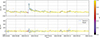Figure 1. Plots of the time series of the residual magnetospheric field measured by Swarm A during the St Patrick storm 2015. The light blue line shows the satellite interpolated measurements at the modelled time, and the colour dots show the model evaluated at the interpolated satellite positions. The colours indicate the coefficient of determination, R2, for the model linear regression fit to the Gauss coefficients. Colour values close to 1 (yellow) indicate a good linear fit to the time interval chosen for the model (8 h in this case) and values close to zero (dark purple) indicate that the fit is not good and the data variation within the time window is large.

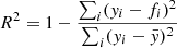
Comparing the measured and modelled horizontal components, we see a number of outliers in the model. These outliers do not always coincide with poor fits to the data, i.e., with low values of R², shown in the colour map in Figure 1. The measure for quality of the linear fit used is the coefficient of determination

$$\begin{array}{c}\hfill R^2=1-\frac{{\sum }_i{({\mathrm{yi}}_{}-{\mathrm{fi}}_{})}^2}{{\sum }_i{({\mathrm{yi}}_{}-\overline{y})}^2}\end{array}$$(7)

where y_i is the i-th measured value, $\overline{y}$ is the mean observed value over the interval Δt, and f_i is the predicted value at i (e.g. B in equations (5) and (6)). Colour values close to 1 (yellow) indicate a good linear fit to the time interval chosen for the model (8h in this case) and values close to zero (dark purple) indicate that the fit is not good and the data variation within the time window is large.

To ensure an independent comparison with the model predictions, we make use of magnetic field measurements from the MSS–1A mission, whose data are not involved in the model construction. We compared the model predictions at the MSS–1A satellite locations from January to September 2025. To derive the observed MMA at the MSS–1A positions, we applied the same filtering and smoothing procedures used for the Swarm data in Figure 1, interpolating both the satellite locations and the magnetic field measurements accordingly. The resulting residuals represent the differences between the measured and modelled MMA signals at MSS–1A throughout most of 2025. The distribution of these model–measurement differences is shown in Figure 2.

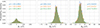Figure 2. Histograms showing the distribution of the residuals (modelled minus measured MMA) for 8-h cadence models with maximum spherical harmonic degrees lmax = 1 (blue), lmax = 2 (orange), and lmax = 3 (green). Each panel includes the mean (μ) and standard deviation of the corresponding distribution. The comparison is based on a model derived from Swarm A and B data and measurements from MSS–1A. The east–west component is the best resolved across all three models, whereas the radial component exhibits a broader spread. Overall, the integrated results show no significant differences between the three models for MSS–1A data collected from January to October 2025.

The distribution of these residuals shows that the best-resolved component overall is B_ϕ, i.e. the east-west component, with a standard deviation of approximately 10 nT. Conversely, B_r displays the largest deviation at approximately 40 nT. This behaviour is expected, as the radial component is not explicitly accounted for in our model; instead, the solution assumes it to arise from the divergence-free potential field. We do not observe major differences between the various values of l_max.

3.2 Comparison with Previous Satellite-Based Magnetospheric Models

Using a method similar to that described in Section 2, Olsen (2021) computed a model of the magnetospheric field for the period 1 March to 30 April 2015. Their study utilised data from the Swarm A and B satellites, supplemented by measurements from platform magnetometers on CryoSat-2 and GRACE (A and B). During this period, the local time coverage provided by Swarm A and B alone was limited because their orbital planes were separated by only 20° in March 2015. The results of the external field decomposition in spherical harmonics are shown in Figure 3, which presents Olsen’s model coefficients to degree and order 2 (coloured lines), the fast-track Swarm model (MMA_SHA_2F, grey) of Hamilton (2013), and our new MMA up to degree and order 3 (black).

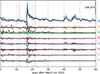Figure 3. Time series of external field spherical harmonic coefficients during March to April 2015, in geocentric coordinates. Results from Olsen (2021) are shown as coloured lines; the daily fast-track magnetospheric model from Swarm-only data, MMA_SHA_2F (grey), $q_1^0$, $q_1^1$, and $s_1^1$; and the model from this study, MMA (black). The vertical dashed lines indicate the times corresponding to the snapshots in Figure 4.

The dipole component ($q_1^0$) shows good agreement with the solution by Olsen (2021). The integration time for our model (black) in Figure 3 is 8 hours, while the fast-track model (grey) and Olsen’s model (coloured lines) use a 1.5-h sampling. As a result, finer-scale features captured in the higher time-cadence models are naturally smoothed in our solution. The storm maximum value of $q_1^0$ differs between the models presented here. These differences are influenced by the method of calculation of the residuals but mainly the chosen time interval Δt of 8 hours.

The new MMA model exhibits variations in the higher order harmonics that are not present in Olsen’s solution. This is due to differences in local time coverage. The Olsen model benefits from multiple satellites which provided a more homogeneous local time sampling, whereas our model relies on data from only two local time sectors. The local time separation of Swarm A and B was 1.5 h (about 20^°) in early 2015.

3.3 Asymmetry during 17 March 2015 storm

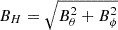
We can examine the spatial evolution of the external field during storm periods. Figure 4 presents three snapshots of the external magnetic field, showing the magnitude of the horizontal component, i.e. 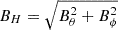${\mathrm{BH}}_{}=\sqrt{{\mathrm{B\theta }}_2^{}+{\mathrm{B\varphi }}_2^{}}$ (blue to yellow) at spacecraft altitude. These fields are drawn in solar magnetic coordinates, with midnight at the centre of each map. The shaded regions mark the day-side, where no satellite data are included, but the spherical harmonic model will nevertheless produce a value. The boundaries of this region correspond to dusk (18:00 local time) on the left and dawn (06:00 local time) on the right.

Figure 4. Snapshots of the external field calculated from Swarm satellite measurements during the St. Patrick’s storm, March 2015. The figures show the magnitude of the horizontal component ${\mathrm{BH}}_{}=\sqrt{{\mathrm{B\theta }}_2^{}+{\mathrm{B\varphi }}_2^{}}$ of the external field. Each map is in solar magnetic coordinates, with midnight at the centre. The shaded region represents the day-side.

The left panel depicts the pre-storm quiet time background field where the external field on the night-side resembles a tilted dipole. At storm maximum (middle panel), the external field intensifies significantly, exhibiting a strong non-axisymmetric component. The maximum horizontal component shifts toward dusk and south of the geomagnetic equator. Finally, during the storm recovery phase (right panel), the external field weakens but remains enhanced toward dusk.

3.4 Comparison with ground observatory models

To evaluate the magnetospheric model using ground observatory data, we compare it with the Vector Magnetic Disturbance (VMD) index (Thomson and Lesur 2007) (Fig. 5). The VMD index is derived from nighttime data collected from observatories situated at magnetic latitudes below 50^°, ensuring compatibility with the coverage of our magnetospheric model.

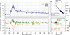Figure 5. (Left) Time series of the dipolar components of our MMA model (points) with a 12-h cadence and the Vector Magnetic Disturbance (VMD) index Thomson and Lesur (2007) (lines). The top left panel shows the axisymmetric dipole, $q_0^1$, from the MMA (blue points) alongside the symmetric part of the negative VMD index (blue line). The bottom left panel displays the equatorial dipoles $q_1^1$ (green) and $s_1^1$ (orange) from the same MMA solution (points), compared with the negative VMD index (lines). (Right) Correlation plots of MMA vs. VMD. Text boxes with the best fit line and corresponding Pearson correlation coefficient R value, using the same colours as the left panels. Dotted grey line shows a line with slope –1.

Thomson and Lesur (2007) constructed the VMD index by processing 1-minute averaged geomagnetic data obtained from INTERMAGNET observatories time-series. This index is designed to monitor rapid fluctuations in the strength and direction of large-scale external magnetic fields. It comprises two three-dimensional vector time series that cover three-month intervals throughout the year, with data from observatories situated between 50^° and −50^° magnetic latitudes, under specific local time and zenith angle conditions. The mathematical framework used to analyse the observed data incorporates constants representing linear time variations that account for slowly changing core fields, and rapid fluctuations attributed to the large-scale external field and its corresponding induced effects. The estimation process for the VMD index consists of three main steps: first, determining observatory offsets and linear trends; second, modelling rapid variations; and finally, separating external signals from internal ones.

We find good agreement between the degree l = 1 component of the MMA solution and the negative VMD index during the St. Patrick’s geomagnetic storm (17 March 2015), see Figure 5, right panels. For the VMD calculation, observatory offsets are determined such that the quiet-time mean VMD value is zero. However, for the MMA model, we explicitly include the quiet-time ring current. This methodological difference accounts for the offset observed in Figure 5 between the VMD index (lines) and MMA model (dots), seen also as a non-zero intercept on the right side correlation plots. See also the discussion on offsets with the Dst index in Grayver et al. (2021). As expected, the coefficient $q_1^1$, which is poorly resolved due to the data selection, shows no correlation with the VMD counterpart (shown in green).

3.5 Seasonal quiet time magnetosphere

The model is most effective in capturing features of the magnetosphere that persist over several days rather than rapid fluctuations during magnetic storms. We analysed the external field during geomagnetically quiet periods by computing the mean external field for each month over the 10-year duration of the Swarm mission as shown in Figure 6. The lower panel presents the 10-year average of the axisymmetric dipole during quiet days, where ${\langle q_1^0\rangle }_{\mathrm{day}}<10$ nT. Two vertical solid grey lines indicate the time of the equinoxes. We observe increased activity near the equinoxes, particularly in April and September, and lower activity during the solstices. This seasonal pattern is consistent with previous observations (e.g., Russell and McPherron 1973).

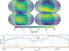Figure 6. Maps showing the magnitude of the horizontal magnetospheric field at satellite altitude. Each map represents a monthly averaged field based on geomagnetically quiet periods over the 10-year Swarm mission dataset. The panels display averages for March (upper left) and June (upper right), September (lower left) and December (lower right). The bottom panel shows the average monthly amplitude of $\langle q_1^0\rangle$ for all data over 10 years (blue) and for selected quiet time only (orange). Dashed grey vertical lines correspond to the times of the snapshots above. Solid grey vertical lines mark the equinoxes.

The top panel of Figure 6 displays maps of the horizontal component of the magnetospheric field at spacecraft altitude in solar magnetic coordinates, with midnight at the centre. The maps correspond to March, June, September, and December, representing equinoxes (left) and solstices (right). The external field remains predominantly dipolar and is strongly influenced by the ring current. The dipole appears tilted during June and December, when the Earth’s northern pole is oriented toward and away from the Sun, respectively.

This seasonal behaviour results from the change in inclination of the geomagnetic dipole relative to the Sun-Earth line (e.g., Hoshi et al. 2018; Eggington et al. 2020). The combined effect of Earth’s internal dipole tilt and inclination of the rotational axis causes Earth’s magnetic field to align with the Earth-Sun line during solstices (June and December) and to be perpendicular to it during equinoxes (March and September) (Lockwood et al. 2020). Additionally, we observe an enhancement of the field in the dusk equatorial region.

3.6 Variation over a solar cycle

From the 10 years of model evaluation, we can observe how the magnetospheric field varies with the solar cycle. Figure 7 presents the monthly means of the axisymmetric dipole ($q_1^0$) for the whole dataset (blue) and during quiet periods (orange), where days with ${\langle q_1^0\rangle }_{\mathrm{day}}<10$ nT are classified as geomagnetically quiet periods. We show the sunspot number (green dots) and the 13-month averaged sunspot number (green line) from SILSO World Data Center (2013–2025).

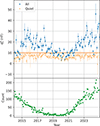Figure 7. Monthly mean values of $q_1^0$ in GEOC coordinates, for all data (blue) and for quiet days (orange). We use ${\langle q_1^0\rangle }_{\mathrm{day}}<10$ nT as the threshold for quiet days, represented by the horizontal orange line in the $q_1^0$ plot. The bottom panel shows the sunspot number (green circles) and the smoothed sunspot number (green line) from SILSO World Data Center (2013–2025).

The models indicate a background constant value of the ring current of $q_1^0\sim 8$ nT. This axisymmetric ring current is enhanced during storm periods, with both the intensity and frequency of activity increasing during solar maximum. This value is consistent with the ∼10 nT offset seen in the axisymmetric dipole, shown in blue in Figure 5, between the MMA and the VMD index.

Alternatively, we can identify active periods within this dataset. Active days are selected based on the criterion ${\langle q_1^0\rangle }_{\mathrm{day}}>50$ nT, corresponding to periods of geomagnetic storms. Figure 8 presents the monthly means of these active-day data for three Gauss coefficients: $q_1^0$, $s_1^1$, and $s_2^1$, in SM coordinates. Additionally, we include the Kernel Density Estimate, which highlights the highest occurrence of these coefficients during geomagnetic activity. Since these are monthly means, active months typically include multiple storms within the same period. Despite the large variability, positive values of $q_1^0$ are consistent with observations of depressions in the horizontal components at ground-based observatories, a feature also captured by the Dst index. Negative values of $s_1^1$, on the order of 10 nT, indicate an enhancement in the equatorial horizontal component, while non-zero values of $s_2^1$ suggest a dusk–dawn asymmetry.

Using the same dataset of active days, we transformed the data into solar magnetic coordinates. We determined the modal value of the inducing coefficients, rounded to two decimal places, and reconstructed the radial and horizontal fields corresponding to the most common inducing field, as shown in Figure 9. The typical configuration of the magnetospheric field during a geomagnetic storm is a dipolar field tilted towards dawn, with an enhanced RC near the dusk terminator. This configuration is expected to characterise the magnetosphere during the storm recovery phase, as this phase has the longest duration.

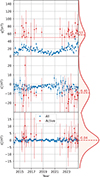Figure 8. Monthly mean values of $q_1^0$, $s_1^1$ and $s_2^1$ in SM coordinates for all data (blue) and for Active days (red). We use ${\langle q_1^0\rangle }_{\mathrm{day}}>50$ nT as the threshold for active days, represented by the horizontal red line in the $q_1^0$ plot. On the right side, using the same y-axis values, we show the Kernel Density Estimation (KDE) to find the most likely values for these three coefficients, shown in red. The highest occurrence value is shown with a horizontal dashed line and its value is given in red above the line.

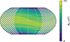Figure 9. Solar magnetic maps of the night-side were generated using the highest occurrence Gauss coefficients for active periods, as indicated by the red circles in Figure 8. The resulting configuration for active periods reveals an enhancement in the dusk region and a slightly tilted ring current (RC), which is displaced northward at the dusk terminator and southward at the dawn terminator.

3.7 Addition of MSS–1A night-side coverage

To improve local time coverage, we combine data from Swarm and MSS–1A. The MSS–1A spacecraft was launched on 21 May 2023 and has provided high-quality magnetic measurements since 2 November 2023. Unlike the Swarm constellation, MSS–1A has an orbital inclination of 41^° (e.g., Zhang 2023).

We analyse the magnetospheric model results using a combination of Swarm and MSS–1A data, comparing MMA models at various integration times. Longer integration periods of 12, 8, and 6 hours produce comparable results for the axisymmetric dipole (Fig. 10). However, a 3-h Δt cannot resolve an accurate model using Swarm data alone. This time resolution requires an improved local time coverage, only possible by incorporating MSS–1A data. This limitation likely extends to higher harmonics, though the number of available models for comparison islimited.

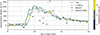Figure 10. Time series of $q_1^0$ for May 2024. Colours indicate integration time: blue (3 h), grey (6 h), and yellow (8 h). Open triangles represent results using only Swarm data, while dots show results from the combined Swarm and MSS–1A dataset. In green, we also include the negative Dst index with the dashed green line representing a 6-h moving average of the -Dst index.

4 Discussion

We constructed a new model of the night-side magnetosphere using Swarm-only data, enhancing our understanding of magnetospheric dynamics during both quiet and storm conditions. The model captures the magnetospheric field up to degree and order 3, with local time resolution constrained by the orbital configuration of the satellites, which changes during the mission due to precession. While challenges arise due to the limited local time coverage, particularly in defining meridional coefficients, the MMA remains comparable to previous models such as that of Hamilton (2013) and Olsen (2021), while extending the time series to the full operational period of the Swarm mission. However, the degree 3 and to a lesser extent degree 2 coefficients are often cross-correlated due to the generally limited local time coverage across much of the mission.

With the MMA, we can determine the geometrical configuration of the night-side magnetosphere during geomagnetic storms, enabling the direct observation of storm variability at different local times (e.g., Pinzon-Cortes et al. 2025; Lockwood et al. 2019). Even though we do not recommend using an integration time Δt of less than 6 hours for Swarm-only data, large geomagnetic storms can still be captured with the q₁⁰, and their impact could potentially be analysed in near real time using MMA with Swarm FAST data, and perhaps complementary missions to improve the local time coverage.

The seasonal variation of the quiet-time ring current has been derived, showing consistency with observations of the seasonal shifts in the magnetospheric neutral point (e.g. Eggington et al. 2020). As expected, the ring current plane shifts southward and northward along the Earth-Sun line during June and December, respectively (see Fig. 6). We observe an enhancement of the seasonal ring current due to geometric alignment, which allows for more efficient energy transfer from the solar wind into the magnetosphere during equinoxes.

Over a 10-year period, the background quiet-time ring current remains largely stable, as indicated by the orange points in Figure 7. However, during periods of heightened solar activity, characterised by an increased sunspot number (shown in green), the ring current intensifies in response to enhanced energy transfer from the interplanetary magnetic field to the magnetosphere (blue points).

Analysing the configuration of active days during the Swarm mission, we find that during geomagnetic storms, the magnetosphere is predominantly characterised by a dipolar field tilted towards the dawn terminator, with a stronger ring current near the dusk terminator (Fig. 9).

Integrating low-inclination orbital data from MSS–1A significantly improves local time coverage, greatly enhancing the inversion process for producing the MMA (Fig. 10). In the future, we anticipate further improvements with the launch of the NanoMagSat constellation (Brown et al. 2023) and additional MSS satellites.

With this model, we can provide a space-based Dst proxy by calculating $q_1^0$, with a 6-h cadence using the new FAST data from Swarm, adding to current now-cast capabilities other measurements (e.g. Orr et al. 2024. This decomposition allows for near real-time monitoring of geomagnetic storms and the tracking of asymmetries developing on the night-side during storm evolution.

5 Conclusions

A new model of the magnetosphere has been developed, based on over ten years of Swarm data from November 2013 to January 2025. The model captures the variation of the magnetosphere to degree and order 3 using night-side only measurements.

We describe the development of the model and illustrate the application to understanding of storm times, quiet periods and seasonal to solar-cycle changes in the magnetosphere. We find the steady ring current (dipole) holds steady at around 8 nT while the majority of the variation over the solar cycle relates to short periods of intense storms.

For the first time, this model offers a high-resolution representation of the nighttime magnetosphere. It can be used to compute residuals that exclude magnetospheric effects or be integrated with other measurements to improve our understanding of Earth’s magnetic field variations.

Acknowledgments

The authors thank William Brown and Callum Watson for their valuable discussions. We also extend our gratitude to Nils Olsen and Alexander Grayver for providing their data and models. We are grateful to the three anonymous reviewers for their constructive comments. This paper is published with the permission of the Executive Director of the British Geological Survey (UKRI). The editor thanks three anonymous reviewers for their assistance in evaluating this paper.

Funding

This work was funded by the European Space Agency under the DISC-5 programme.

Conflicts of interest

The authors declare no Conflict of Interest.

Data availability statement

All figures contain data from the Swarm mission courtesy of ESA. The data are publicly available at http://swarm-diss.eo.esa.int. We also extend our gratitude to the China National Space Administration (CNSA) and the Macao Special Administrative Region Government for providing data from the MSS–1A satellite mission (https://mss.must.edu.mo/index.html).

References

All Figures

Figure 1. Plots of the time series of the residual magnetospheric field measured by Swarm A during the St Patrick storm 2015. The light blue line shows the satellite interpolated measurements at the modelled time, and the colour dots show the model evaluated at the interpolated satellite positions. The colours indicate the coefficient of determination, R2, for the model linear regression fit to the Gauss coefficients. Colour values close to 1 (yellow) indicate a good linear fit to the time interval chosen for the model (8 h in this case) and values close to zero (dark purple) indicate that the fit is not good and the data variation within the time window is large.

In the text

Figure 2. Histograms showing the distribution of the residuals (modelled minus measured MMA) for 8-h cadence models with maximum spherical harmonic degrees lmax = 1 (blue), lmax = 2 (orange), and lmax = 3 (green). Each panel includes the mean (μ) and standard deviation of the corresponding distribution. The comparison is based on a model derived from Swarm A and B data and measurements from MSS–1A. The east–west component is the best resolved across all three models, whereas the radial component exhibits a broader spread. Overall, the integrated results show no significant differences between the three models for MSS–1A data collected from January to October 2025.

In the text

Figure 3. Time series of external field spherical harmonic coefficients during March to April 2015, in geocentric coordinates. Results from Olsen (2021) are shown as coloured lines; the daily fast-track magnetospheric model from Swarm-only data, MMA_SHA_2F (grey), $q_1^0$, $q_1^1$, and $s_1^1$; and the model from this study, MMA (black). The vertical dashed lines indicate the times corresponding to the snapshots in Figure 4.

In the text

Figure 4. Snapshots of the external field calculated from Swarm satellite measurements during the St. Patrick’s storm, March 2015. The figures show the magnitude of the horizontal component ${\mathrm{BH}}_{}=\sqrt{{\mathrm{B\theta }}_2^{}+{\mathrm{B\varphi }}_2^{}}$ of the external field. Each map is in solar magnetic coordinates, with midnight at the centre. The shaded region represents the day-side.

In the text

Figure 5. (Left) Time series of the dipolar components of our MMA model (points) with a 12-h cadence and the Vector Magnetic Disturbance (VMD) index Thomson and Lesur (2007) (lines). The top left panel shows the axisymmetric dipole, $q_0^1$, from the MMA (blue points) alongside the symmetric part of the negative VMD index (blue line). The bottom left panel displays the equatorial dipoles $q_1^1$ (green) and $s_1^1$ (orange) from the same MMA solution (points), compared with the negative VMD index (lines). (Right) Correlation plots of MMA vs. VMD. Text boxes with the best fit line and corresponding Pearson correlation coefficient R value, using the same colours as the left panels. Dotted grey line shows a line with slope –1.

In the text

Figure 6. Maps showing the magnitude of the horizontal magnetospheric field at satellite altitude. Each map represents a monthly averaged field based on geomagnetically quiet periods over the 10-year Swarm mission dataset. The panels display averages for March (upper left) and June (upper right), September (lower left) and December (lower right). The bottom panel shows the average monthly amplitude of $\langle q_1^0\rangle$ for all data over 10 years (blue) and for selected quiet time only (orange). Dashed grey vertical lines correspond to the times of the snapshots above. Solid grey vertical lines mark the equinoxes.

In the text

Figure 7. Monthly mean values of $q_1^0$ in GEOC coordinates, for all data (blue) and for quiet days (orange). We use ${\langle q_1^0\rangle }_{\mathrm{day}}<10$ nT as the threshold for quiet days, represented by the horizontal orange line in the $q_1^0$ plot. The bottom panel shows the sunspot number (green circles) and the smoothed sunspot number (green line) from SILSO World Data Center (2013–2025).

In the text

Figure 8. Monthly mean values of $q_1^0$, $s_1^1$ and $s_2^1$ in SM coordinates for all data (blue) and for Active days (red). We use ${\langle q_1^0\rangle }_{\mathrm{day}}>50$ nT as the threshold for active days, represented by the horizontal red line in the $q_1^0$ plot. On the right side, using the same y-axis values, we show the Kernel Density Estimation (KDE) to find the most likely values for these three coefficients, shown in red. The highest occurrence value is shown with a horizontal dashed line and its value is given in red above the line.

In the text

	Figure 9. Solar magnetic maps of the night-side were generated using the highest occurrence Gauss coefficients for active periods, as indicated by the red circles in Figure 8. The resulting configuration for active periods reveals an enhancement in the dusk region and a slightly tilted ring current (RC), which is displaced northward at the dusk terminator and southward at the dawn terminator.
In the text

	Figure 10. Time series of $q_1^0$ for May 2024. Colours indicate integration time: blue (3 h), grey (6 h), and yellow (8 h). Open triangles represent results using only Swarm data, while dots show results from the combined Swarm and MSS–1A dataset. In green, we also include the negative Dst index with the dashed green line representing a 6-h moving average of the -Dst index.
In the text

References

- Antonova, EE and Stepanova MV. 2021. The impact of turbulence on physics of the geomagnetic tail. Front Astron Space Sci 8:26. https://doi.org/10.3389/FSPAS.2021.622570/BIBTEX. [Google Scholar]
- Beggan, CD, Macmillan S, Hamilton B, and Thomson AW. 2013. Independent validation of Swarm Level 2 magnetic field products and ‘Quick Look’ for Level 1b data. Earth Planets Space 65:1345–1353. https://doi.org/10.5047/EPS.2013.08.004. [Google Scholar]
- Borovsky, JE. 2022. Grand challenge for space physics. Front Astron Space Sciences 9:855060. https://doi.org/10.3389/FSPAS.2022.855060/BIBTEX. [Google Scholar]
- Bower, GE, Milan, SE, Imber S, Schillings A, Fleetham A, Beggan C, and Gjerloev, JW. 2025. Asymmetry in the ring current during geomagnetic disturbances. J Geophys Res Space Phys 130(3):e2024JA033492. https://doi.org/10.1029/2024JA033492. [Google Scholar]
- Brown W, Gómez Pérez N, Beggan C, Hammer M, Finlay C, and Hulot G. 2023. The potential of geomagnetic virtual observatories with NanoMagSat. In: Proceedings XXVIII General Assembly of the International Union of Geodesy and Geophysics (IUGG) https://doi.org/10.57757/IUGG23-3072. [Google Scholar]
- Castillo Y, Pais MA, Fernandes J, Ribeiro P, Morozova AL, and Pinheiro FJ. 2017. Geomagnetic activity at Northern Hemisphere’s mid-latitude ground stations: How much can be explained using TS05 model. J Atmos Sol-Terr Phys, 165-166:38–53. https://doi.org/10.1016/j.jastp.2017.11.002. [Google Scholar]
- Chapman S., and Ferraro VCA. 1941. The geomagnetic ring-current: its radial stability. Terres Magn Atmos Electricity, 46(1):1–6. https://doi.org/10.1029/TE046i001p00001. [Google Scholar]
- Chulliat A, Vigneron P, Thébault E, Sirol O, and Hulot G. 2013. Swarm SCARF dedicated ionospheric field inversion chain. Earth Planets Space 65:1271–1283. https://doi.org/10.5047/eps.2013.08.006. [Google Scholar]
- Constable C, and Constable S. 2023. A grand spectrum of the geomagnetic field. Phys Earth Planet Inter 344:107090. https://doi.org/10.1016/j.pepi.2023.107090, https://www.sciencedirect.com/science/article/pii/S0031920123001164. [Google Scholar]
- Eggington JW, Eastwood JP, Mejnertsen L, Desai RT, and Chittenden JP. 2020. Dipole Tilt Effect on Magnetopause Reconnection and the Steady-State Magnetosphere-Ionosphere System: Global MHD Simulations. J Geophys Res Space Phys 125:e2019JA027510. https://doi.org/10.1029/2019JA027510. [Google Scholar]
- Fillion M, Chulliat A, Alken P, Kruglyakov M, and Kuvshinov A. 2023. A model of hourly variations of the near-Earth magnetic field generated in the inner magnetosphere and its induced counterpart. J Geophys Res Space Phys 128:e2023JA031913. https://doi.org/10.1029/2023JA031913. [Google Scholar]
- Finlay CC, Kloss C, Olsen N, Hammer MD, Tøffner-Clausen L, Grayver A, and Kuvshinov A. 2020. The CHAOS-7 geomagnetic field model and observed changes in the South Atlantic Anomaly. Earth Planets Space 72:156. https://doi.org/10.1186/s40623-020-01252-9. [Google Scholar]
- Friis-Christensen, E, Lühr H, Knudsen D, and Haagmans R. 2008. Swarm – An Earth Observation Mission investigating Geospace. Adv Space Res 41:210–216. https://doi.org/10.1016/J.ASR.2006.10.008. [CrossRef] [Google Scholar]
- Ganushkina NY, Liemohn MW, and Dubyagin S. 2018. Current Systems in the Earth’s Magnetosphere. Rev Geophys 56:309–332. https://doi.org/10.1002/2017RG000590. [Google Scholar]
- Grayver AV, Kuvshinov A, and Werthmüller D. 2021. Time-domain modeling of three-dimensional Earth’s and planetary electromagnetic induction effect in ground and satellite observations. J Geophys Res Space Phys 126:e2020JA028672. https://doi.org/10.1029/2020JA028672, https://onlinelibrary.wiley.com/doi/full/10.1029/2020JA028672. [Google Scholar]
- Hamilton B. 2013. Rapid modelling of the large-scale magnetospheric field from Swarm satellite data. Earth Planets Space 65:1295–1308. https://doi.org/10.5047/EPS.2013.09.003, https://earth-planets-space.springeropen.com/articles/10.5047/eps.2013.09.003. [CrossRef] [Google Scholar]
- Hoshi Y, Hasegawa H, Kitamura N, Saito Y, and Angelopoulos V. 2018. Seasonal and Solar Wind Control of the Reconnection Line Location on the Earth’s Dayside Magnetopause. J Geophys Res Space Phys 123:7498–7512. https://doi.org/10.1029/2018JA025305. [Google Scholar]
- Imajo S, Matsuoka A, Toh H, and Iyemori T. 2022. Mid-latitude Geomagnetic Indices ASY and SYM (ASY/SYM Indices). https://repository.kulib.kyoto-u.ac.jp/dspace/handle/2433/267216. [Google Scholar]
- Kader SS, Dashora N, and Niranjan K. 2022. Spatial and Temporal Confinement of the Ionospheric Responses During the St. Patrick’s Day Storm of March 2015. Space Weather 20(9):e2022SW003157, https://doi.org/10.1029/2022SW003157. [Google Scholar]
- Korth H, Tsyganenko NA, Johnson CL, Philpott LC, Anderson BJ, Asad MMA, Solomon SC, and McNutt RL. 2015. Modular model for Mercury’s magnetospheric magnetic field confined within the average observed magnetopause. J Geophys Res Space Phys 120:4503. https://doi.org/10.1002/2015JA021022 https://www.ncbi.nlm.nih.gov/pmc/articles/PMC5014231/. [Google Scholar]
- Lühr H and Maus S. 2010. Solar cycle dependence of quiet-time magnetospheric currents and a model of their near-Earth magnetic fields. Earth Planets Space 62:843–848. https://doi.org/10.5047/eps.2010.07.012. [Google Scholar]
- Lockwood M, Bentley SN, Owens MJ, Barnard LA, Scott CJ, Watt CE, Allanson O, and Freeman MP. 2019. The development of a space climatology: 3. Models of the evolution of distributions of space weather variables with timescale. Space Weather 17:180–209. https://doi.org/10.1029/2018SW002017. [Google Scholar]
- Lockwood M, Owens MJ, Barnard LA, Haines C, Scott CJ, McWilliams KA, and Coxon JC. 2020. Semi-annual, annual and Universal Time variations in the magnetosphere and in geomagnetic activity: 1. Geomagnetic data. J Space Weather Space Clim 10:23. https://doi.org/10.1051/SWSC/2020023. [CrossRef] [EDP Sciences] [Google Scholar]
- Maus S, and Lühr H. 2005. Signature of the quiet-time magnetospheric magnetic field and its electromagnetic induction in the rotating Earth. Geophys J Inter 162:755–763. https://doi.org/10.1111/J.1365-246X.2005.02691.X. [Google Scholar]
- Moore TE. 2007. Ring Current. Springer, Netherlands, Dordrecht, pp. 863–865. [Google Scholar]
- Nose M, Iyemori T, Sugiura M, and Kamei T. 2015. Geomagnetic Dst Index. https://doi.org/10.17593/14515-74000, https://isds-datadoi.nict.go.jp/wds/10.17593_14515-74000.html. [Google Scholar]
- Ohtani S. 2021. Revisiting the partial ring current model: longitudinal asymmetry of ground magnetic depression during geomagnetic storms. J Geophys Res Space Phys 126:e2021JA029643. https://doi.org/10.1029/2021JA029643. [Google Scholar]
- Olsen N. 1999. Induction studies with satellite data. Surveys Geophys 20:309–340. https://doi.org/10.1023/A:1006611303582/METRICS, https://link.springer.com/article/10.1023/A:1006611303582. [Google Scholar]
- Olsen N. 2021. Magnetometer data from the GRACE satellite duo. Earth Planets Space 73:1–20. https://doi.org/10.1186/S40623-021-01373-9, https://earth-planets-space.springeropen.com/articles/10.1186/s40623-021-01373-9. [CrossRef] [Google Scholar]
- Olsen N, Lühr H, Finlay CC, Sabaka TJ, Michaelis I, Rauberg J, and Tøffner-Clausen L. 2014. The CHAOS-4 geomagnetic field model. Geophys J Inter 197(2):815–827. https://academic.oup.com/gji/article-pdf/197/2/815/1705410/ggu033.pdf, https://doi.org/10.1093/gji/ggu033. [Google Scholar]
- Olsen N, Lühr H, Sabaka TJ, Mandea M, Rother M, Tøffner-Clausen L, and Choi S. 2006. CHAOS – A model of the Earth’s magnetic field derived from CHAMP, Ørsted, and SAC-C magnetic satellite data. Geophys J Inter 166:67–75. https://dx.doi.org/10.1111/j.1365-246X.2006.02959.x. [Google Scholar]
- Olsen N, Primdahl F, Tøffner-Clausen L, Sabaka T, Brauer P, et al. 2003. Calibration of the Ørsted vector magnetometer. Earth Planets Space 55:11–18. https://doi.org/10.1186/BF03352458/METRICS, https://earth-planets-space.springeropen.com/articles/10.1186/BF03352458. [Google Scholar]
- Olsen N, and Stolle C. 2017. Magnetic signatures of ionospheric and magnetospheric current systems during geomagnetic quiet conditions-an overview. Space Sci Rev 206:5–25. https://doi.org/10.1007/S11214-016-0279-7, https://link.springer.com/article/10.1007/s11214-016-0279-7. [CrossRef] [Google Scholar]
- Orr, L, Beggan C, and Brown W. 2024. A regional space weather hazard variation index utilising Swarm FAST data. J Space Weather Space Clim 14:30. https://doi.org/10.1051/SWSC/2024033, https://www.swsc-journal.org/articles/swsc/abs/2024/01/swsc240028/swsc240028.html. [Google Scholar]
- Ou JM, Jiang Y, and Yan Q. 2024. Study on the local time asymmetry of the Earth’s ring currents based on multiple low-Earth-orbit satellite magnetic observations. Sci China Technol Sci 67:3354–3364. https://doi.org/10.1007/S11431-023-2685-1/METRICS, https://link.springer.com/article/10.1007/s11431-023-2685-1. [Google Scholar]
- Pinzon-Cortes S, Gómez-Pérez N, and Domínguez SV. 2025. Ring current local time dependence during geomagnetic storms using equatorial Dst-proxies. Acta Geodaetica et Geophysica 60:97–114 https://doi.org/10.1007/S40328-024-00459-6, https://link.springer.com/10.1007/s40328-024-00459-6. [Google Scholar]
- Pulkkinen A, Lindahl S, Viljanen A, and Pirjola R. 2005. Geomagnetic storm of 29–31 October 2003: Geomagnetically induced currents and their relation to problems in the Swedish high-voltage power transmission system. Space Weather 3:S08C03 https://doi.org/10.1029/2004SW000123. [Google Scholar]
- Reigber C, Lühr H, and Schwintzer P. 2002. CHAMP mission status. Adv Space Res 30:129–134. https://doi.org/10.1016/S0273-1177(02)00276-4. [CrossRef] [Google Scholar]
- Rother M, Lesur V, and Schachtschneider R. 2013. An algorithm for deriving core magnetic field models from the Swarm data set. Earth Planets Space 65:1223–1231. https://doi.org/10.5047/EPS.2013.07.005, https://link.springer.com/articles/10.5047/eps.2013.07.005. [Google Scholar]
- Russell CT, and McPherron RL. 1973. Semiannual variation of geomagnetic activity. J Geophys Res 78:92–108. https://doi.org/10.1029/JA078I001P00092. [CrossRef] [Google Scholar]
- Sabaka TJ, Tøffner-Clausen L, Olsen N, and Finlay CC. 2020. CM6: a comprehensive geomagnetic field model derived from both CHAMP and Swarm satellite observations. Earth Planets Space 72:1–24. https://doi.org/10.1186/S40623-020-01210-5. [NASA ADS] [CrossRef] [Google Scholar]
- Shore RM, Freeman MP, Wild JA, and Gjerloev JW. 2017. A high-resolution model of the external and induced magnetic field at the Earth’s surface in the Northern Hemisphere. J Geophys Res Space Phys 122:2440–2454. https://doi.org/10.1002/2016JA023682. [Google Scholar]
- SILSO World Data Center. 2013–2025. The International Sunspot Number. https://www.sidc.be/SILSO/home. [Google Scholar]
- Smith ARA, Pačes M, and Swarm DISC 2022. Python tools for ESA’s Swarm mission: VirES for Swarm and surrounding ecosystem. Front Astron Space Sci 9:1002697 https://doi.org/10.3389/fspas.2022.1002697, https://www.frontiersin.org/journals/astronomy-and-space-sciences/articles/10.3389/fspas.2022.1002697. [CrossRef] [Google Scholar]
- Svalgaard L, and Hansen WW. 2013. Solar activity - past, present, future. J Space Weather Space Clim 3:A24. https://doi.org/10.1051/SWSC/2013046. [Google Scholar]
- Thébault E, Vigneron P, Maus S, Chulliat A, Sirol O, and Hulot G. 2013. Swarm SCARF dedicated lithospheric field inversion chain. Earth Planets Space 65:1257–1270. https://doi.org/10.5047/EPS.2013.07.008, https://earth-planets-space.springeropen.com/articles/10.5047/eps.2013.07.008. [Google Scholar]
- Thomson AW, and Lesur V. 2007. An improved geomagnetic data selection algorithm for global geomagnetic field modelling. Geophys J Int 169:951–963. https://dx.doi.org/10.1111/j.1365-246X.2007.03354.x. [CrossRef] [Google Scholar]
- Tsyganenko NA. 2002a. A model of the near magnetosphere with a dawn-dusk asymmetry 1. Mathematical structure. J Geophys Res Space Phys 107:SMP 12–1. https://dx.doi.org/10.1029/2001JA000219. [Google Scholar]
- Tsyganenko NA. 2002b. A model of the near magnetosphere with a dawn-dusk asymmetry 2. Parameterization and fitting to observations. J Geophys Res Space Phys 107:SMP 10–1. https://dx.doi.org/10.1029/2001JA000220. [Google Scholar]
- Tsyganenko NA and Andreeva VA. 2014. On the “bowl-shaped” deformation of planetary equatorial current sheets. Geophys Res Lett 41:1079–1084. https://dx.doi.org/10.1002/2014GL059295. [Google Scholar]
- Tsyganenko NA and Sitnov MI. 2005. Modeling the dynamics of the inner magnetosphere during strong geomagnetic storms. J Geophys Res Space Phys 110:3208. https://dx.doi.org/10.1029/2004JA010798. [Google Scholar]
- Tsyganenko NA and Sitnov MI. 2007. Magnetospheric configurations from a high-resolution data-based magnetic field model. J Geophys Res Space Phys 112:A06225 https://dx.doi.org/10.1029/2007JA012260. [Google Scholar]
- Zhang K. 2023. A novel geomagnetic satellite constellation: Science and applications. Earth Planet Phys 7(1):4–21. https://dx.doi.org/10.26464/epp2023019, https://www.eppcgs.org/en/article/doi/10.26464/epp2023019. [Google Scholar]
Cite this article as: Gómez-Pérez N. and Beggan C. D. 2026. A Swarm-only model of the magnetosphere to degree and order 3. J. Space Weather Space Clim. 16, 26. https://doi.org/10.1051/swsc/2026017.