| Issue |
J. Space Weather Space Clim.
Volume 16, 2026
Topical Issue - Space Climate: Solar Extremes, Long-Term Variability, and Impacts on Earth’s System
|
|
|---|---|---|
| Article Number | 13 | |
| Number of page(s) | 18 | |
| DOI | https://doi.org/10.1051/swsc/2026012 | |
| Published online | 07 May 2026 | |
Research Article
On stellar activity cycle-related cosmic ray modulation effects in the astrosphere of Proxima Centauri
1
Center for Space Research, North-West University, Potchefstroom 2520, South Africa
2
Centre for Planetary Habitability (PHAB), Department of Geosciences, University of Oslo, Oslo, Norway
* Corresponding author: This email address is being protected from spambots. You need JavaScript enabled to view it.
Received:
3
December
2025
Accepted:
20
March
2026
Abstract
In the heliosphere, solar cycle-related changes in galactic cosmic ray (GCR) intensities have long been known to arise as a direct consequence of solar cyclic changes in, for example, the heliospheric magnetic field and the solar tilt angle. In recent years, an increasing amount of observations of cyclic behaviour (especially in terms of stellar activity cycles like the solar cycle) in other stars has become available. The present study, for the first time, investigates the influence of a stellar activity cycle on the modulation of GCRs, taking as a case study the astrosphere of the exoplanet-hosting M-dwarf Proxima Centauri, using a 3D, physics-first GCR transport code. We demonstrate a modest stellar activity cycle-dependence of GCR proton and Helium intensities at Proxima Centauri b, which qualitatively resembles that seen at Earth. However, drift effect play a more significant role, even during periods of stellar maximum activity. For all levels of stellar activity, GCR intensities remain well above those observed at Earth. The influence of these variations on the atmospheric ionisation and radiation exposure of a presumably Earth-like Proxima Centauri b is also investigated. A moderate but non-negligible cyclic variation of up to 28% is found in the atmospheric ionisation profile at high altitudes. Since atmospheric ionisation and chemistry/climate changes are correlated, and with that might impact atmospheric transmission spectra, more precise information on the GCR-induced atmospheric background ionisation in exoplanetary atmospheres is crucial.
Key words: Stellar cycle / Cosmic ray modulation / Astrospheres
© N. Eugene, et al., Published by EDP Sciences, 2026
 This is an Open Access article distributed under the terms of the Creative Commons Attribution License (https://creativecommons.org/licenses/by/4.0), which permits unrestricted use, distribution, and reproduction in any medium, provided the original work is properly cited.
1. Introduction
The transport of charged, energetic particles in the astrospheres of exoplanet-hosting stars has been the subject of an increasing number of studies in recent years, as these particles, whether of stellar or galactic origin, may influence the habitability of these planets (see, e.g., Herbst et al. 2022). Modelling particle transport in an astrosphere other than our own heliosphere is hampered by large uncertainties as to the large- and small-scale astrospheric plasma quantities that influence the various transport mechanisms, such as diffusion and drift (see, e.g., Engelbrecht et al. 2022), that these particles are subject to. Accordingly, the role of galactic cosmic rays (GCRs) has been the subject of scientific debate: while the majority of studies show that their contribution to the exoplanetary radiation environment, for various types of stellar astrospheres, is typically negligible relative to that of stellar energetic particles (see, e.g., Sadovski et al. 2018; Mesquita et al. 2021; Rodgers-Lee et al. 2021; Mesquita et al. 2022; Rodgers-Lee et al. 2023), some studies argue that GCR intensities at some exoplanets could in fact be similar to, or even higher than, those observed at Earth (Herbst et al. 2020b; Engelbrecht et al. 2024; Light et al. 2025; Scherer et al. 2025). These differences, which can arise from differing astrospheric input parameters for the different GCR modulation models, can also arise due to the fact that most studies of GCR modulation in astrospheres employ 1D, steady-state solvers for the 3D, time- and energy-dependent Parker (1965) transport equation governing the transport of these particles. As such, they suffer from inherent limitations (Engelbrecht & Di Felice 2020) and cannot take into account inherently 3D transport processes such as anisotropic diffusion, drifts due to gradients and curvatures of 3D astrospheric magnetic fields, and drifts along possible current sheet structures (for a discussion of this, see Light et al. 2025). To date, no study has been made of the time-dependent transport of GCRs in other astrospheres. Given that activity-cyclic behaviour, encompassing cyclic temporal changes in stellar plasma parameters, has been observed in many stars to date (see Jeffers et al. 2023; Suarez Mascareno et al. 2016b), ranging from M-dwarfs (Suarez Mascareno et al. 2016b; Yadav et al. 2016; Wargelin et al. 2017; Irving et al. 2023; Ibañez Bustos et al. 2025) to G-type stars (Jeffers et al. 2022; Chahal et al. 2025). Intriguingly, some stars have been observed to undergo magnetic polarity reversals (Bellotti et al. 2025), much like those observed over the Sun’s 22-year Hale cycle, but with polarity reversal timescales that appear to decrease with increased rotation period (see Nigro 2022). It is an open question how these variations would influence the transport of GCRs in the astrospheres of these stars.
Since the earliest observations of temporal variations in sunspot numbers, the Sun has been known to display cyclical variations in activity, most notably with the approximately 11-year Schwabe cycle, characterised by, for example, changes in the observed heliospheric magnetic field (HMF) magnitude, as well as in the tilt angle between the Sun’s rotational and magnetic axes. During periods of solar maximum, these quantities are observed to display significantly higher values than during periods of low solar activity, solar minima (see Hathaway 2015, and references therein). This behaviour can be observed in the top two panels of Figure 1, showing spacecraft observations of the HMF magnitude at Earth (blue lines, sourced from OMNI data1, see King & Papitashvili 2005) and the yearly-averaged tilt angle (red lines, sourced from the Wilcox Observatory2, see Hoeksema 1995) as a function of time. The polarity of the HMF has also been observed to reverse over the approximately 22-year Hale cycle. Such changes accordingly influence the transport and hence the intensities of GCRs in the heliosphere, which, when detected by spacecraft or ground-based neutron monitors, display a temporal profile clearly anti-correlated with solar cycle-related changes in, for example, the HMF magnitude at Earth, with peak intensities during solar minimum and significantly lower intensities during solar maximum (e.g., Hedgecock 1975; Moraal 1976; Ahluwalia 2000; Agarwal & Mishra 2008; Mavromichalaki et al. 2007; Kharayat et al. 2016; Usoskin 2023). This can clearly be seen in spacecraft observations of the intensities of GCR proton proxies with a rigidity of 1.28 GV at Earth reported on by Gieseler et al. (2017), shown as a function of time in the bottom panel of Figure 1. Therefore, in the heliosphere, intensities during solar minima are approximately twice as high as those observed during s-olar maxima. Alternating solar minimum GCR temporal intensity profiles also differ, displaying peaked profiles during periods of positive magnetic polarity (A > 0) and more plateau-like profiles during periods of negative magnetic polarity (A < 0)3 (see, e.g., Forbush 1958; Shea & Smart 1981; Quenby 1984; McDonald 1998; Kóta 2013; Caballero-Lopez et al. 2019). This additional 22-year periodic behaviour is a result of the 22-year Hale magnetic polarity cycle of the Sun and is a direct consequence of GCR drift effects: during A > 0, positively charged GCRs experience drift due to gradients in and curvatures of the HMF inwards from the polar regions of the heliosphere and drift outward along the heliospheric current sheet (the neutral sheet separating regions of differing magnetic polarity, see Smith 2001b; Khabarova et al. 2021), these directions reversing during A < 0 (Isenberg & Jokipii 2023; Jokipii & Thomas 1981; Kota & Jokipii 2013; Reinecke & Potgieter 1994; Strauss et al. 2012; Mohlolo et al. 2022; Troskie et al. 2024). As such, a considerable number of heliospheric GCR modulation studies have been devoted to studying time-dependent GCR modulation, from early, steady-state models adapted so as to take into account changes in heliospheric background plasma parameters (such as the tilt and HMF magnitude), such as that employed by Kota & Jokipii (2013) to time-dependent models of increasing complexity (e.g. le Roux 1999; Manuel et al. 2011; Moloto et al. 2018; Wang et al. 2019), to models that are observation-driven, taking into account even the observed solar cycle variations in HMF turbulence parameters (see Zhao et al. 2018; Burger et al. 2022) to yield computed intensities in reasonable to good agreement with spacecraft observations (e.g. Engelbrecht & Moloto 2021; Moloto et al. 2003).
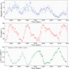 |
Figure 1. Top panel: Heliospheric magnetic field magnitude at 1 au as function of time, from OMNI data. Middle panel: heliospheric tilt angles, classical model results from the Wilcox Solar Observatory. Bottom panel: 1.28 GV GCR proton proxy intensities reported by Gieseler et al. (2017). |
The present study aims to study the influence of a stellar activity cycle on the transport of GCR protons and helium in the astrosphere of Proxima Centauri, an M5.5-dwarf located 1.3 pc from the Sun with a rocky exoplanet Prox Cen b4 located at 0.0485 au away from its star in the potential habitable zone with an orbital period of 11 days (Anglada-Escude et al. 2016). It should be noted that Proxima Centauri has been observed to be a strongly flaring star displaying many transient events (e.g. Shapley 1951; Fuhrmeister et al. 2011; Vida et al. 2019; Alvarado-Gomez et al. 2019), which leads to structures similar to the coronal mass ejections (Webb & Howard 2012; Moschou et al. 2019; Zic et al. 2020) and possibly global merged interaction regions such as those observed in the heliosphere during periods of higher solar activity (see, e.g., Burlaga & Ness 2000). This star is chosen as the transport of GCRs within its astrosphere has already been studied, albeit for approximately stellar minimum conditions, using a 3D GCR modulation model by Engelbrecht et al. (2024) and Light et al. (2025), and due to its relative proximity resulting in comparatively more observational information, particularly pertaining to cyclically-varying astrospheric parameters known to influence GCR transport, being available in the literature. As such, Proxima Centauri is a relatively slow-rotating star with a rotation period of 89.8 days (Klein et al. 2021); a surface magnetic field strength reported by Reiners & Basri (2008) using Zeeman broadening to be 600 G (see also the discussion by Garraffo et al. 2022), and by Klein et al. (2021) to be 200 G with a dipole component of 135 G using Zeeman-Doppler imaging (note that these different techniques sample magnetic fields on different scales); and a stellar cycle duration of approximately 7 years (Wargelin et al. 2017; Klein et al. 2021). Furthermore, close to maximum activity, a stellar tilt angle of 51° was reported by Klein et al. (2021). Beyond these observations, several studies have reported on the results of magnetohydrodynamic simulations for plasma parameters essential to the study of GCR modulation in Proxima Centauri’s astrosphere (see, e.g., Herbst et al. 2020b; Engelbrecht et al. 2024), increasingly using Zeeman-Doppler imaging maps as direct inputs (e.g. Garraffo et al. 2016; Alvarado-Gomez 2020; Kavanagh et al. 2021; Garraffo et al. 2022). These provide key inputs for modulation models. The present study will employ observational (where available) and simulation-based inputs for simple, cyclically-varying analytical models for large-scale plasma parameters such as the astrospheric magnetic field (AMF) magnitude and stellar tilt angle, as well as for small-scale turbulence parameters such as magnetic variances and correlation scales. Although no observations or simulations for these latter quantities exist, these are known to be extremely important in modelling the diffusion coefficients of GCRs (see Engelbrecht et al. 2022), and have been observed to vary cyclically in the heliosphere, assuming larger values during periods of solar maximum, and smaller during solar minimum (e.g. Zhao et al. 2018; Engelbrecht & Wolmarans 2020). These will be scaled following the assumed AMF cyclic behaviour, following the observed temporal behaviour of these quantities in the heliosphere (Burger et al. 2022). These temporal scalings will be used as inputs to the numerical modulation code employed by Light et al. (2025), which solves the fully 3D Parker (1965) GCR transport equation in a physics-first manner, employing diffusion coefficients derived from the quasilinear theory (QLT, Jokipii 1966) and the nonlinear guiding center theory (NLGC, Matthaeus et al. 2003). Although to date no observations exist for a magnetic polarity cycle for Proxima Centauri, this behaviour has been observed in other slow-rotating M-dwarf stars (e.g. Lehmann et al. 2024), and will be taken into account in this study, in order to investigate the possible influence of such a polarity cycle on the astrospheric transport of GCRs. It should, however, be noted that cyclic magnetic polarity reversals have been reported on for a variety of stars (see, e.g., Jeffers et al. 2014; Boro Saikia et al. 2016; Rosen et al. 2016; See et al. 2016; Boro Saikia et al. 2022; Bellotti et al. 2025; Alvarado-Gomez et al. 2025). Temporally-varying GCR proton differential intensity spectra so calculated at the location of Proxima Centauri b will then be compared with heliospheric observations at 1 au.
As discussed in previous studies (e.g., Herbst et al. 2019b, 2024), the planetary high-energy particle environment influences (exo)planetary atmospheres, eventually leading to changes in atmospheric chemistry and climate. This, in turn, may affect potential biosignature signals such as ozone and methane, particularly in the case of Earth-like (i.e., N2-O2 dominated Grenfell et al. 2012) atmospheres. Thus, in general, including cosmic ray studies is essential for understanding and interpreting observations from the James Webb Space Telescope (JWST, e.g., Gardner et al. 2006, 2023) as well as future transmission spectra from the Atmospheric Remote-sensing Exoplanet Large-survey (Ariel, e.g., Tinetti et al. 2022) or the Extremely Large Telescope (ELT, see Padovani & Cirasuolo 2023). Cosmic rays further can drive the formation of prebiotic molecules (see, e.g., Rimmer et al. 2014; Airapetian et al. 2016), the building blocks of life, and high-energy GCRs in particular might have indirectly influenced the helicity of DNA (Globus & Blandford 2020). However, an enhanced flux of these energetic particles within an exoplanetary atmosphere can lead to enhanced radiation exposure and, with that, can induce DNA damage (see, e.g., Kennedy 2014). Thus, the manifold effects of cosmic rays within (exo)planetary atmospheres cannot be neglected in the context of (exo)planetary habitability.
The next section is devoted to a brief description of the GCR modulation model used, as well as the temporal profiles assumed for the various plasma inputs. The following section then introduces the atmospheric interaction model, after which model results will be presented. The study closes with a section discussing said results, and future prospects.
2. Modulation model
The present study solves the 3D Parker GCR transport equation stochastically (see, e.g., Pei et al. 2010; Engelbrecht & Burger 2015b; Strauss & Effenberger 2017, for more detail on this numerical technique), given in terms of the omnidirectional GCR phase space density f, related to to the differential intensity by j T = p 2 f where p is the particle momentum (see, e.g., Moraal 2013), and given by
 (1)
(1)
The above equation models the influence of various processes on GCR intensities as these particles enter an astrosphere, which include adiabatic energy changes (last term on the right) and convection with a stellar wind travelling at speed V s w (middle term on the right). Diffusion and drift effects are contained in the diffusion tensor K in the first term on the right hand side, given in AMF-aligned coordinates by (Burger et al. 2008)
![Mathematical equation: $$ \begin{aligned} \mathbf K^{\prime } =\left[\begin{array}{ccc} \kappa _{\perp ,3}&\kappa _{A}&0\\ -\kappa _{A}&\kappa _{\perp ,2}&0\\ 0&0&\kappa _{\parallel }\end{array}\right] \end{aligned} $$](/articles/swsc/full_html/2026/01/swsc250100/swsc250100-eq2.gif) (2)
(2)
with the subscripts on the diffusion coefficients κ denoting whether they describe diffusion parallel or perpendicular to the local AMF, related to an appropriate mean free path (MFP) by κ = v λ/3, with v the particle speed (see Shalchi 2009). In the stochastic approach, the Parker transport equation is rewritten as a set of equivalent Itō type differential equations (Zhang 1999) which can be solved by tracing a large number (in this study 10 000) of pseudoparticles per energy considered in a time-backward manner from the location of the exoplanet (in this case, Proxima Centauri b at 0.0485 au) to the simulation boundary. This is assumed to be at the location of Proxima Centauri’s termination shock, which is in this study modelled to be the latitudinally and azimuthally-dependent radial distance yielded by the MHD simulations of Proxima Centauri’s astrosphere presented by Engelbrecht et al. (2024). This distance can vary considerably, and is illustrated as function of azimuth in the ecliptic plane in Figure 2, where it extends to larger radial distances in the tail of the astrosphere (at 180°) than in the nose (at 0°). Although considerable GCR modulation is observed in the heliosheath (Stone et al. 2013), the termination shock location is chosen as the modulation boundary here, as Engelbrecht et al. (2024) demonstrated that most GCR modulation in Proxima Centauri’s astrosphere appear to happen within the termination shock. At this non-spherical modulation boundary, the differential intensity spectrum at the initial position (subscript ‘o’) can be calculated from the unmodulated boundary spectrum jB, often referred to as the local interstellar spectrum (LIS), using (Strauss et al. 2011)
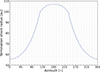 |
Figure 2. Radial distances at which Proxima Centauri’s termination shock is located in the ecliptic plane as function of azimuth, as yielded by the 3D MHD modelling presented by Engelbrecht et al. (2024), and employed in this study. Note that the astrospheric nose is located at 0°, and the tail at 180° azimuth. |
 (3)
(3)
where superscript e denotes an exit time or position. In this study, it is assumed that the LIS does not vary much over the relatively small (on galactic scales) distance between the Sun and Proxima Centauri, and accordingly employ the GCR proton expression proposed by Burger et al. (2008), given by
 (4)
(4)
which is a function of rigidity P, with P 0 = 1.0 GV, and is expressed here in units of particles m−2 s−1 sr−1 MeV−1. This expression is chosen for the purposes of comparison with the results of Engelbrecht et al. (2024), and it should be noted that Light et al. (2025) employ a boundary spectrum constructed by Moloto & Engelbrecht (2020) to fit Voyager observations at the heliospheric termination shock, in order to accommodate possible modulation effects in the astrosheaths of the various astrospheres those authors consider. For helium, a fit to the GALPROP5 simulations of GCR helium in the Galaxy by Boschini et al. (2020) as suggested by Engelbrecht et al. (2024) is used, given by
 (5)
(5)
in the same units as equation (4). For more detail as to the modulation code employed here, see Engelbrecht & Burger (2015b) and Light et al. (2025). Time-dependent differential intensities are calculated using an approach similar to that of Nagashima & Morishita (1980a); Nagashima & Morishita (1980b): astrospheric plasma parameters corresponding to a particular time are used as inputs to the model, which is then run sequentially for incremental timesteps. This approach has been shown to successfully capture the main temporal features of the solar cycle dependent modulation of GCRs in the heliosphere (see, e.g., Moloto & Engelbrecht 2020; Engelbrecht & Wolmarans 2020).
Diffusion coefficients derived assuming the composite slab+2D turbulence model (Matthaeus et al. 1990; Bieber et al. 1996) are used as inputs for Eq. (2). For the parallel MFP, the QLT expression derived by Teufel & Schlickeiser (2003) for a slab turbulence power spectrum with a wavenumber-independent energy-containing range and a Kolmogorov inertial range with spectral index s, is employed,
![Mathematical equation: $$ \begin{aligned} \lambda _{\parallel }(T) = \frac{3s}{\left(s - 1\right)}\frac{R(T)^2}{k_m(T)}\frac{B^2_0(T)}{\delta {B^2_{sl}(T)}}\left[\frac{1}{4{\pi }} + \frac{2R^{-s}(T)}{{\pi }(2 - s)(4 - s)}\right], \end{aligned} $$](/articles/swsc/full_html/2026/01/swsc250100/swsc250100-eq6.gif) (6)
(6)
where δ B s l 2 denotes the slab variance, k m the inverse of the slab correlation scale, and R = R L k m . This quantity is modelled to vary with time T in years after solar maximum as the various input parameters vary with this time. The perpendicular MFP use here is the NLGC result derived by Shalchi et al. (2004) for a 2D power spectrum with the same form as the slab spectrum assumed for λ ∥, with an inertial range spectral index given by 2ν = 5/3, and given by
![Mathematical equation: $$ \begin{aligned}&\lambda _{\perp }(T) =\nonumber \\&\left[{\alpha _d}^2{\sqrt{3{\pi }}}\frac{2\nu - 1}{\nu }\frac{\Gamma (\nu )}{\Gamma (\nu - 1/2)}{\lambda }_{2D}(T)\frac{{\delta }B^2_{2D}(T)}{B^2_0(T)}\right]^{2/3}{\lambda }_{\parallel }^{1/3}(T), \end{aligned} $$](/articles/swsc/full_html/2026/01/swsc250100/swsc250100-eq7.gif) (7)
(7)
where the subscript ‘2D’ denotes a 2D turbulence quantity, and it is assumed that  following the test-particle simulations of Matthaeus et al. (2003), although this quantity may be smaller in the heliosphere (see Els et al. 2024).
The off-diagonal coefficients κA in equation (2) describe drift effects due to a possible astrospheric current sheet, as well gradient and curvature drifts due to the geometry of the AMF. In the low-turbulence, weak scattering limit, these are given in terms of the maximal particle Larmor radius RL by (Forman et al. 1974)
 (8)
(8)
and can be related to the drift velocity by v d = ∇ × (κ A e B ) (e.g. Jokipii & Thomas 1981), where e B denotes a unit vector in the direction of the AMF. The drift velocity is then modelled following the approach of Burger (2012), assuming an angular extent of the astrospheric current sheet given by (Kota & Jokipii 2013)
![Mathematical equation: $$ \begin{aligned} \theta _{ns}(T) = \frac{\pi }{2} - \tan ^{-1} \left[ \tan \alpha (T) ~ \sin \left( \frac{\Omega r}{V_{sw}} \right) \right], \end{aligned} $$](/articles/swsc/full_html/2026/01/swsc250100/swsc250100-eq10.gif) (9)
(9)
where the stellar tilt angle α is now also a function of the time T in years after stellar maximum (see, e.g., Engelbrecht et al. 2019; Mohlolo et al. 2022, for further discussion on modelling drift effects numerically). The turbulent reduction of drift effects (see, e.g., Engelbrecht et al. 2017; van den Berg et al. 2021) are not considered here, as turbulence levels (as modelled here) are not expected to strongly influence particle drifts (see, e.g., the numerical simulations of Minnie et al. 2007; Els et al. 2024).
In order to model GCR transport coefficients self-consistently, temporal and spatial dependences for the large-scale plasma quantities they depend upon, as well as the small-scale turbulence quantities, need to be chosen. In terms of the spatial dependence of the astrospheric magnetic field, a Parker (1958) model is assumed, motivated by MHD simulation results (e.g. Herbst et al. 2022), given by
 (10)
(10)
which is normalised to a temporally-varying value of B 0(T) at 1 au, with parameter A = ±1 governing the sign of the magnetic field. The magnetic field lines of this AMF form spirals on cones of constant latitude, which are wound with an angle given by
 (11)
(11)
with Ω the stellar rotation rate, and V s w the stellar wind speed. As a first approach, a constant value of 1500 km s−1 is chosen for this latter quantity, motivated by the MHD simulations of Proxima Centauri’s astrosphere presented by Herbst et al. (2020b) within the termination shock. It should be noted that Kavanagh et al. (2021) report on a non spherically-symmetric stellar wind with a latitude-dependent speed that assumes a maximum value of 1200 km s−1, and such a stellar wind speed profile will be implemented in future studies, in a manner similar to that employed in heliospheric modulation studies (for an example, see Troskie et al. 2024). It is assumed that B 0(T) increases from a stellar minimum value of 2.4 nT (Engelbrecht et al. 2024) to 4.8 nT, making the assumption that the activity cycle reaches its peak when the magnetic cycle does, following Yadav et al. (2016). This doubling also reflects a factor of approximately 2 change in Proxima Centauri’s surface magnetic field inferred from X-ray observations over its cycle and convective dynamo simulations (see Wargelin et al. 2017; Alvarado-Gomez 2020; Garraffo et al. 2022), and is similar to the solar cycle-dependent behaviour of the heliospheric magnetic field (see Fig. 1). It should be noted however, that the Parker model may not fully capture the complexity of the astrospheric magnetic field. Indeed, it does not fully describe the complexities of the heliospheric magnetic field at solar maximum (Balogh & Smith 2001; Owens & Forsyth 2013), but is here implemented as a first modelling approach. The stellar tilt angle is assumed to vary from a stellar minimum value of 5°, as opposed to the assumption of 0° made in prior studies (implying a completely flat current sheet, see equation (9)) and motivated by heliospheric observations, to a maximum value of 51°, motivated by observations of Proxima Centauri (Klein et al. 2021). The magnetic polarity cycle length for Proxima Centauri is not yet known. As a first approach, it is here assumed that the AMF polarity will change at the time of full stellar maximum, as is the case for the Sun, which implies a magnetic polarity cycle twice the length of the stellar cycle. Such a long cycle choice is motivated by the slow rotation of Proxima Centauri: from observations of other stars, Bellotti et al. (2025) find that a faster magnetic polarity cycle is often associated with a greater rotation rate, albeit for a relatively small sample of stars.
Astrospheric turbulence quantities cannot yet be directly observed, and therefore are modelled here following the approach of Engelbrecht et al. (2024), where heliospheric models are scaled up (or down) by a factor related to the relative magnitude of the AMF to HMF magnitude at 1 au, which can then be varied as function of the stellar cycle through the accompanying variations in the astrospheric magnetic field. This choice is motivated by heliospheric observations of the solar cycle variations of these quantities, which increase or decrease with increases/decreases in the heliospheric magnetic field magnitude (Burger et al. 2022). Spatially, simple power-law radial dependences are chosen for magnetic variances and correlation scales. These are chosen so as to be in agreement with heliospheric observations (see, e.g., Zank et al. 1996; Smith et al. 2001; Pine et al. 2020; Burger & McKee 2023) as well as the results of turbulence transport modelling (see, e.g., Breech et al. 2008; Oughton et al. 2011; Adhikari et al. 2021; Oughton & Engelbrecht 2021). For the total magnetic variance,
 (12)
(12)
where a heliospheric value of 12.5 nT2 (Smith et al. 2006) at r 0 = 1 au is modified by the ratio of the astrospheric to the solar minimum heliospheric magnetic field magnitude, chosen here to be B H = 5 nT. As a first approach, the total variance is assumed to be composed of an 80% 2D component and a 20% slab component, after Bieber et al. (1994). The spatial dependence of the 2D correlation scale is also modelled following heliospheric observations (see Smith et al. 2001; Cuesta et al. 2022), assuming a value at 1 au that is scaled up from the heliospheric value reported by Weygand et al. (2011), such that
 (13)
(13)
with a temporal dependence again governed by that of the AMF. The slab correlation scale is modelled after the heliospheric ratio of these quantities reported on by Weygand et al. (2011), such that
 (14)
(14)
Given that detailed observations are not yet available, the temporal dependences of the quantities discussed above are modelled using a simple cosine dependence, given by
![Mathematical equation: $$ \begin{aligned} x=a+b\cos \left[\frac{2\pi T}{P_{c}}\right] \end{aligned} $$](/articles/swsc/full_html/2026/01/swsc250100/swsc250100-eq16.gif) (15)
(15)
with P c = 7 the stellar cycle length in years, and where a = (x max + x min)/2 and b = (x max − x min)/2, quantities that refer to the maximum and minimum values for the various plasma quantities modelled here, which are listed in Table 1. Note that the temporal profiles used here, as modelled with equation (15), do not take into account any transient structures due to flaring that may propagate outwards into the astrosphere, such as corotating interaction regions or merged interaction regions. As a first approach, however, these effects are omitted here, as it is at present unclear how such structures will evolve in Proxima Centauri’s astrosphere, which would require magnetohydrodynamic modelling (for a heliospheric example of such a study, see Wiengarten et al. 2015). The top two panels of Figure 3 illustrate the modelled stellar cycle dependences for the AMF magnitude at 1 au and the stellar tilt angle. Both drop from maximal values during stellar maximum (T = 0, 7 and 14 years) towards stellar minimum (T = 3.5 and 10.5 years), under the assumption that both will change in phase. As a first approach, the temporal profile employed here for the tilt angle α is not the same as that observed for the heliosphere, shown in Figure 1, which does not display a symmetric temporal profile in the years around to solar maximum (see, e.g., Smith 2001b). Should future observations motivate the use of such a profile, the analytical fit proposed by Burger et al. (2008) can potentially be modified and employed in subsequent studies. Magnetic variances and correlation scales (not shown) follow similar temporal profiles. The bottom panel of Figure 3 shows the parallel MFP (Eq. (6), red line), the perpendicular MFP (Eq. (7), blue line), and the drift scale (which is here, assuming the weak scattering limit, equal to the maximal Larmor radius RL found in equation (8), and shown as the green line in the figure) calculated at a rigidity of 1.28 GV as function of time after stellar maximum at 1 au. The parallel MFP assumes larger values during stellar maximum than during stellar minimum, and remains roughly two orders of magnitude larger than λ⊥ for all times shown, a factor similar to that expected in the heliosphere (see, e.g., Palmer 1982; Lang et al. 2024). The perpendicular MFP assumes larger values during stellar minima than during maxima, the opposite being true for the drift scale due to its dependence on the AMF magnitude, and remains larger than λ⊥, even during times of stellar maximum. This is surprising, as the drift scale drops below λ⊥ during solar maximum in the heliosphere, leading to GCR intensities relatively unaffected by drift effects during those periods (see, e.g., Engelbrecht & Moloto 2021).
Stellar minimum and maximum model inputs. See text for details.
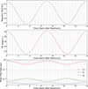 |
Figure 3. Top panel: Assumed temporal profile for Proxima Centauri’s AMF magnitude at 1 au, as function of years after full stellar maximum. Middle panel: Assumed temporal profile for Proxima Centauri’s tilt angle. Bottom panel: 1.28 GV GCR proton parallel and perpendicular MFPs (red and blue lines, respectively) as well as drift scales (green line), at 1 au. See text for details. |
3. Atmospheric interaction model
Stellar cycle-induced GCR intensity changes will directly influence the atmospheres of planets orbiting stars. To study the atmospheric effects of cosmic rays, Banjac et al. (2019) developed the Atmospheric Radiation Interaction Simulator (AtRIS), a GEANT4-based model allowing to compute induced secondary particle showers, ionisation rates, and radiation exposure in diverse exoplanetary atmospheres. AtRIS has successfully been validated and applied in solar system studies (e.g. Herbst et al. 2019a, 2020a; Guo et al. 2019; Winant et al. 2023) and beyond (e.g., Scheucher et al. 2020; Herbst et al. 2019b, 2024; Scherer et al. 2025; Light et al. 2025).
One of the main indicators of the atmospheric cosmic ray impact is the atmospheric ionisation which is directly linked to atmospheric chemistry and climate (e.g., Herbst et al. 2019b, 2024). Numerically speaking, the induced atmospheric ion pair production rate Q is described as
 (16)
(16)
Thereby, Y i (E, x) refers to the atmospheric ionisation yield given by 2π∫dθcos(θ)sin(θ)⋅(Δ E i /Δ x)/E ion, with E ion the average atmospheric ionisation energy6 and Δ E i /Δ x the mean specific energy loss of a primary particle of type i at a specific altitude x. The variable E c refers to the cutoff energy of the primary particle, the energy needed to reach specific locations at certain altitudes. In this study, E c is set at 10 MeV reflecting low magnetic shielding (i.e., polar regions at Earth).
AtRIS further provides a pre-calculated relative ionisation efficiency ℐ
R, j
(E
i
), the ratio between the average ionisation energy caused by a secondary particle of type j produced (e.g., p, n, e±, etc.) in a pre-selected phantom. We selected a human-mimicking phantom to study the effect on life as we know it from Earth. In particular, the International Commission on Radiation Units and Measurements (ICRU) phantom (McNair 1981) has been used. Of particular interest are the absorbed dose rates  given by
 (17)
(17)
Here, m ph denotes the phantom’s mass7. Convolving the results with the primary particle spectrum and summing over all energy bins and particle types gives the absorbed dose rate profiles.
4. Results
The top panel of Figure 4 shows differential intensities of GCR protons as function of kinetic energy computed at Proxima Centauri b during times of full stellar minimum (solid lines) and full stellar maximum (dashed lines) for both A > 0 (red lines) and A < 0 (blue lines) magnetic polarity conditions. Also shown are heliospheric observations of GCR protons at 1 au, taken during solar minimum periods of positive and negative magnetic polarity, reported by McDonald et al. (1992). As observed in the heliosphere, GCR intensities during stellar minimum are larger than during stellar maximum, indicating a clear influence of stellar cycle related changes in astrospheric plasma parameters on computed GCR intensities. Stellar minimum intensities are close to those reported on by Engelbrecht et al. (2024), but differ in that the difference in intensities for A < 0 and A > 0 is somewhat larger here. This is due to the fact that a tilt angle of 5° is assumed here, while Engelbrecht et al. (2024) assume a completely flat current sheet. This is reminiscent of the relationship between GCR intensity and tilt angle observed in the heliosphere, where intensities during A > 0 decrease sharply with small increases in α directly after solar minimum, while intensities remain relatively constant for similar changes during A < 0 (see, e.g., Lockwood & Webber 2005). It should be noted that stellar minimum intensities reported on here are larger than those reported on by Light et al. (2025), due to differences in the boundary spectra. The intensities for both stellar maximum and stellar minimum in Figure 4 also remain well above heliospheric observations. This is true even during stellar maximum, and is due to the slow rotation of the star, which leads to a highly underwound AMF. which in turn leads to diffusion parallel to the AMF contributing largely towards the inward transport of GCRs (Light et al. 2025). During stellar minimum, A < 0 intensities remain above A > 0 intensities, as reported on by Engelbrecht et al. (2024), and in contrast to what is observed in the heliosphere. This can again be related to the slow stellar rotation rate, in that drifts due to gradients in, and curvatures of, the AMF, which govern the inward transport of GCR protons during A > 0, are accordingly less effective than current sheet drift, which governs the inward transport of GCRs during A < 0. This picture is somewhat reversed during stellar maximum, where, in contrast with what is observed in the heliosphere during solar maximum, drift effects still appear to play a role, and where A > 0 intensities are now slightly larger than A < 0 intensities. This is not entirely unexpected, as from the bottom panel of Figure 3 it can be seen that the drift scale remains larger than the perpendicular diffusion coefficient even over stellar maximum periods, in contrast to the heliosphere. As the astrospheric current sheet as modelled by equation (9) would be considerably wavier due to the larger tilt angle, particles have further to drift along this structure, leading to lower intensities. It should be noted that the stellar maximum spectra shown here differ from those computed by Light et al. (2025) where a tilt of 51° was assumed, with all other parameters held to stellar minimum values. From their results, it could be concluded that stellar cyclic effects would be negligible during A < 0, and considerably smaller than can be seen in Figure 4 for A > 0. These differences arise because that study did not include the effects of a larger AMF magnitude during stellar maximum and did not vary magnetic variances and correlation scale with stellar cycle either, as is done here, thereby not fully modelling the influence of stellar cycle variations on GCR transport coefficients, and highlighting the need to do so. GCR Helium intensities computed at Proxima Centauri b are shown in the middle panel of Figure 4. These behave very similarly to the GCR protons, with intensities during stellar minimum and maximum remaining well above observed heliospheric intensities at 1 au reported by Adriani et al. (2013). Charge-sign dependent modulation can also still be discerned during full stellar maximum.
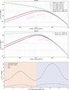 |
Figure 4. Top panel: GCR proton differential intensities as function of kinetic energy, calculated at 0.0485 au for A > 0 (red lines) and A < 0 (blue lines) magnetic polarity conditions. Solid lines indicate intensities calculated during full stellar minimum, dashed during full stellar maximum. Also shown are the Burger et al. (2008) LIS (green line), and heliospheric observations at Earth reported by McDonald et al. (1992). Middle panels: Same as top panel, but for GCR Helium. Green dashed line denotes the Boschini et al. (2020) LIS employed here, while stars indicate A < 0 PAMELA observations reported by Adriani et al. (2013). Bottom panel: 1.28 and 0.44 GV GCR proton intensities (green and black lines, respectively) calculated at 0.05 au as function of time after full stellar maximum. |
The bottom panel of Figure 4 shows 1.28 GV (0.65 GeV, green line) and 0.44 GV (0.1 GeV, black line) GCR intensities computed as function of years after full stellar maximum at Proxima Centauri b. Given the similarity in relative behaviour between stellar minimum and maximum intensities for GCR protons and helium discussed above, only proton intensities are shown here. Red and blue shadings indicate positive and negative magnetic polarity conditions, respectively, over a time period of twice the stellar cycle length. Note that the discrete jumps/drops in intensities just past the 7-year period is indicative of a change in magnetic polarity. This, similar to Kota & Jokipii (2013) is done discretely in the model, and not propagated outwards with time. Continuously propagating such a polarity change outward into the astrosphere will lead to a more continuous transition, as has been demonstrated in heliospheric models by, e.g., Moloto & Engelbrecht (2020), but is beyond the scope of the present study. The GCR modulation model is run consecutively for incrementally increased times, so that each run, and resulting intensity, is separated by three months, as indicated by the dots on the lines. The resulting intensity profiles are remarkably different to that seen for 1.28 GV GCR protons at 1 au in the heliosphere (bottom panel of Fig. 1). For the 1.28 GV protons at Proxima Centauri b, only a small variation from minimum to maximum can be seen, and the stellar minimum peak profiles during A > 0 are only moderately different from those computed for A < 0 conditions. As can be seen in the top panel of Figure 4, the amplitude of the variation in GCR intensity from a peak during stellar minimum to a trough during stellar maximum varies as function of energy, being more marked for the 0.44 GV protons (where more modulation occurs), as well as being larger during A < 0 than during A > 0. For the 1.28 GV protons, the ratio between full stellar minimum (at 3.5 and 10.5 years here) and full maximum (at 0 and 14 years in the figure) intensities is 1.13 during A > 0, and 1.12 during A < 0, in contrast with the peak-to trough ratio of an approximately consistent value of 3 observed in the heliosphere at this rigidity, demonstrating a more modest dependence of GCR intensities on stellar cycle-varying plasma parameters, arising from the influence of the slow rotation of the parent star on GCR transport that leads to less modulation. At lower energies, however, the effect of taking into account the stellar cycle variation of parameters becomes much more significant: at 0.1 GeV n−1, the A > 0 ratio is 1.49, while during A < 0 it is 1.84. Differences in peaks during different magnetic polarity conditions are still not as striking as observed in the heliosphere: the A < 0 peak profile at 0.44 GV is only somewhat sharper than the very slightly plateaued A > 0 profile. Lastly, it should be noted that the smoothness of the GCR temporal profiles in the bottom panel of Figure 4 reflects the smoothness of the input temporal profiles of the plasma quantities employed in the model (Eq. (15)). Taking into account more complex, transient phenomena such as corotating interaction regions or global merged interaction regions, would greatly alter this behaviour. These have been shown to lead to decreases in GCR intensities in the heliosphere, as they act as transient barriers to the inward diffusion of GCRs (see, e.g., Burlaga 1984; Potgieter et al. 1993; le Roux & Fichtner 1999; Richardson et al. 2022; Burlaga et al. 2003) due to enhanced turbulence (see, e.g., Wiengarten et al. 2015; Strauss et al. 2016), particularly towards solar maximum. As such, the GCR intensities shown in Figure 4 can possibly be interpreted as representing an upper estimate.
Based on the GCR spectra discussed in Section 2, Figure 5 shows the atmospheric GCR-induced ion-pair production rate (left panel) and absorbed dose rate (middle panel) profiles modelled with AtRIS. Here, the contributions due to the primary proton (dashed lines) and helium (dotted lines) GCRs are separated and the total values (solid lines) used in what follows are displayed. The right panel further shows the helium particle contribution to the total ion pair production rates (blue line) as well as the absorbed dose rates (orange line). The results account for the A < 0 stellar minimum conditions. As can be seen, the helium contribution to the ionisation rates at altitudes above 23 km and absorbed dose rates above 11 km exceeds 20%, highlighting the necessity of including helium spectra, particularly when ionisation rates – crucial inputs to atmospheric chemistry and climate models – are derived.
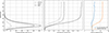 |
Figure 5. GCR-induced atmospheric ion-pair production rates (left panel) and absorbed dose rates (middle panel) due to primary protons (dashed lines) and helium (dotted lines); solid lines represent the sum of both. The right panel shows the helium contribution. |
In addition, Figure 6 shows the stellar cycle induced changes in atmospheric ionisation (left panels) and absorbed dose rates (right panels), calculated using both the primary proton and helium GCR contributions. The upper panels display the full stellar maximum condition induced changes in years 0, 7, and 14 corresponding to stellar maximum while the lower panels refer to the full stellar minimum conditions during A > 0 conditions (i.e., at year 3.5 after maximum) and during A < 0 conditions (i.e., at year 10.5 after maximum). In all cases, the petrol bands represent the induced changes over the entire time frame after full stellar maximum. The maximum induced changes over the entire time frame (i.e., years 0 and 10.5) are up to 28% in atmospheric ionisation rates and up to 5% in absorbed dose rate values. The changes of the full stellar maximum conditions in years 0 and 7 are almost identical while showing an increase of up to 8% and 2%, respectively. The A < 0 conditions induce changes in the order of up to 12% (2%) in atmospheric ionisation (absorbed dose rates) higher than the A > 0 conditions.
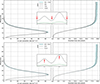 |
Figure 6. GCR induced ion pair production rates (left panels) and absorbed dose rates (right panels), during the full stellar maximum conditions in years 0, 7, and 14 (the first two give identical values) in the upper panels and the full stellar minimum conditions in years 3.5 (A > 0) and 10.5 (A < 0) in the lower panels. The petrol-shaded envelope shows the entirety of the variations within these 14 years. |
5. Conclusions
Stellar cycle-related changes in the astrospheric magnetic field magnitude and stellar tilt angle have been demonstrated here, for the first time, using a 3D ab initio cosmic ray modulation model, to lead to stellar cycle-related changes in GCR proton and Helium intensities at the location of Proxima Centauri b. Qualitatively, these intensity variations follow the same pattern as those observed in the heliosphere: peak intensities occur during stellar minima, and minimum intensities during periods of high stellar activity. Quantitatively, the stellar cycle variations of GCR intensities in Proxima Centauri’s astrosphere are much more modest than those observed at Earth. During stellar minima the intensities computed for negative magnetic polarity conditions are larger than those computed for positive polarity conditions, again in contrast with what is usually observed during solar minima, and drift effects persist even during stellar maxima, which again contrasts with the essentially drift free GCR propagation observed in the heliosphere during solar maximum. Intriguingly, even though GCR proton and Helium temporal intensity profiles display minima during stellar maximum periods, these intensities remain significantly above solar minimum observations at Earth. This is due to a combination of factors, as reported by Engelbrecht et al. (2024) and Light et al. (2025). The slow rotation of Proxima Centauri leads to an underwound astrospheric magnetic field, which allows for enhanced particle diffusion into the astrosphere along astrospheric magnetic field lines, which is coupled with the effects of a smaller magnetic field magnitude, leading to larger particle Larmor radii and hence more efficient drift effects. The significance of the interplay of such inherently 3D phenomena highlights the need for 3D modelling of energetic particle transport in stellar astrospheres. Furthermore, the idiosyncrasies of stellar cycle-related effects on the temporal variation of GCR intensities in the astrosphere highlight the differences in these effects from what would be expected of them based on heliospheric observations. We further investigated the impact of GCR modulation-induced stellar cyclicity effects on an assumed Earth-like atmosphere for Prox Cen b as employed by Engelbrecht et al. (2024). Similar to the solar system, stronger modulation results in lower GCR-induced atmospheric ionisation and radiation exposure. However, changes exceeding 20% moderately affect the atmosphere due to variations in GCR flux at altitudes above 20 km. As exoplanetary atmospheric transmission spectra rely on data regarding atmospheric chemistry in the upper layers, this highlights the necessity for more precise information on GCR-induced background ionisation and radiation exposure in order to effectively interpret future observations from JWST, Ariel and the ELT for transiting exoplanets orbiting stars that display stellar cyclic behaviour.
As more observations of cyclic behaviour become available for a greater number of (potentially) exoplanet-hosting stars, these effects will need to be taken into account in particle transport modelling endeavours, so as to ascertain their significance in influencing the ionizing radiation environments of their (potential) exoplanets. The present study provides a first theoretical and modelling framework to do so in as self-consistent a manner as possible. However, future GCR modulation studies will also need to take into account the influence of transient, large-scale structures, such as corotating interaction regions, that can arise as a result of stellar flaring. The current model also employs parametric scalings for the spatial dependences of basic turbulence quantities used to compute GCR diffusion coefficients. This is a limitation, in that these are motivated by heliospheric observations. Future studies will include turbulence transport modelling, such as already has been done for the heliosphere (see, e.g. Oughton & Engelbrecht 2021; Adhikari et al. 2021) and for a young-Sun proxy star (Engelbrecht et al. 2026), to provide more theoretically self-consistent turbulence inputs for our GCR modulation code that are appropriate to Proxima Centauri’s astrosphere, so as to provide as realistic as possible estimations of the radiation environments of exoplanets orbiting active stars.
Acknowledgments
We acknowledge use of NASA/GSFC’s Space Physics Data Facility’s OMNIWeb service, and OMNI data. The editor thanks two anonymous reviewers for their assistance in evaluating this paper.
Funding
Part of this work was funded by the Research Council of Norway (RCN), through its Centre of Excellence funding scheme, project number 332523 (PHAB, Centre for Planetary Habitability).
Conflict of interest
The authors declare no Conflict of Interest.
Data availability statement
The data generated for this study are available on request from the corresponding author.
References
- Adhikari L, Zank GP, Zhao L. 2021. The transport and evolution of MHD turbulence throughout the heliosphere: Models and observations. Fluids 6(10): 368. https://doi.org/10.3390/fluids6100368, https://www.mdpi.com/2311-5521/6/10/368. [Google Scholar]
- Adriani O, Barbarino GC, Bazilevskaya GA, Bellotti R, Boezio M, et al. 2013. Measurement of the isotopic composition of Hydrogen and Helium nuclei in cosmic rays with the PAMELA experiment. Astrophys J 770(1): 2. https://doi.org/10.1088/0004-637X/770/1/2. [Google Scholar]
- Agarwal R, Mishra RK. 2008. Solar cycle phenomena in cosmic ray intensity up to the recent solar cycle. Phys Lett B 664(1–2): 31–34. https://doi.org/10.1016/j.physletb.2008.04.057. [Google Scholar]
- Ahluwalia HS. 2000. On galactic cosmic ray flux decrease near solar minima and IMF intensity. Geophys Res Lett 27(11): 1603–1606. https://doi.org/10.1029/2000GL003759, https://agupubs.onlinelibrary.wiley.com/doi/abs/10.1029/2000GL003759. [Google Scholar]
- Airapetian VS, Glocer A, Gronoff G, Hébrard E, Danchi W. 2016. Prebiotic chemistry and atmospheric warming of early Earth by an active young Sun. Nat Geosci 9(6): 452–455. httpss://doi.org/10.1038/ngeo2719. [Google Scholar]
- Alvarado-Gómez JD, Drake JJ, Garraffo C, Cohen O, Poppenhaeger K, et al. 2020. An Earth-like stellar wind environment for Proxima Centauri c. Astrophys J 902(1): L9. https://doi.org/10.3847/2041-8213/abb885. [Google Scholar]
- Alvarado-Gómez JD, Drake JJ, Moschou SP, Garraffo C, Cohen O, et al. 2019. Coronal response to magnetically suppressed CME events in M-dwarf stars. Astrophys J 884(1): L13. https://doi.org/10.3847/2041-8213/ab44d0. [Google Scholar]
- Alvarado-Gómez JD, Hussain GAJ, Amazo-Gómez EM, Xu Y, Poppenhäger K, et al. 2025. Far beyond the Sun: III. The magnetic cycle of ı Horologii. Astron Astrophys 704: A68. https://doi.org/10.1051/0004-6361/202555349. [Google Scholar]
- Anglada-Escudé G, Amado PJ, Barnes J, Berdiñas ZM, Butler RP, et al. 2016. A terrestrial planet candidate in a temperate orbit around Proxima Centauri. Nature 536(7617): 437–440. https://doi.org/10.1038/nature19106. [CrossRef] [Google Scholar]
- Balogh A, Smith EJ. 2001. The heliospheric magnetic field at solar maximum: Ulysses observations. Space Sci Rev 97: 147–160. https://doi.org/10.1023/A:1011854901760. [Google Scholar]
- Banjac S, Herbst K, Heber B. 2019. The Atmospheric Radiation Interaction Simulator (AtRIS): Description and validation. J Geophys Res: Space Phys 124(1): 50–67. https://doi.org/10.1029/2018JA026042, https://agupubs.onlinelibrary.wiley.com/doi/abs/10.1029/2018JA026042. [Google Scholar]
- Bellotti S, Petit P, Jeffers SV, Marsden SC, Morin J, et al. 2025. A BCool survey of stellar magnetic cycles. Astron Astrophys 693: A269. https://doi.org/10.1051/0004-6361/202452378. [Google Scholar]
- Bieber JW, Matthaeus WH, Smith CW, Wanner W, Kallenrode M-B, et al. 1994. Proton and electron mean free paths: The Palmer consensus revisited. Astrophys J 420: 294. https://doi.org/10.1086/173559. [CrossRef] [Google Scholar]
- Bieber JW, Wanner W, Matthaeus WH. 1996. Dominant two-dimensional solar wind turbulence with implications for cosmic ray transport. J Geophys Res 101(A2): 2511–2522. https://doi.org/10.1029/95JA02588. [Google Scholar]
- Boro Saikia S, Jeffers SV, Morin J, Petit P, Folsom CP, et al. 2016. A solar-like magnetic cycle on the mature K-dwarf 61 Cygni A (HD 201091). Astron Astrophys 594: A29. https://doi.org/10.1051/0004-6361/201628262. [Google Scholar]
- Boro Saikia S, Lüftinger T, Folsom CP, Antonova A, Alecian E, et al. 2022. Time evolution of magnetic activity cycles in young suns: The curious case of κ Ceti. Astron Astrophys 658: A16. https://doi.org/10.1051/0004-6361/202141525. [Google Scholar]
- Boschini MJ, Della Torre S, Gervasi M, Grandi D, Jóhannesson G, et al. 2020. Inference of the local interstellar spectra of cosmic-ray nuclei Z ≤ 28 with the GALPROP-HELMOD framework. Astrophys J Supp 250(2): 27. https://doi.org/10.3847/1538-4365/aba901. [Google Scholar]
- Breech B, Matthaeus WH, Minnie J, Bieber JW, Oughton S, et al. 2008. Turbulence transport throughout the heliosphere. J Geophys Res Space Phys 113(A8): A08105. https://doi.org/10.1029/2007JA012711. [Google Scholar]
- Burger RA. 2012. Modeling drift along the heliospheric wavy neutral sheet. Astrophys J 760(1): 60. https://doi.org/10.1088/0004-637X/760/1/60. [Google Scholar]
- Burger RA, Krüger TPJ, Hitge M, Engelbrecht NE. 2008. A fisk-parker hybrid heliospheric magnetic field with a solar-cycle dependence. Astrophys J 674(1): 511–519. https://doi.org/10.1086/525039. [Google Scholar]
- Burger RA, McKee SR. 2023. Evaluation and analysis of Voyager 1 48-s resolution magnetic field data. Adv Space Res 71(11): 4916–4922. https://doi.org/10.1016/j.asr.2023.01.033. [Google Scholar]
- Burger RA, Nel AE, Engelbrecht NE. 2022. Spectral properties of the N component of the heliospheric magnetic field from IMP and ACE observations for 1973–2020. Astrophys J 926(2): 128. https://doi.org/10.3847/1538-4357/ac4741. [Google Scholar]
- Burlaga LF. 1984. MHD processes in the outer heliosphere. Space Sci Rev 39: 255–316. [Google Scholar]
- Burlaga LF, Ness NF. 2000. Merged interaction regions observed by Voyagers 1 and 2 during 1998. J Geophys Res 105(A3): 5141–5148. https://doi.org/10.1029/1999JA000379. [Google Scholar]
- Burlaga LF, Wang C, Richardson JD, Ness NF. 2003. Large-scale magnetic field fluctuations and development of the 1999–2000 global merged interaction region: 1–60 AU. Astrophys J 585: 1158–1168. [Google Scholar]
- Caballero-Lopez RA, Engelbrecht NE, Richardson JD. 2019. Correlation of long-term cosmic-ray modulation with solar activity parameters. Astrophys J: 883(1): 73. https://doi.org/10.3847/1538-4357/ab3c57. [Google Scholar]
- Chahal D, Kamath D, de Grijs R, Montet BT, Chen X. 2025. Photometric activity cycles in fast-rotating stars: Revisiting the reality of stellar activity cycle branches. MNRAS 540(1): 668–687. https://doi.org/10.1093/mnras/staf754. [Google Scholar]
- Cuesta ME, Parashar TN, Chhiber R, Matthaeus WH. 2022. Intermittency in the expanding solar wind: Observations from Parker Solar Probe (0.16 au), Helios 1 (0.3–1 au), and Voyager 1 (1–10 au). Astrophys J Supp, 259(1): 23. https://doi.org/10.3847/1538-4365/ac45fa. [Google Scholar]
- Els PL, Engelbrecht NE, Lang JT, Strauss RD. 2024. The diffusion tensor of protons at 1 au: Comparing simulation, observation, and theory. Astrophys J 975(1): 134. https://doi.org/10.3847/1538-4357/ad7c44. [Google Scholar]
- Engelbrecht NE, Burger RA. 2015a. A comparison of turbulence-reduced drift coefficients of importance for the modulation of galactic cosmic-ray protons in the supersonic solar wind. Adv Space Res 55(1): 390–400. https://doi.org/10.1016/j.asr.2014.09.019. [Google Scholar]
- Engelbrecht NE, Burger RA. 2015b. Sensitivity of cosmic-ray proton spectra to the low-wavenumber behavior of the 2D turbulence power spectrum. Astrophys J 814(2): 152. https://doi.org/10.1088/0004-637X/814/2/152. [Google Scholar]
- Engelbrecht NE, Di Felice V. 2020. Uncertainties implicit to the use of the force-field solutions to the Parker transport equation in analyses of observed cosmic ray antiproton intensities. Phys Rev D 102(10): 103007. https://doi.org/10.1103/PhysRevD.102.103007. [Google Scholar]
- Engelbrecht NE, Effenberger F, Florinski V, Potgieter M, Ruffolo D, et al. 2022. Theory of cosmic ray transport in the heliosphere. Space Sci Rev 218: 33. https://doi.org/10.1007/s11214-022-00896-1. [Google Scholar]
- Engelbrecht NE, Herbst K, Scherer K, Oughton S, Airapetian VS. 2026. Particle transport from first principles in the early heliosphere: κ1 Ceti as a case study for the young sun. Astrophys J 998(1): 45. https://doi.org/10.3847/1538-4357/ae313e. [Google Scholar]
- Engelbrecht NE, Herbst K, Strauss RDT, Scherer K, Light J, et al. 2024. On the comprehensive 3D modeling of the radiation environment of Proxima Centauri b: A new constraint on habitability? Astrophys J 964(1): 89. https://doi.org/10.3847/1538-4357/ad2ade. [Google Scholar]
- Engelbrecht NE, Mohlolo ST, Ferreira SES. 2019. An improved treatment of neutral sheet drift in the inner heliosphere. Astrophys J 884(2): L54. https://doi.org/10.3847/2041-8213/ab4ad6. [Google Scholar]
- Engelbrecht NE, Moloto KD. 2021. An Ab initio approach to antiproton modulation in the inner heliosphere. Astrophys J 908(2): 167. https://doi.org/10.3847/1538-4357/abd3a5. [Google Scholar]
- Engelbrecht NE, Strauss RD, le Roux JA, Burger RA. 2017. Toward a greater understanding of the reduction of drift coefficients in the presence of turbulence. Astrophys J, 841(2): 107. https://doi.org/10.3847/1538-4357/aa7058. [Google Scholar]
- Engelbrecht NE, Wolmarans CP. 2020. Towards a deeper understanding of historic cosmic ray modulation during solar cycle 20. Adv Space Res 66(11): 2722–2732. https://doi.org/10.1016/j.asr.2020.09.022. [Google Scholar]
- Forbush SE. 1958. Cosmic-ray intensity variations during two solar cycles. J Geophys Res 63(4): 651–669. https://doi.org/10.1029/JZ063i004p00651, https://agupubs.onlinelibrary.wiley.com/doi/abs/10.1029/JZ063i004p00651. [CrossRef] [Google Scholar]
- Forman MA, Jokipii JR, Owens AJ. 1974. Cosmic-ray streaming perpendicular to the mean magnetic field. Astrophys J 192: 535–540. https://doi.org/10.1086/153087. [Google Scholar]
- Fuhrmeister B, Lalitha S, Poppenhaeger K, Rudolf N, Liefke C, et al. 2011. Multi-wavelength observations of Proxima Centauri. Astron Astrophys 534: A133. https://doi.org/10.1051/0004-6361/201117447. [Google Scholar]
- Gardner JP, Mather JC, Abbott R, Abell JS, Abernathy M, et al. 2023. The James Webb Space Telescope Mission. PASP 135(1048): 068001. https://doi.org/10.1088/1538-3873/acd1b5. [CrossRef] [Google Scholar]
- Gardner JP, Mather JC, Clampin M, Doyon R, Greenhouse MA, et al. 2006. The James Webb Space Telescope. Space Sci Rev 123(4): 485–606. https://doi.org/10.1007/s11214-006-8315-7. [Google Scholar]
- Garraffo C, Alvarado-Gómez JD, Cohen O, Drake JJ. 2022. Revisiting the space weather environment of Proxima Centauri b. Astrophys J 941(1): L8. https://doi.org/10.3847/2041-8213/aca487. [Google Scholar]
- Garraffo C, Drake JJ, Cohen O. 2016. The space weather of Proxima Centauri b. Astrophys J 833(1): L4. https://doi.org/10.3847/2041-8205/833/1/L4. [Google Scholar]
- Gieseler J, Heber B, Herbst K. 2017. An empirical modification of the force field approach to describe the modulation of galactic cosmic rays close to Earth in a broad range of rigidities. J Geophys Res Space Phys 122(11): 10 964–10 979. https://doi.org/10.1002/2017JA024763. [Google Scholar]
- Globus N, Blandford RD. 2020. The chiral puzzle of life. Astrophys J 895(1): L11. https://doi.org/10.3847/2041-8213/ab8dc6. [Google Scholar]
- Grenfell JL, Grießmeier J-M, von Paris P, Patzer ABC, Lammer H, et al. 2012. Response of atmospheric biomarkers to NOx-induced photochemistry generated by stellar cosmic rays for Earth-like planets in the habitable zone of M Dwarf stars. Astrobiology 12(12): 1109–1122. https://doi.org/10.1089/ast.2011.0682. [NASA ADS] [CrossRef] [Google Scholar]
- Guo J, Banjac S, Röstel L, Terasa JC, Herbst K, et al. 2019. Implementation and validation of the GEANT4/AtRIS code to model the radiation environment at Mars. J Space Weather Space Clim 9: A2. https://doi.org/10.1051/swsc/2018051. [Google Scholar]
- Hathaway DH. 2015. The solar cycle. Liv Rev Sol Phys 12(1): 4. https://doi.org/10.1007/lrsp-2015-4. [Google Scholar]
- Hedgecock PC. 1975. Measurements of the interplanetary magnetic field in relation to the modulation of cosmic rays. Sol Phys 42(2): 497–527. https://doi.org/10.1007/BF00149929. [Google Scholar]
- Herbst K, Baalmann L, Bykov A, Engelbrecht N, Ferreira S, et al. 2022. Astrospheres of planet-hosting cool stars and beyond: When modeling meets observations. Space Sci Rev 218: 29. https://doi.org/10.1007/s11214-022-00894-3. [Google Scholar]
- Herbst K, Banjac S, Atri D, Nordheim TA. 2020a. Revisiting the cosmic-ray induced Venusian radiation dose in the context of habitability. Astron Astrophys 633: A15. https://doi.org/10.1051/0004-6361/201936968. [Google Scholar]
- Herbst K, Banjac S, Nordheim TA. 2019a. Revisiting the cosmic-ray induced Venusian ionization with the Atmospheric Radiation Interaction Simulator (AtRIS). Astron Astrophys 624: A124. https://doi.org/10.1051/0004-6361/201935152. [Google Scholar]
- Herbst K, Bartenschlager A, Grenfell JL, Iro N, Sinnhuber M, et al. 2024. Impact of cosmic rays on atmospheric ion chemistry and spectral transmission features of TRAPPIST-1e. Astrophys J 961(2): 164. https://doi.org/10.3847/1538-4357/ad0895. [Google Scholar]
- Herbst K, Grenfell JL, Sinnhuber M, Rauer H, Heber B, et al. 2019b. A new model suite to determine the influence of cosmic rays on (exo)planetary atmospheric biosignatures. Validation based on modern Earth. Astron Astrophys 631: A101. https://doi.org/10.1051/0004-6361/201935888. [Google Scholar]
- Herbst K, Scherer K, Ferreira SES, Baalmann LR, Engelbrecht NE, et al. 2020b. On the diversity of M-star astrospheres and the role of galactic cosmic rays within. Astrophys J 897(2): L27. https://doi.org/10.3847/2041-8213/ab9df3. [Google Scholar]
- Hessman FV, Dhillon VS, Winget DE, Schreiber MR, Horne K, et al. 2010. On the naming convention used for multiple star systems and extrasolar planets. arXiv e-prints [arXiv:1012.0707]. https://doi.org/10.48550/arXiv.1012.0707 [Google Scholar]
- Hoeksema JT. 1995. The large-scale structure of the heliospheric current sheet during the ULYSSES epoch. Space Sci Rev 72(1–2): 137–148. https://doi.org/10.1007/BF00768770. [Google Scholar]
- Ibañez Bustos RV, Buccino AP, Nardetto N, Mourard D, Flores M, et al. 2025. Characterisation of magnetic activity of M dwarfs: Possible impact on surface brightness. Astron Astrophys 696: A230. https://doi.org/10.1051/0004-6361/202450348. [Google Scholar]
- Irving ZA, Saar SH, Wargelin BJ, do Nascimento J-D. 2023. Stellar cycles in fully convective stars and a new interpretation of dynamo evolution. Astrophys J 949(2): 51. https://doi.org/10.3847/1538-4357/acc468. [Google Scholar]
- Isenberg PA, Jokipii JR. 1979. Gradient and curvature drifts in magnetic fields with arbitrary spatial variation. Astrophys J 234: 746–752. [Google Scholar]
- Jeffers SV, Cameron RH, Marsden SC, Boro Saikia S, Folsom CP. et al., 2022. The crucial role of surface magnetic fields for stellar dynamos: Eridani, 61 Cygni A, and the Sun. Astron Astrophys 661: A152. https://doi.org/10.1051/0004-6361/202142202. [Google Scholar]
- Jeffers SV, Kiefer R, Metcalfe TS. 2023. Stellar activity cycles. Space Sci Rev 219(7): 54. https://doi.org/10.1007/s11214-023-01000-x. [Google Scholar]
- Jeffers SV, Petit P, Marsden SC, Morin J, Donati J-F, et al. 2014. Eridani: An active K dwarf and a planet hosting star? The variability of its large-scale magnetic field topology. Astron Astrophys 569: A79. https://doi.org/10.1051/0004-6361/201423725. [Google Scholar]
- Jokipii JR. 1966. Cosmic-ray Propagation. I. Charged particles in a random magnetic field. Astrophys J 146: 480. https://doi.org/10.1086/148912. [CrossRef] [Google Scholar]
- Jokipii JR, Thomas B. 1981. Effects of drift on the transport of cosmic rays. 4 – Modulation by a wavy interplanetary current sheet. Astrophys J 243: 1115–1122. [Google Scholar]
- Kavanagh RD, Vidotto AA, Klein B, Jardine MM, Donati J-F, et al. 2021. Planet-induced radio emission from the coronae of M dwarfs: The case of Prox Cen and AU Mic. MNRAS 504(1): 1511–1518. https://doi.org/10.1093/mnras/stab929. [NASA ADS] [CrossRef] [Google Scholar]
- Kennedy AR. 2014. Biological effects of space radiation and development of effective countermeasures. Life Sci Space Res 1: 10–43. https://doi.org/10.1016/j.lssr.2014.02.004, https://www.sciencedirect.com/science/article/pii/S2214552414000108. [Google Scholar]
- Khabarova O, Malandraki O, Malova H, Kislov R, Greco A, et al. 2021. Current sheets, plasmoids and flux ropes in the heliosphere. Part I. 2-D or not 2-D? General and observational aspects. Space Sci Rev 217(3): 38. https://doi.org/10.1007/s11214-021-00814-x. [Google Scholar]
- Kharayat H, Prasad L, Mathpal R, Garia S, Bhatt B. 2016. Study of cosmic ray intensity in relation to the interplanetary magnetic field and geomagnetic storms for solar cycle 23. Sol Phys 291: 603–611. https://doi.org/10.1007/s11207-016-0852-y. [Google Scholar]
- King JH, Papitashvili NE. 2005. Solar wind spatial scales in and comparisons of hourly Wind and ACE plasma and magnetic field data. J Geophys Res Space Phys 110(A2): A02104. https://doi.org/10.1029/2004JA010649. [Google Scholar]
- Klein B, Donati J-F, Hébrard ÉM, Zaire B, Folsom CP, et al. 2021. The large-scale magnetic field of Proxima Centauri near activity maximum. MNRAS 500(2): 1844–1850. https://doi.org/10.1093/mnras/staa3396. [Google Scholar]
- Kóta J. 2013. Theory and modeling of galactic cosmic rays: Trends and prospects. Space Sci Rev 176(1–4) 391–403. https://doi.org/10.1007/s11214-012-9870-8. [Google Scholar]
- Kota J, Jokipii JR. 1983. Effects of drift on the transport of cosmic rays. 6–A Three-dimensional model including diffusion. Astrophys J 265: 573–581. [Google Scholar]
- Lang JT, Strauss RD, Engelbrecht NE, van den Berg JP, Dresing N, et al. 2024. A detailed survey of the parallel mean free path of solar energetic particle protons and electrons. Astrophys J 971(1): 105. https://doi.org/10.3847/1538-4357/ad55c3. [Google Scholar]
- le Roux J. 1999. Time-dependent cosmic-ray modulation and global merged interaction regions. Adv Space Res 23(3): 491–499. https://doi.org/10.1016/S0273-1177(99)00112-X, https://www.sciencedirect.com/science/article/pii/S027311779900112X. [Google Scholar]
- le Roux JA, Fichtner H. 1999. Global merged interaction regions, the heliospheric termination shock, and time-dependent cosmic ray modulation. J Geophys Res 104(A3): 4709–4730. https://doi.org/10.1029/1998JA900089. [Google Scholar]
- Lehmann LT, Donati JF, Fouqué P, Moutou C, Bellotti S, et al. 2024. SPIRou reveals unusually strong magnetic fields of slowly rotating M dwarfs. MNRAS 527(2): 4330–4352. https://doi.org/10.1093/mnras/stad3472. [Google Scholar]
- Light J, Engelbrecht NE, Herbst K, Scherer KD. 2025. On the 3D transport of galactic cosmic rays in a selection of exoplanet-hosting astrospheres: the influence of stellar rotation. MNRAS 537(2): 2097–2111. https://doi.org/10.1093/mnras/staf164. [Google Scholar]
- Lockwood JA, Webber WR. 2005. Intensities of galactic cosmic rays of 1.5 GV rigidity at Earth versus the heliospheric current sheet tilt. J Geophys Res: Space Phys 110(A4): A04102. https://doi.org/10.1029/2004JA010880, https://agupubs.onlinelibrary.wiley.com/doi/abs/10.1029/2004JA010880. [Google Scholar]
- Manuel R, Ferreira SES, Potgieter MS, Strauss RD, Engelbrecht NE. 2011. Time-dependent cosmic ray modulation. Adv Space Res 47(9): 1529–1537. https://doi.org/10.1016/j.asr.2010.12.007. [Google Scholar]
- Matthaeus WH, Goldstein ML, Roberts DA. 1990. Evidence for the presence of quasi-two-dimensional nearly incompressible fluctuations in the solar wind. J Geophys Res 95: 20 673–20 683. https://doi.org/10.1029/JA095iA12p20673. [Google Scholar]
- Matthaeus WH, Qin G, Bieber JW, Zank GP. 2003. Nonlinear collisionless perpendicular diffusion of charged particles. Astrophys J 590: L53–L56. [Google Scholar]
- Mavromichalaki H, Paouris E, Karalidi T. 2007. Cosmic-ray modulation: An empirical relation with solar and heliospheric parameters. Sol Phys 245: 369–390. https://doi.org/10.1007/s11207-007-9043-1. [Google Scholar]
- McDonald FB. 1998. Cosmic-ray modulation in the heliosphere A phenomenological study. Space Sci Rev 83: 33–50. [Google Scholar]
- McDonald FB, Moraal H, Reinecke JPL, Lal N, McGuire RE. 1992. The cosmic radiation in the heliosphere at successive solar minima. J Geophys Res 97(A2): 1557–1570. https://doi.org/10.1029/91JA02389. [Google Scholar]
- McNair A. 1981. ICRU report 33 – Radiation quantities and units pub: International commission on radiation units and measurements, Washington D.C. USA issued 15 April 1980, pp.25. J Labelled Compd Radiopharm 18(9): 1398–1398. https://doi.org/10.1002/jlcr.2580180918. [Google Scholar]
- Mesquita AL, Rodgers-Lee D, Vidotto AA. 2021. The Earth-like Galactic cosmic ray intensity in the habitable zone of the M dwarf GJ 436. MNRAS 505(2): 1817–1826. https://doi.org/10.1093/mnras/stab1483. [NASA ADS] [CrossRef] [Google Scholar]
- Mesquita AL, Rodgers-Lee D, Vidotto AA, Atri D, Wood BE. 2022. Galactic cosmic ray propagation through M dwarf planetary systems. MNRAS 509(2): 2091–2101. https://doi.org/10.1093/mnras/stab3131. [Google Scholar]
- Minnie J, Bieber JW, Matthaeus WH, Burger RA. 2007. Suppression of particle drifts by turbulence. Astrophys J 670(2): 1149–1158. https://doi.org/10.1086/522026. [Google Scholar]
- Mohlolo ST, Engelbrecht NE, Ferreira SES. 2022. A detailed comparison of techniques used to model drift in numerical cosmic ray modulation models. Adv Space Res 69(6): 2574–2588. https://doi.org/10.1016/j.asr.2021.12.035. [Google Scholar]
- Moloto KD, Engelbrecht NE. 2020. A fully time-dependent Ab initio cosmic-ray modulation model applied to historical cosmic-ray modulation. Astrophys J 894(2): 121. https://doi.org/10.3847/1538-4357/ab87a2. [Google Scholar]
- Moloto KD, Engelbrecht NE, Burger RA. 2018. A Simplified Ab initio cosmic-ray modulation model with simulated time dependence and predictive capability. Astrophys J 859(2): 107. https://doi.org/10.3847/1538-4357/aac174. [Google Scholar]
- Moloto KD, Eugene Engelbrecht N, Strauss RD, Diedericks C. 2023. The Southern African neutron monitor program: A regional network to study global cosmic ray modulation. Adv Space Res 72(3): 830–843. https://doi.org/10.1016/j.asr.2022.05.044. [Google Scholar]
- Moraal H. 1976. Observations of the eleven-year cosmic-ray modulation cycle. Space Sci Rev 19(6): 845–920. https://doi.org/10.1007/BF00173707. [Google Scholar]
- Moraal H. 2013. Cosmic-ray modulation equations. Space Sci Rev 176(1–4): 299–319. https://doi.org/10.1007/s11214-011-9819-3. [Google Scholar]
- Moschou S-P, Drake JJ, Cohen O, Alvarado-Gómez JD, Garraffo C, et al. 2019. The stellar CME-flare relation: What do historic observations reveal? Astrophys J 877(2): 105. https://doi.org/10.3847/1538-4357/ab1b37. [Google Scholar]
- Nagashima K, Morishita I. 1980a. Long term modulation of cosmic rays and inferable electromagnetic state in solar modulating region. Planet Space Sci 28(2): 177–194. https://doi.org/10.1016/0032-0633(80)90094-X. [Google Scholar]
- Nagashima K, Morishita L. 1980b. Twenty-two year modulation of cosmic rays associated with polarity reversal of polar magnetic field of the sun. Planet Space Sci 28(2): 195–205. https://doi.org/10.1016/0032-0633(80)90095-1. [CrossRef] [Google Scholar]
- Nigro G. 2022. An argument in favor of magnetic polarity reversals due to heat flux variations in fully convective stars and planets. Astrophys J 938(1): 22. https://doi.org/10.3847/1538-4357/ac8d57. [Google Scholar]
- Oughton S, Engelbrecht NE. 2021. Solar wind turbulence: Connections with energetic particles. New Astron 83: 101507. https://doi.org/10.1016/j.newast.2020.101507. [Google Scholar]
- Oughton S, Matthaeus WH, Smith CW, Breech B, Isenberg PA. 2011. Transport of solar wind fluctuations: A two-component model. J Geophys Res Space Phys 116(A8): A08105. https://doi.org/10.1029/2010JA016365. [Google Scholar]
- Owens MJ, Forsyth RJ. 2013. The heliospheric magnetic field. Liv Rev Sol Phys 10(1): 5. https://doi.org/10.12942/lrsp-2013-5. [Google Scholar]
- Padovani P, Cirasuolo M. 2023. The extremely large telescope. Contemp Phys 64(1): 47–64. https://doi.org/10.1080/00107514.2023.2266921. [Google Scholar]
- Palmer ID. 1982. Transport coefficients of low-energy cosmic rays in interplanetary space. Rev Geophys Space Phys 20: 335–351. https://doi.org/10.1029/RG020i002p00335. [CrossRef] [Google Scholar]
- Parker EN. 1958. Dynamics of the interplanetary gas and magnetic fields. Astrophys J 128: 664. https://doi.org/10.1086/146579. [CrossRef] [Google Scholar]
- Parker EN. 1965. The passage of energetic charged particles through interplanetary space. Planet Space Sci 13(1): 9–49. https://doi.org/10.1016/0032-0633(65)90131-5. [CrossRef] [Google Scholar]
- Pei C, Bieber JW, Burger RA, Clem J. 2010. A general time-dependent stochastic method for solving Parker’s transport equation in spherical coordinates. J Geophys Res Space Phys 115(A12): A12107. https://doi.org/10.1029/2010JA015721. [Google Scholar]
- Pine ZB, Smith CW, Hollick SJ, Argall MR, Vasquez BJ, et al. 2020. Solar wind turbulence from 1 to 45 au. II. Analysis of inertial-range fluctuations using voyager and ACE observations. Astrophys J 900(2): 92. https://doi.org/10.3847/1538-4357/abab0f. [Google Scholar]
- Potgieter MS, Le Roux JA, Burlaga LF, McDonald FB. 1993. The role of merged interaction regions and drifts in the heliospheric modulation of cosmic rays beyond 20 AU: A computer simulation. Astrophys J 403: 760–768. [Google Scholar]
- Quenby J. 1984. The theory of cosmic-ray modulation. Space Sci Rev 176: 201–267. [Google Scholar]
- Reinecke JPL, Potgieter MS. 1994. An explanation for the difference in cosmic ray modulation at low and neutron monitor energies during consecutive solar minimum periods. J Geophys Res: Space Phys 99(A8): 14 761–14 767. https://doi.org/10.1029/94JA00792, https://agupubs.onlinelibrary.wiley.com/doi/abs/10.1029/94JA00792. [Google Scholar]
- Reiners A, Basri G. 2008. The moderate magnetic field of the flare star Proxima Centauri. Astron Astrophys 489(3): L45–L48. https://doi.org/10.1051/0004-6361:200810491. [Google Scholar]
- Richardson JD, Paularena KI, Wang C, Burlaga LF. 2002. The life of a CME and the development of a MIR: From the Sun to 58 AU. J Geophys Res: Space Phys 107(A4): SSH 1–1–SSH 1–9. https://doi.org/10.1029/2001JA000175, https://agupubs.onlinelibrary.wiley.com/doi/abs/10.1029/2001JA000175. [Google Scholar]
- Rimmer PB, Helling C, Bilger C. 2014. The influence of galactic cosmic rays on ion-neutral hydrocarbon chemistry in the upper atmospheres of free-floating exoplanets. Int J Astrobiol 13(2): 173–181. https://doi.org/10.1017/S1473550413000487. [Google Scholar]
- Rodgers-Lee D, Rimmer PB, Vidotto AA, Louca AJ, Taylor AM, et al. 2023. The energetic particle environment of a GJ 436 b-like planet. MNRAS 521(4): 5880–5891. https://doi.org/10.1093/mnras/stad900. [NASA ADS] [CrossRef] [Google Scholar]
- Rodgers-Lee D, Taylor AM, Vidotto AA, Downes TP. 2021. Stellar versus Galactic: The intensity of cosmic rays at the evolving Earth and young exoplanets around Sun-like stars. MNRAS 504(1): 1519–1530. https://doi.org/10.1093/mnras/stab935. [CrossRef] [Google Scholar]
- Rosén L, Kochukhov O, Hackman T, Lehtinen J. 2016. Magnetic fields of young solar twins. Astron Astrophys 593: A35. https://doi.org/10.1051/0004-6361/201628443. [Google Scholar]
- Sadovski AM, Struminsky AB, Belov A. 2018. Cosmic rays near Proxima Centauri b. Astron Lett 44(5): 324–330. https://doi.org/10.1134/S1063773718040072. [Google Scholar]
- Scherer K, Herbst K, Engelbrecht NE, Ferreira SES, Kleimann J, et al. 2025. Modeling the astrosphere of LHS 1140: On the differences of 3D magnetohydrodynamic single- and multi-fluid simulations and the consequences for exoplanetary habitability. Astron Astrophys 694: A106. https://doi.org/10.1051/0004-6361/202450324. [Google Scholar]
- Scheucher M, Herbst K, Schmidt V, Grenfell JL, Schreier F, et al. 2020. Proxima Centauri b: A strong case for including cosmic-ray-induced chemistry in atmospheric biosignature studies. Astrophys J 893(1): 12. https://doi.org/10.3847/1538-4357/ab7b74. [Google Scholar]
- See V, Jardine M, Vidotto AA, Donati J-F, Boro Saikia S, et al. 2016. The connection between stellar activity cycles and magnetic field topology. MNRAS 462(4): 4442–4450. https://doi.org/10.1093/mnras/stw2010. [CrossRef] [Google Scholar]
- Shalchi A. 2009. Nonlinear cosmic ray diffusion theories, vol. 362 of Astrophysics and Space Science Library. Springer, Berlin. https://doi.org/10.1007/978-3-642-00309-7. [Google Scholar]
- Shalchi A, Bieber JW, Matthaeus WH. 2004. Analytic forms of the perpendicular diffusion coefficient in magnetostatic turbulence. Astrophys J 604(2): 675–686. https://doi.org/10.1086/382128. [Google Scholar]
- Shapley H. 1951. Proxima Centauri as a flare star. Proc Natl Acad Sci USA 37(1): 15–18. http://www.jstor.org/stable/88208. [Google Scholar]
- Shea M, Smart D. 1981. Preliminary search for cosmic radiation and solar-terrestrial parameters correlated with the reversal of the solar magnetic field. Adv Space Res 1(3): 147–150. https://doi.org/10.1016/0273-1177(81)90036-3, http://www.sciencedirect.com/science/article/pii/0273117781900363. [Google Scholar]
- Simon Wedlund C, Gronoff G, Lilensten J, Ménager H, Barthélemy M. 2011. Comprehensive cal culation of the energy per ion pair or W values for five major planetary upper atmospheres. Ann Geophys 29(1): 187–195. [Google Scholar]
- Smith CW, Isenberg PA, Matthaeus WH, Richardson JD. 2006. Turbulent heating of the solar wind by newborn interstellar pickup protons. Astrophys J 638(1): 508–517. https://doi.org/10.1086/498671. [Google Scholar]
- Smith CW, Matthaeus WH, Zank GP, Ness NF, Oughton S, et al. 2001. Heating of the low-latitude solar wind by dissipation of turbulent magnetic fluctuations. J Geophys Res 106(A5): 8253–8272. https://doi.org/10.1029/2000JA000366. [Google Scholar]
- Smith EJ. 2001a. The heliospheric current sheet. J Geophys Res 106(A8): 15 819–15 832. [Google Scholar]
- Smith EJ. 2001b. The heliospheric current sheet. J Geophys Res 106(A8): 15 819–15 832. https://doi.org/10.1029/2000JA000120. [Google Scholar]
- Stone EC, Cummings AC, McDonald FB, Heikkila BC, Lal N, et al. 2013. Voyager 1 observes low-energy galactic cosmic rays in a region depleted of heliospheric ions. Science 341(6142): 150–153. https://doi.org/10.1126/science.1236408. [NASA ADS] [CrossRef] [Google Scholar]
- Strauss RD, le Roux JA, Engelbrecht NE, Ruffolo D, Dunzlaff P. 2016. Non-axisymmetric perpendicular diffusion of charged particles and their transport across tangential magnetic discontinuities. Astrophys J 825(1) 43. https://doi.org/10.3847/0004-637X/825/1/43. [Google Scholar]
- Strauss RD, Potgieter MS, Büsching I, Kopp A. 2012. Modelling heliospheric current sheet drift in stochastic cosmic ray transport models. Astrophys Space Sci 339(2): 223–236. [CrossRef] [Google Scholar]
- Strauss RD, Potgieter MS, Kopp A, Büsching I. 2011. On the propagation times and energy losses of cosmic rays in the heliosphere. J Geophys Res Space Phys 116(A12): A12105. https://doi.org/10.1029/2011JA016831. [Google Scholar]
- Strauss RDT, Effenberger F. 2017. A Hitch-hiker’s guide to stochastic differential equations. Solution methods for energetic particle transport in space physics and astrophysics. Space Sci Rev 212(1–2): 151–192. https://doi.org/10.1007/s11214-017-0351-y. [CrossRef] [Google Scholar]
- Strong AW, Moskalenko IV. 1998. Propagation of cosmic-ray nucleons in the galaxy. Astrophys J 509(1): 212–228. https://doi.org/10.1086/306470. [Google Scholar]
- Suárez Mascareño A, Rebolo R, González Hernández JI. 2016a. Magnetic cycles and rotation periods of late-type stars from photometric time series. Astron Astrophys 595: A12. https://doi.org/10.1051/0004-6361/201628586. [Google Scholar]
- Suárez Mascareño A, Rebolo R, González Hernández JI. 2016b. Magnetic cycles and rotation periods of late-type stars from photometric time series. Astron Astrophys 595: A12. https://doi.org/10.1051/0004-6361/201628586. [Google Scholar]
- Teufel A, Schlickeiser R. 2003. Analytic calculation of the parallel mean free path of heliospheric cosmic rays. II. Dynamical magnetic slab turbulence and random sweeping slab turbulence with finite wave power at small wavenumbers. Astron Astrophys 397: 15–25. https://doi.org/10.1051/0004-6361:20021471. [Google Scholar]
- Tinetti G, Eccleston P, Lueftinger T, Salvignol J-C, Fahmy S, et al. 2022. Ariel: Enabling planetary science across light-years. In European Planetary Science Congress, EPSC 2022–1114. https://doi.org/10.5194/epsc2022-1114. [Google Scholar]
- Troskie JS, Engelbrecht NE, Steyn PJ. 2024. Cosmic-ray transport in the presence of a fisk-type heliospheric magnetic field: Investigating the influence of drift. Astrophys J 970(2): 144. https://doi.org/10.3847/1538-4357/ad517e. [Google Scholar]
- Usoskin IG. 2023. A history of solar activity over millennia. Liv Rev Sol Phys 20(1): 2. https://doi.org/10.1007/s41116-023-00036-z. [CrossRef] [Google Scholar]
- van den Berg JP, Engelbrecht NE, Wijsen N, Strauss RD. 2021. On the turbulent reduction of drifts for solar energetic particles. Astrophys J 922(2): 200. https://doi.org/10.3847/1538-4357/ac2736. [Google Scholar]
- Vida K, Oláh K, Kővári Z, van Driel-Gesztelyi L, Moór A, et al. 2019. Flaring activity of Proxima Centauri from TESS observations: Quasiperiodic oscillations during flare decay and inferences on the habitability of Proxima b. Astrophys J 884(2): 160. https://doi.org/10.3847/1538-4357/ab41f5. [Google Scholar]
- Wang B-B, Bi X-J, Fang K, Lin S-J, Yin P-F. 2019. Time-dependent solar modulation of cosmic rays from solar minimum to solar maximum. Phys Rev D 100(6): 063006. https://doi.org/10.1103/PhysRevD.100.063006. [Google Scholar]
- Wargelin BJ, Saar SH, Pojmański G, Drake JJ, Kashyap VL. 2017. Optical, UV, and X-ray evidence for a 7-yr stellar cycle in Proxima Centauri. MNRAS 464(3): 3281–3296. https://doi.org/10.1093/mnras/stw2570. [NASA ADS] [CrossRef] [Google Scholar]
- Webb DF, Howard TA. 2012. Coronal mass ejections: Observations. Liv Rev Sol Phys 9(1): 3. https://doi.org/10.12942/lrsp-2012-3. [Google Scholar]
- Weygand JM, Matthaeus WH, Dasso S, Kivelson MG. 2011. Correlation and Taylor scale variability in the interplanetary magnetic field fluctuations as a function of solar wind speed. J Geophys Res Space Phys 116(A8): A08102. https://doi.org/10.1029/2011JA016621. [Google Scholar]
- Wiengarten T, Fichtner H, Kleimann J, Kissmann R. 2015. Implementing turbulence transport in the CRONOS framework and application to the propagation of CMEs. Astrophys J 805(2): 155. https://doi.org/10.1088/0004-637X/805/2/155. [Google Scholar]
- Winant A, Pierrard V, Botek E, Herbst K. 2023. The atmospheric influence on cosmic-ray-induced ionization and absorbed dose rates. Universe 9(12): 502. https://doi.org/10.3390/universe9120502, https://www.mdpi.com/2218-1997/9/12/502. [Google Scholar]
- Yadav RK, Christensen UR, Wolk SJ, Poppenhaeger K. 2016. Magnetic cycles in a dynamo simulation of fully convective M-star Proxima Centauri. Astrophys J 833(2): L28. https://doi.org/10.3847/2041-8213/833/2/L28. [Google Scholar]
- Zank GP, Matthaeus WH, Smith CW. 1996. Evolution of turbulent magnetic fluctuation power with heliospheric distance. J Geophys Res 101(A8): 17 093–17 108. https://doi.org/10.1029/96JA01275. [Google Scholar]
- Zhang M. 1999. A Markov stochastic process theory of cosmic-ray modulation. Astrophys J 513(1), 409–420. https://doi.org/10.1086/306857. [Google Scholar]
- Zhao LL, Adhikari L, Zank GP, Hu Q, Feng XS. 2018. Influence of the solar cycle on turbulence properties and cosmic-ray diffusion. Astrophys J 856(2): 94. https://doi.org/10.3847/1538-4357/aab362. [Google Scholar]
- Zic A, Murphy T, Lynch C, Heald G, Lenc E, et al. 2020. A flare-type IV burst event from Proxima Centauri and implications for space weather. Astrophys J 905(1): 23. https://doi.org/10.3847/1538-4357/abca90. [Google Scholar]
During A > 0 the HMF in the northern hemisphere points away from the Sun and towards it in the southern hemisphere, the opposite being true during A < 0.
By convention (see Hessman et al. 2010), exoplanets are named by adding a lowercase letter, starting at ’b’ and proceeding alphabetically in order of discovery, to the name of their host star.
At https://galprop.stanford.edu/, see also Strong & Moskalenko (1998).
For the N2-O2 dominated atmosphere assumed in this study, an average atmospheric ionisation energy of 32 eV is used (e.g., Simon Wedlund 2011).
With  (see, e.g., Herbst et al. 2020a).
Cite this article as: Engelbrecht NE and Herbst K. 2026. On stellar activity cycle-related cosmic ray modulation effects in the astrosphere of Proxima Centauri. J. Space Weather Space Clim. 16, 13. https://doi.org/10.1051/swsc/2026012.
All Tables
All Figures
|
Figure 1. Top panel: Heliospheric magnetic field magnitude at 1 au as function of time, from OMNI data. Middle panel: heliospheric tilt angles, classical model results from the Wilcox Solar Observatory. Bottom panel: 1.28 GV GCR proton proxy intensities reported by Gieseler et al. (2017). |
| In the text | |
|
Figure 2. Radial distances at which Proxima Centauri’s termination shock is located in the ecliptic plane as function of azimuth, as yielded by the 3D MHD modelling presented by Engelbrecht et al. (2024), and employed in this study. Note that the astrospheric nose is located at 0°, and the tail at 180° azimuth. |
| In the text | |
|
Figure 3. Top panel: Assumed temporal profile for Proxima Centauri’s AMF magnitude at 1 au, as function of years after full stellar maximum. Middle panel: Assumed temporal profile for Proxima Centauri’s tilt angle. Bottom panel: 1.28 GV GCR proton parallel and perpendicular MFPs (red and blue lines, respectively) as well as drift scales (green line), at 1 au. See text for details. |
| In the text | |
|
Figure 4. Top panel: GCR proton differential intensities as function of kinetic energy, calculated at 0.0485 au for A > 0 (red lines) and A < 0 (blue lines) magnetic polarity conditions. Solid lines indicate intensities calculated during full stellar minimum, dashed during full stellar maximum. Also shown are the Burger et al. (2008) LIS (green line), and heliospheric observations at Earth reported by McDonald et al. (1992). Middle panels: Same as top panel, but for GCR Helium. Green dashed line denotes the Boschini et al. (2020) LIS employed here, while stars indicate A < 0 PAMELA observations reported by Adriani et al. (2013). Bottom panel: 1.28 and 0.44 GV GCR proton intensities (green and black lines, respectively) calculated at 0.05 au as function of time after full stellar maximum. |
| In the text | |
|
Figure 5. GCR-induced atmospheric ion-pair production rates (left panel) and absorbed dose rates (middle panel) due to primary protons (dashed lines) and helium (dotted lines); solid lines represent the sum of both. The right panel shows the helium contribution. |
| In the text | |
|
Figure 6. GCR induced ion pair production rates (left panels) and absorbed dose rates (right panels), during the full stellar maximum conditions in years 0, 7, and 14 (the first two give identical values) in the upper panels and the full stellar minimum conditions in years 3.5 (A > 0) and 10.5 (A < 0) in the lower panels. The petrol-shaded envelope shows the entirety of the variations within these 14 years. |
| In the text | |
Current usage metrics show cumulative count of Article Views (full-text article views including HTML views, PDF and ePub downloads, according to the available data) and Abstracts Views on Vision4Press platform.
Data correspond to usage on the plateform after 2015. The current usage metrics is available 48-96 hours after online publication and is updated daily on week days.
Initial download of the metrics may take a while.