| Issue |
J. Space Weather Space Clim.
Volume 12, 2022
Topical Issue - Ionospheric plasma irregularities and their impact on radio systems
|
|
|---|---|---|
| Article Number | 22 | |
| Number of page(s) | 29 | |
| DOI | https://doi.org/10.1051/swsc/2022016 | |
| Published online | 29 June 2022 | |
Scientific Review
Modeling of ionospheric scintillation
1
Deutsches Zentrum für Luft- und Raumfahrt, Institut für Solar-Terrestrische Physik, Kalkhorstweg 53, 17235 Neustrelitz, Germany
2
Informatique Electromagnétisme Electronique Analyse Numérique (IEEA), Courbevoie 92400, France
* Corresponding author: This email address is being protected from spambots. You need JavaScript enabled to view it.
Received:
23
December
2021
Accepted:
18
May
2022
Abstract
A signal, such as from a GNSS satellite or microwave sounding system, propagating in the randomly inhomogeneous ionosphere, experiences chaotic modulations of its amplitude and phase. This effect is known as scintillation. This article reviews basic theoretical concepts and simulation strategies for modeling the scintillation phenomenon. We focused our attention primarily on the methods connected with the random phase screen model. For a weak scattering regime on random ionospheric irregularities, a single-phase screen model enables us to obtain the analytic expression for phase and intensity scintillation indices, as well as the statistical quantities characterizing the strength of scintillation-related fades and distortions. In the case of multiple scattering, the simulation with multiple phase screens becomes a handy tool for obtaining these indices. For both scattering regimes, the statistical properties of the ionospheric random medium play an important role in scintillation modeling and are discussed with an emphasis on related geometric aspects. As an illustration, the phase screen simulation approaches used in the global climatological scintillation model GISM are briefly discussed.
Key words: Scintillation / Phase screens / Propagation in random medium / Modeling
© D. Vasylyev et al., Published by EDP Sciences 2022
 This is an Open Access article distributed under the terms of the Creative Commons Attribution License (https://creativecommons.org/licenses/by/4.0), which permits unrestricted use, distribution, and reproduction in any medium, provided the original work is properly cited.
1 Introduction
The scintillation phenomenon is familiar to everyone who has looked at the sky during cloudless nights. By looking for some period of time, one can observe the remarkable twinkling of stars. These random changes in the apparent star brightness or its position are due to the random distortion of light coming from a star caused by refractive index irregularities in a turbulent troposphere. The fluctuation in brightness or, in other words, in intensity is one example of the scintillation phenomenon. The pulsation of star images (star dancing) is another manifestation of this phenomenon known as angular scintillation.
If we were able to sense the electromagnetic radiation at radio wavelength, we would similarly perceive scintillation of distant radio sources of celestial origin and from artificial satellites. In this case, scintillation is caused by random scattering on irregularities of electron density of the electrons and protons in the Earth ionosphere, solar wind, or in the interstellar medium. As the electron density varies as a random function of location, the associated refractive index changes similarly. Hence, as a plane wavefront of the incoming signal passes through the region where the refractive index is low, the velocity of radio waves will be high, and the wavefront will advance farther. With a higher refractive index, the wavefront is delayed. In combination, these effects will result in a corrugated wavefront and phase fluctuations. Some portions of the wavefront will be convex in the direction of propagation, and some of them will be concave. At some distance from the scattering region, the partial waves with such concave or convex wavefronts will interfere constructively or destructively, producing a complex intensity pattern.
This article will focus on ionospheric scintillation phenomena, i.e., amplitude or intensity and phase fluctuations. Amplitude scintillation is more intense in equatorial regions, while phase scintillation is more frequent and stronger at high latitudes (Aarons, 1982; Liu et al., 2012; Tsai et al., 2017). Amplitude scintillation normally occurs when the Fresnel dimension of the propagating radio signal is of the order of irregularity scales in the ionosphere. This condition is met for the post-sunset equatorial irregularities formed in equatorial F-spread and the equatorial plasma bubbles (Moorthy et al., 1979; Patel et al., 2009; Yokoyama & Stolle, 2017). The phase scintillation is primarily caused by steep ionospheric density gradients and irregularities formed in the cusp and auroral precipitation regions and polar cap patches (Spogli et al., 2009; Jiao & Morton, 2015). Fluctuations in phase in these regions are additionally enhanced due to geometric effects, i.e., the relative position of field-aligned irregularities and the signal path (Forte & Radicella, 2004). The occurrence of ionospheric scintillation is also strongly time-dependent. It varies daily, seasonal, and yearly and is more frequent during post-sunset hours at low latitudes (Basu et al., 1996; Huang et al., 2014a; Jin et al., 2018). During vernal and autumn equinoxes, there is a higher probability of scintillation (Muella et al., 2013; Jiao & Morton, 2015). Finally, the strength and occurrence of phase and intensity scintillation correlate with solar and geomagnetic activity at high latitudes (Abdu et al., 1998; Souto Fortes et al., 2015; Guo et al., 2017; Béniguel, 2019).
Intense phase and intensity fluctuations may have a strong negative impact on modern technical infrastructure, the robustness of some life-critical services, and the quality of scientific data acquired in remote-sensing measurement campaigns. Intensity scintillation causes the signals from a satellite to fade below the average level. If the level of fading exceeds some prescribed margin of a receiver, the signal becomes masked by the noise and cannot be reliably retrieved. Phase scintillation induces a frequency shift that is responsible for cycle slips in GNSS signals (Knight & Finn, 1998; Horvath & Crozier, 2007). When this shift exceeds the bandwidth of the phase lock loop, the satellite tracking might fail, and in some cases, the loss of lock with the satellite might follow (Conker et al., 2003; Aquino et al., 2005; Sreeja et al., 2011). For positioning, navigation, and timing (PNT) applications, such as precise point positioning (PPP), this effect can impair the functionality of this service, putting vital systems at risk.
In astronomical and remote sensing applications, scintillation may degrade the contrast and resolution of images as well as incorporate artifacts and increase the noise level in retrieved data. In radio astronomy, ionospheric and interplanetary scintillations lead to image wander, degradation of image contrast, pulse broadening of pulsar signals, angular broadening of point sources, and thus degradation of the resolving power of radio telescopes (Strom et al., 2001). In applications such as GNSS reflectometry, intensity scintillation has the greatest impact on the degradation of retrieval performance in altimetric and scatterometric applications (Camps et al., 2016). As the algorithms for the sounding of Earth and planetary atmospheres are usually based on ill-posed inversion problems (Leitinger, 2001), the introduction of additional sources of noise due to scintillation may considerably influence the performance of retrieval methods. In occultation measurements, strong refractive scintillation impacts the measured values of bending angle and contributes to the residual ionospheric error (Hinson, 1986; Carrano et al., 2011; Ludwig-Barbosa et al., 2020). The remarkable effect of intensity and phase scintillation on synthetic aperture radar (SAR) missions is the “azimuth streaking” notable as a spatial modulation in the position of optimal azimuth registration (Gray et al., 2000; Carrano et al., 2012; Sato et al., 2021). Other effects of scintillation that influence the performance of SAR are defocusing (Belcher, 2008; van de Kamp et al., 2009), signal decorrelation (Ishimaru et al., 1999), degradation of coherence properties Béniguel & Hamel (2011), and random phase perturbations (Rogers et al., 2014).
However, it should be noted that scintillation has not only negative effects. The knowledge of the scintillation level makes it possible to localize irregularities of the electron density in the ionosphere (Sokolovskiy, 2000), deduce the climatological trends for their occurrence (Siefring et al., 2011), retrieve the properties of ionospheric, interplanetary, and interstellar medium (Rickett, 1977; Bhattacharyya et al., 1992; Shishov et al., 2010), or even infer the structure of the local magnetic fields in planetary ionospheres (Hinson & Tyler, 1982; Hinson, 1984). In combination with other instrumentation, scintillation monitoring becomes a powerful tool for investigating the formation and evolution of ionospheric structures such as spread-F and equatorial plasma bubbles (Kelley et al., 2002).
Due to the aforementioned impact of scintillation on various important services and on remote sensing data products, the theoretical modeling and computer simulation of these phenomena were attracting the attention of researchers for more than seventy years (for review, see e.g. Ratcliffe, 1956; Gurvich & Tatarskii, 1975; Fante, 1975a; Crane, 1977; Yeh & Liu, 1982; Kravtsov, 1992; Priyadarshi, 2015). The first theoretical ideas on how to model scintillation were closely related to the emergent statistical theory of turbulence (Kolmogorov, 1941) and the development of the theory of random functions and corresponding methods of spectral analysis (see e.g. Rice, 1944, 1945). The former theory gave an understanding of how one can describe complex random systems such as turbulence or randomly inhomogeneous media, while the theory of random functions provided the rigorous mathematical apparatus for dealing with signals modulated randomly in phase and amplitude. The major theoretical milestones in such developments were connected with the need for a description of optical light propagation in tropospheric turbulence or sound waves in a turbulent ocean (Tatarski, 2016). To such landmarks belong the introduction of the concept of locally homogeneous random media (Obukhov, 1949), the development of Rytov’s theory of smooth perturbations (Obukhov, 1953), the derivation of field moment equations (Shishov, 1968), and asymptotic methods for solving such equations (Gochelashvily & Shishov, 1975; Yakushkin, 1975; Fante, 1975b). These concepts allow one to establish a rigorous mathematical apparatus for dealing with wave propagation in a random medium and obtain formulas of scintillation indices for multiple cases important in practice.
In connection with the ionospheric propagation, the first theoretical attempts to explain scintillation were associated with the diffraction theory (Ratcliffe, 1956). The propagation of electromagnetic waves in a random ionosphere has been proposed to be modeled via a thin sheet of material that modulates the wave amplitude and phase. The transmitted wave is then represented as a set of uniform infinite plane waves traveling in different directions. The values of corresponding directional cosines are considered to be governed by the specific angular spectrum (Booker & Clemmow, 1950). At some distance from the modulating sheet of material, the interference of plane waves forms a specific diffraction pattern in intensity. If the modulation strength of the thin sheet is a random function of position, the phase shifts of plane waves emanating from it, as well as the formed diffraction pattern are random functions of the position (Booker et al., 1950). In these initial approaches, the randomness of scattering directions, i.e., of the directional cosines values, is the driver of random modulation for both phase and amplitude directly behind the screen. However, it was soon realized that for most cases of radio wave propagation in the ionosphere, the amplitude modulation factor could be neglected, and the spectrum of random phase modulation is sufficient to model scintillation (Hewish, 1951). This concept of the phase-modulated sheet, called simply the phase screen, has become an extremely handy tool for studying and modeling ionospheric phase and amplitude scintillation.
Among further advances and milestones in phase screen modeling of scintillation, one can distinguish the incorporation of spatial anisotropy of field-aligned ionospheric irregularities in phase screen generation (Briggs & Parkin, 1963; Singleton, 1970a), the introduction of multiple-phase screens for a description of extended random media (Fejer, 1953), and the replacement of Gaussian spectra for phase screen generation with more realistic ones with power-law dependence (Rufenach, 1972). Further, Uscinski (1985) has shown that there exists a close resemblance between the methods of moment equations for electromagnetic wave amplitudes and the theory of multiple-phase screens. The popularity of phase screen simulations of scintillation was also growing due to advances in numerical mathematics. After developing the fast Fourier transform (FFT) algorithm (Cooley & Tukey, 1965) and the split-step algorithm for solving wave equations with a variable refractive index (Hardin et al., 1973), the FFT-based phase screen generation became spread out as the numerical method for both intensity and phase scintillation simulations.
There are many models of ionospheric scintillation based on the aforementioned fundamental concepts, either on heuristic ideas or on phenomenology. Many of them are collected and discussed in some detail in the review of Priyadarshi (2015), which briefly discusses scintillation mechanisms and the morphology of high- and low-latitude scintillation. Among analytical models, one should mention those developed by Bramley (1967), Fremouw & Rino (1973), Rino (1979a,b), Aarons (1985), Franke & Liu (1985), Hinson (1986), Retterer (2010). The prominent numerical climatological models are WBMOD1 (Fremouw & Secan, 1984; Secan et al., 1995, 1997), GISM2 (Béniguel, 2002; Béniguel & Hamel, 2011; Béniguel, 2019), SIGMA3 (Deshpande et al., 2014, 2016; Deshpande & Zettergren, 2019), and some related models for GNSS applications such as the Cornel model (Humphreys et al., 2009), the UPC/OE/RDA model (Camps et al., 2017), and the multi-frequency GNSS scintillation model (Rino et al., 2018). The models incorporating in situ data are the equatorial and high-latitude models of Basu et al. (1976, 1981), the WBMGRID4 model (Groves et al., 1997), and the Wernik-Alfonsi-Materassi (WAM) model (Wernik et al., 2007), to name just a few. Table 1 summarizes the major development stages of scintillation modeling from a historical perspective. Many mentioned models are used for scientific purposes as well as in services for scintillation prediction, determination of time periods and geographic areas with strong scintillation, warning systems, etc.
Scintillation models listed in chronological order. The used abbreviations are: WS – weak scattering, SS – strong scattering, IM – isotropic medium, AM – anisotropic medium, SPO – scintillation probability of occurrence, HL – high latitudes, LL – low latitudes, A – analytical form of indices, P – phenomenological model, DDM – data-driven model, PS – single phase screen model, MPS – multiple phase screen model, NS – numerical simulation, EFM – equations for field moments method, SSTH – synthetic scintillation time history simulation.
The present article reviews the basic methods and theories used in the modeling of ionospheric scintillation. Instead of reviewing the ideas and results for particular scintillation models, we have the intention to provide the basic theoretical framework for describing and modeling electromagnetic field propagation in a random ionosphere that is applicable to the majority of the models listed in Table 1. The principal focus of this article is on the scintillation modeling with phase screens, namely the single- and multiple-phase screen approaches. Section 2 presents the theoretical methods for describing the propagation of electromagnetic waves in a disordered medium. Here we derive the wave equation for an electromagnetic field propagating in the random ionospheric media. The solution to this equation can be obtained by effectively superposing the wave propagation in a vacuum together with the random modulation of its phase. Particularly, the statistical properties of this phase modulation are deduced from the power spectral densities of electron density fluctuations. Several popular models of such spectra are summarized in Section 3. Section 4 outlines the influence of geometric parameters of the communication link and scintillation-causing irregularities on the strength of the scintillation. We discuss in some detail the assumptions of flat- and spherical geometries in the problem of scattering on random ionospheric inhomogeneities. Geometric parameters such as zenith and azimuth angles of the link, shape, and direction of anisotropic ionospheric irregularities and propagation factors are discussed. The analytic results for scintillation indices that include these effects are given in Section 5. In particular, the indices obtained in the flat-geometry approximation serve as a basis of the WBMOD scintillation model. The provided results in the spherical-geometry case can be useful for the consistent extension of the WBMOD applicability to the arbitrary slant communication links. The extension of these results to the case of multiple scattering is given in Section 6, where we discuss the FFT-based multiple phase screen (MPS) simulation algorithm. The Global Ionospheric Scintillation Model (GISM) is used to exemplify the scintillation simulation via the MPS. Finally, some conclusions have been drawn in Section 7.
2 Theoretical models of scintillation
When propagating in a random medium, an electromagnetic wave undergoes chaotic distortions of its phase and amplitude (or, alternatively, its power or intensity). In order to analyze, predict and effectively mitigate the degradation of the transmitted signal encoded in such a wave, the probability distribution functions (PDFs) for random phase and amplitude are needed. In general, the construction of such PDFs requires knowledge of all their moments or cumulants. In practice, it appears that moments up to the second-order are of importance and could alone serve as proxy parameters characterizing affects of random media on the propagating signal. This restriction of the interest to low-order moments is driven by two factors. Firstly, for a strongly irregular medium, one would expect that the PDF of interest approaches the Gaussian distribution as a consequence of the limiting theorems of probability theory (Papoulis & Pillai, 2002). In this case, knowledge of the first and second-order moments is sufficient to determine the total PDF. Secondly, the most important information is generally contained in low-order moments. For example, the mean-field provides information on the way that the incident wave is attenuated on passing through the medium. The second field moments are related to the visibility of fringes of two interfering signals, yielding information on the angular spread and power of the propagating signal. The second intensity moment (fourth field moment) is useful for the characterization of intensity fluctuations of the transmitted wave.
For this reason, the following statistical moments and their combinations are of primary interest in studying the effects of a randomly inhomogeneous ionosphere on the propagation of radio and microwave signals: (1)
(1) (2)where E is the field amplitude, I is the field intensity, S is the phase departure of the wave detected by the observer. The statistical averaging (ensemble- or time-averaging) here and in the following is denoted as 〈...〉. Conventionally, the one-minute time averages are used for the scintillation metrics defined by equations (1) and (2). The proxy quantities S4 and σS are called the amplitude (or intensity) and phase scintillation indices, correspondingly. As can be seen from the definition, both indices provide information on how strong fluctuating intensity and phase differ from their regular or mean values.
Restricting our attention to the analysis of the second-order statistical moments (1), (2) is one of the simplifications made while treating scintillation phenomena from the theoretical perspective. In the following sections, we will make a number of further simplifications. We will neglect the bending of signal rays in the ionosphere and consider the depolarization effects caused by the propagation in the ionosphere to be negligibly small. For simplicity, the spherical shape of the Earth is assumed, but the flat Earth approximation is discussed in the appropriate context. The ionospheric plasma would be considered to be collisionless, its random variations would be treated by statistical means that again rely on second-order statistical quantities such as autocorrelation functions. The simplified model for autocorrelation properties of electron density fluctuations would be utilized for incorporating the anisotropy effects in scintillation phenomena due to scattering on field-aligned irregularities. The bulk of hte random ionosphere would be treated effectively as a set of thin random phase screens, whose temporal variation would be incorporated into the spatial variation with the help of the so-called Taylor hypothesis. In view of all these assumptions and simplifications, the resulting theoretical methods are quite capable of gaining insights into the nature of scintillation phenomena and to be used in computer simulations of scintillation fading levels.
In this section, we outline the theoretical foundations of signal wave propagation in a random ionospheric medium and discuss some approximations and assumptions used. In particular, we derive the wave equation for a signal wave propagating in a randomly inhomogeneous medium, which is the central equation in the forthcoming analysis. The solution of this equation is essential for the calculation of the scintillation indices, as will be shown in the following sections.
2.1 Wave propagation in random medium
Let us consider a plane wave propagating in z direction. This wave impinges a random medium that extends over the range 0 ≤ z ≤ Δz, cf. Figure 1. In this section, we restrict our consideration to the normal incidence case that will be generalized to the oblique incidence case in Section 4. The electromagnetic field of this wave we write as (3)where r = (x y z)T is the three-dimensional spatial coordinate vector, ω is the angular frequency, k = ω/c is the free-space wave number, c is the speed of light. The quantities E0 and f(r) are the time-independent field amplitudes for waves propagating in a vacuum and in a random medium, respectively.
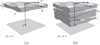 |
Figure 1 Geometry of propagation through a thin (a) and extended (b) random medium. These regimes correspond to a situation when the medium thickness is comparable to or larger than the typical scale |

If ε is the dielectric permittivity of the random medium, its general expression can be written as![Mathematical equation: $$ \epsilon (\mathbf{r},t)=\left\langle \epsilon (\mathbf{r},t)\right\rangle\left[1+{\delta \epsilon }(\mathbf{r},t)\right], $$](/articles/swsc/full_html/2022/01/swsc210095/swsc210095-eq4.gif) (4)where 〈ε〉 is the mean dielectric permittivity and δε is the dimensionless random modulation factor possessing the property 〈δε〉 = 0. With the use of Taylor’s hypothesis (Taylor, 1938) the time dependence of the dielectric permittivity can be incorporated into the spatial coordinate. Taylor argued that if the velocity fluctuations of a random medium are small compared to the mean flow velocity, the temporal variation at any fixed point in space can be considered as a passage of a “frozen” spatial structure past the observer at the mean flow velocity vdrift. In this case, the time dependence can be incorporated in the spatial coordinate, i.e., ε(r, t) = ε(r − vdrift t,0). For convenience, in the following, we will simply write the spatial dependence as ε(r). In many practical situations, the Taylor hypothesis can be applied with relatively mild restrictions (Tennekes, 1975) and is suitable for analyzing ionospheric plasma turbulence (Mikkelsen & Pécseli, 1980; Dyrud et al., 2008; Rino, 2011).
(4)where 〈ε〉 is the mean dielectric permittivity and δε is the dimensionless random modulation factor possessing the property 〈δε〉 = 0. With the use of Taylor’s hypothesis (Taylor, 1938) the time dependence of the dielectric permittivity can be incorporated into the spatial coordinate. Taylor argued that if the velocity fluctuations of a random medium are small compared to the mean flow velocity, the temporal variation at any fixed point in space can be considered as a passage of a “frozen” spatial structure past the observer at the mean flow velocity vdrift. In this case, the time dependence can be incorporated in the spatial coordinate, i.e., ε(r, t) = ε(r − vdrift t,0). For convenience, in the following, we will simply write the spatial dependence as ε(r). In many practical situations, the Taylor hypothesis can be applied with relatively mild restrictions (Tennekes, 1975) and is suitable for analyzing ionospheric plasma turbulence (Mikkelsen & Pécseli, 1980; Dyrud et al., 2008; Rino, 2011).
For electromagnetic waves with frequencies much larger than the plasma frequency (i.e. larger than 1–1.5 MHz) propagating in the collisionless plasma, the background dielectric permittivity can be written as (Rawer, 1993)![Mathematical equation: $$ \left\langle \epsilon (\mathbf{r})\right\rangle={\epsilon }_0\left[1-\frac{{e}^2\left\langle {N}_e(\mathbf{r})\right\rangle{{\epsilon }_0m\enspace {\omega }^2}\right]={\epsilon }_0\left(1-\frac{{\omega }_p^2}{{\omega }^2}\right), $$](/articles/swsc/full_html/2022/01/swsc210095/swsc210095-eq5.gif) (5)where ε0 is the vacuum permitivity, ωp is the plasma frequency, e is the elementary charge, Ne is the electron density and m is the electron mass. From this equation follows that the presence of free electrons modifies the free-space dielectric permittivity and makes it dependent on the frequency of the propagating electromagnetic wave. In the following we use the refractive index
(5)where ε0 is the vacuum permitivity, ωp is the plasma frequency, e is the elementary charge, Ne is the electron density and m is the electron mass. From this equation follows that the presence of free electrons modifies the free-space dielectric permittivity and makes it dependent on the frequency of the propagating electromagnetic wave. In the following we use the refractive index  instead of the dielectric permittivity.
For a weakly inhomogeneous random ionosphere (Rino, 2011) the depolarization effects can be neglected such that each polarization component fp (r), p = 1, 2 of the field f(r) can be treated separately. For simplicity in the following, we omit the index p associated with certain polarization components. If we assume that the signal wave has a beam-like form with a definite propagation direction, which in our case is along the z axis, we can separate the fast and slowly varying field components as f(r) = u(r)eikz. The fast varying component eikz will not be of much interest in the following. Indeed, this term is eliminated in the definition of the intensity scintillation index, and in phase measurements it is usually treated as the phase reference; thus, it is also not relevant for a calculation of the phase scintillation index. The wave equation for the slowly varying amplitude u(r) can then be written in the so-called paraxial approximation as (6)where Δ⊥ = ∂2/∂x2 + ∂2/∂y2 is the component of the Laplace operator transversal to the propagation direction and r⊥ = (x y)T is the corresponding transversal coordinate vector. In the paraxial approximation, we have neglected the term with second-order derivatives with respect to z since for the directed beam, it is much smaller than the term k∂u/∂z. The fluctuating part of the refractive index in equation (6) is
 (7)where re ≈ 2.818 × 10⁻¹⁵ m is the classical electron radius and λ = 2π/k is the wavelength of the electromagnetic wave.
The wave equation (6) is the starting point for a derivation of statistical quantities defined in equations (1) and (2). In this connection, various approximative schemes have been developed for the solving of (6), such as the geometric optics approximation (Tatarskii, 1971; Wheelon, 2004), the method of smooth perturbations, or Rytov approximation (Clifford, 1978; Wheelon, 2003), the Huygen–Kirchhoff method (Ratcliffe, 1956; Banakh & Mironov, 1979), the method of field moments (Tatarskii, 1971; Liu et al., 1974; Prokhorov et al., 1975), and the method of functional integrals (Tatarskii et al., 1992; Zavorotny et al., 1992), to name just a few.
2.2 Split-step approach and the concept of a random phase screen
The popular solution method of equation (6) is the so-called split-step algorithm (Hardin et al., 1973; Tappert & Hardin, 1975). It is based on the observation that the wave equation is a combination of the terms responsible for wave propagation in a vacuum [the first and second terms in the L.H.S of Eq. (6)] and in a random medium with the fluctuating refractive index δn [the first and the third terms in the L.H.S of Eq. (6)]. Now, if the spatial scale along the z axis, over which the refractive index fluctuation changes considerably, is denoted by  , two situations might occur. If the thickness of the random medium
  , cf. Figure 1a, the medium slab can be effectively replaced with a thin randomly phase changing screen. In the case of an extended random medium with
  , cf. Figure 1b can be effectively represented as a set of thin phase screens placed in a vacuum. We refer to the first case as the weak scattering regime and the second case as the multiple scattering regime. The combination of the split-step method with the model of single or multiple phase screens is a popular tool to solve equation (7), which we discuss in some detail in Section 6.1.
In order to see why the concept of the random phase screen appears while solving equation (6), let us consider the propagation along the infinitesimally small distance  in the medium. The distance is chosen in such a way that δn(r⊥, z + δz) ≡ δn(r⊥, z), i.e., the fluctuating part of the refractive index, does not change sufficiently. While propagating this distance, the field gains a phase increment k δn δz and can be written as
 (8)
(8)
By forming the combination (9)we see that it is exactly the third term in the L.H.S. of equation (6) up to the minus sign. In this way, the medium-related part of the derivative ∂u/∂z cancels the third term in (6), and only the vacuum propagation wave equation is left over. We can thus interpret the paraxial equation as the propagation in a vacuum superimposed with the random phase modulating effect due to the spatially variable refractive index fluctuation δn.
The cumulative phase gain while propagating in a random medium of thickness Δz is (10)
(10)
The second-order statistical properties of random phase fluctuations are inferred from the autocorrelation function, which can be written for a spatially homogeneous medium as (11)where for any (real) quantity X the autocorrelation is usually defined as
 (12)
(12)
The second line in equation (11) is obtained by changing the integration of coordinates according to z = z′ − z″, 2Z = z′ + z″ and the subsequent integration over Z. The limits of the integration were extended to infinite values since the correlation function ρδn decays quickly, as the argument exceeds the correlation length  , which in turn does not exceed the medium thickness Δz.
The relation of autocorrelation functions for phase and refractive index fluctuations (or, equivalently, of the electron density fluctuations) provided by equation (11) suggests that the knowledge of statistical properties of the random medium is useful for generating physically sound phase screens. It appears that for phase screen generation, it is more convenient to operate with the Fourier images of the autocorrelation functions. The latter quantities, known as the power spectral densities (PSDs), and underlying analytical models are discussed in the next section.
3 Statistical description of ionospheric random medium
The autocorrelation function for an arbitrary real quantity X, as defined in equation (12), has the Fourier image (13)which is the three-dimensional PSD of process X. The dimensionality of the PSD refers to the three-dimensional vector of spatial frequencies κ = (κx κy κz)T. Examples of quantity X that are of interest in the context of wave propagation in the ionosphere are the electron density fluctuations, δNe, or, equivalently, the reflective index fluctuations, δn, the random phase increment due to the transmission through a medium slab, δφ, the phase departure of the wave, S, observed by a ground observer, and the fluctuations of the amplitude δE/〈E〉 or of the log-amplitude χ = log(1 + δE/〈E〉). In the following, we will substitute the corresponding quantity instead of X in the specified contexts.
In practical situations, not all of the information on all components of the vector κ is usually available. For example, if two or more ground stations record the diffraction pattern of a signal from a satellite, the correlation analysis can be performed to infere the properties of ionospheric irregularities (Briggs, 1984; Costa et al., 1988; Kriegel et al., 2017). The statistical quantity inferred is then defined in a plane rather than in the three-dimensional space. Similarly, the satellite or rocket measurements usually yield one-dimensional information along their flight track (Inhester et al., 1990). In all these situations, the full three-dimensional spectrum (13) is not accessible, but rather its two- or one-dimensional analogies can be inferred. One therefore defines the two-dimensional PSD as (Tatarskii, 1971) (14)and the one-dimensional one as (Kovasznay et al., 1949)
 (15)
(15)
The last relation in equation (15) is valid if the quantity X is spatially isotropic, i.e. its variation does not depend on some preferable direction in space.
The isotropy condition tends to be very restrictive and cannot be fully met in the ionosphere, where the electron density irregularities tend to align along the geomagnetic lines of force. The spatial homogeneity condition used in equation (11) is less restrictive and means that the correlation functions depend on the relative distance between two spatial points, where the quantities of interest are recorded, rather than on the exact point coordinates. In general cases, this holds if we are interested in spatial separations smaller than the characteristic sizes of ionospheric irregularities. Since the medium thickness, Δz, is larger than such sizes, it is useful to introduce the concept of local homogeneity. This concept follows from the observation that although the quantity X(r) might not be spatially homogeneous, the difference X(r) − X(r′) as the detrended process might possess this property. So instead of the autocorrelation functions, the locally spatially homogeneous process X is characterized by the structure function (Wheelon, 2004; Rino, 2011; Tatarski, 2016)![Mathematical equation: $$ {D}_X(\mathbf{r}-{\mathbf{r}}^\mathrm{\prime})=\left\langle {\left[X(\mathbf{r})-X({\mathbf{r}}^\mathrm{\prime})\right]}^2\right\rangle=2\left[{\rho }_X(0)-{\rho }_X(\mathbf{r}-{\mathbf{r}}^\mathrm{\prime})\right]. $$](/articles/swsc/full_html/2022/01/swsc210095/swsc210095-eq23.gif) (16)
(16)
In particular, by using equations (11) and (14) the following relationship can be established between the structure functions of phase and refractive index fluctuations:![Mathematical equation: $$ \begin{array}{c}{D}_{{\delta \phi }}\left({\mathbf{r}}_{\perp }-{\mathbf{r}}_{\perp }^\mathrm{\prime}\right)=4\pi {k}^2\Delta z\int {\mathrm{\Phi }}_{{\delta n}}\left({\mathbf{\kappa }}_{\perp },{\kappa }_z=0\right)\left\{1-\mathrm{cos}\left[{\mathbf{\kappa }}_{\perp }\cdot \left({\mathbf{r}}_{\perp }-{\mathbf{r}}_{\perp }^\mathrm{\prime}\right)\right]\right\}\enspace {\mathrm{d}}^2{\mathbf{\kappa }}_{\perp },\\ =2{k}^2\Delta z\int \int {F}_{{\delta n}}({\mathbf{\kappa }}_{\perp },z)\left\{1-\mathrm{cos}\left[{\mathbf{\kappa }}_{\perp }\cdot ({\mathbf{r}}_{\perp }-{\mathbf{r}}_{\perp }^\mathrm{\prime})\right]\right\}\enspace {\mathrm{d}}^2{\mathbf{\kappa }}_{\perp }\enspace \mathrm{d}z.\end{array} $$](/articles/swsc/full_html/2022/01/swsc210095/swsc210095-eq24.gif) (17)
(17)
Thus, the local homogeneity of refractive index fluctuations implies the local homogeneity of random phase increments for the propagating wave.
In the following, we will primarily use the structure functions instead of the autocorrelation functions. In this way, we emphasize that the random medium under consideration is not restricted to being spatially homogeneous, and the obtained formulas are valid in less restricted cases of local homogeneity. Additionally, as will be discussed in Section 6.1, the phase structure function (17) is a convenient metric to check if the relevant parameters in a computer simulation of scintillation with phase screens have been properly chosen.
We now list the most widely used spectral models for modeling ionospheric irregularities. For now, we will concentrate merely on the functional dependence of these models and discuss the inclusion of anisotropy effects in the next section.
3.1 Gaussian model
The simplest idea is to assume that the refractive index (electron density) fluctuations are correlated according to Gaussian law with some characteristic correlation radius r0. The corresponding spectra are (18)
(18)
The spectra are properly normalized such that (19)holds true. The Gaussian correlation function and corresponding spectral models were popular in the early stages of theoretical descriptions of scintillation in the ionosphere (Bramley, 1954; Bowhill, 1961; Briggs & Parkin, 1963; Liu et al., 1974) and had their validity for characterizing the random ionosphere under highly disturbed conditions (Fejer, 1953; Bramley, 1954; Mercier, 1962; Uscinski, 1978; Ishimaru, 1978; Priyadarshi, 2015).
3.2 Power-law models
After the demonstration by Rufenach (1972) that the ionospheric F region irregularities exhibit power-law spectra, multiple measurements have confirmed that this dependence is quite universal for various ionospheric conditions and geographic latitudes (Singleton, 1974; Crane, 1976; Umeki et al., 1977; Franke & Liu, 1983; Bhattacharyya & Rastogi, 1985; Basu et al., 1988a). The three-dimensional power-law PSD in the general form can be written as![Mathematical equation: $$ {\mathrm{\Phi }}_{{\delta n}}(\mathbf{\kappa })=\frac{f(\kappa )}{(Q[\mathbf{\kappa }]+c{)}^{{p}^{(3)}/2}}, $$](/articles/swsc/full_html/2022/01/swsc210095/swsc210095-eq28.gif) (20)where Q[κ] is a quadratic form of spatial frequency, p(3) is the three-dimensional spectral index, c is an optional scalar parameter, and f(κ) is some function to assure the convergence of the integrated spectrum (Voitsekhovich, 1995). The quadratic form incorporates the spatial anisotropy of ionospheric irregularities placed in the geomagnetic field, the subject to be addressed in Section 4.
(20)where Q[κ] is a quadratic form of spatial frequency, p(3) is the three-dimensional spectral index, c is an optional scalar parameter, and f(κ) is some function to assure the convergence of the integrated spectrum (Voitsekhovich, 1995). The quadratic form incorporates the spatial anisotropy of ionospheric irregularities placed in the geomagnetic field, the subject to be addressed in Section 4.
The power law of type (20) signifies that there exists some nonlinear process that allows the inflow of the energy, e.g. due to solar heating or wind shears, to be redistributed between the inhomogeneities. This process is of a cascade type where the energy is redistributed among the different scales while larger inhomogeneities are split into smaller ones and are called the Richardson energy cascade.5 An illustration of such a process is the evolution of turbulent flows. In the developed turbulence, the energy-containing inhomogeneities of the largest size L0, referred to as the outer scale, consist of stretching and bending under the action of inertial forces that results in their splitting into less energetic and smaller inhomogeneities. This process continues until the inner scale  , i.e., the smallest inhomogeneity scale, is reached, the viscous forces start to dominate the inertial ones, and the energy is drained by dissipation.
Since the spectra (14) and (15) are of reduced dimensionality compared to (20), the corresponding two- and one-dimensional spectral indices would differ from the tree-dimensional one according to (21)
(21)
It follows that depending on the type of experiment used for obtaining the spectral characteristics of a random medium, the specific spectral index can be deduced, and the other two indices can be calculated by virtue of equation (21). In the following, we adopt the convention of using the one-dimensional spectral index and denote it as p = p(1). This choice is dictated by the convenience in comparison with the vast majority of experimental data and results of a numerical simulation. However, one should keep in mind that only the three-dimensional spectra have a direct physical interpretation as they exhibit a true scaling behavior of the underlying nonlinear cascade process. Table 2 summarizes the typical values of spectral indices for particular ionospheric instability phenomena.
Diversity of one-dimensional spectral indices for typical nonlinear processes and instabilities in the ionosphere. The abbreviations HL and E refer to high-latitude and equatorial regions, respectively. The ranges of indices, p1 and p2, of two component spectra are given as (p1) (p2).
3.2.1 von Karman model
The popular spectral models for phase screen simulation are the von Karman PSDs (22)where κ0 = 2π/L0 is the spatial frequency associated with the outer scale L0, Γ(x) is the gamma function, and
  is the modified Bessel function of the second kind (Macdonald function). The normalization constants in (22) are obtained from equation (19). The corresponding structure functions for the refractive index and phase fluctuations are
![Mathematical equation: $$ {D}_{{\delta n}}(r)=2\left\langle \delta {n}^2\right\rangle\left[1-\frac{1}{\mathrm{\Gamma }\left(\frac{p-1}{2}\right)}\frac{({\kappa }_0r{)}^{\frac{p-1}{2}}}{{2}^{\frac{p-3}{2}}}{K}_{\frac{p-1}{2}}({\kappa }_0r)\right],\enspace \hspace{1em}r\ge 0, $$](/articles/swsc/full_html/2022/01/swsc210095/swsc210095-eq33.gif) (23)
(23)![Mathematical equation: $$ {D}_{{\delta \phi }}({r}_{\perp })=4\left\langle \delta {n}^2\right\rangle\frac{{k}^2\Delta z}{{\kappa }_0}\frac{\sqrt{\pi }}{\mathrm{\Gamma }\left(\frac{p-1}{2}\right)}\left[\mathrm{\Gamma }\left(\frac{p}{2}\right)-2{\left(\frac{{\kappa }_0{r}_{\perp }}{2}\right)}^{p/2}{K}_{\frac{p}{2}}({\kappa }_0{r}_{\perp })\right]. $$](/articles/swsc/full_html/2022/01/swsc210095/swsc210095-eq34.gif) (24)
(24)
Expression (24) is obtained by substituting (22) in equation (17) and integrating.
3.2.2 Shkarofsky model
The von Karman spectra do not depend on the spatial frequency  associated with the inner scale and, thus, do not account for the change of spectral properties in the high-frequency dissipation region, κ > κm. The spectra proposed by Shkarofsky (1968) are useful if this behavior is of importance, see e.g. (Liu & Yeh, 1978; Knepp, 1983; Rino, 2011). The normalized Shkarofsky spectra are
 (25)where
 (26)
(26)
The corresponding structure functions of refractive index and phase fluctuations read as![Mathematical equation: $$ {D}_{{\delta n}}(r)=2\left\langle \delta {n}^2\right\rangle\left[1-(1+{\kappa }_m^2{r}^2{)}^{\frac{p-1}{4}}\frac{{K}_{\frac{p-1}{2}}\left(\frac{{\kappa }_0}{{\kappa }_m}\sqrt{1+{\kappa }_m^2{r}^2}\right)}{{K}_{\frac{p-1}{2}}\left(\frac{{\kappa }_0}{{\kappa }_m}\right)}\right], $$](/articles/swsc/full_html/2022/01/swsc210095/swsc210095-eq38.gif) (27)
(27)![Mathematical equation: $$ {D}_{{\delta \phi }}({r}_{\perp })=2\sqrt{2\pi }\left\langle \delta {n}^2\right\rangle\frac{{k}^2\Delta z}{{\kappa }_m}\sqrt{\frac{{\kappa }_m}{{\kappa }_0}}\frac{{K}_{\frac{p}{2}}\left(\frac{{\kappa }_0}{{\kappa }_m}\right)}{{K}_{\frac{p-1}{2}}\left(\frac{{\kappa }_0}{{\kappa }_m}\right)}\left[1-(1+{\kappa }_m^2{r}_{\perp }^2{)}^{\frac{p}{4}}\frac{{K}_{\frac{p}{2}}\left(\frac{{\kappa }_0}{{\kappa }_m}\sqrt{1+{\kappa }_m^2{r}_{\perp }^2}\right)}{{K}_{\frac{p}{2}}\left(\frac{{\kappa }_0}{{\kappa }_m}\right)}\right]. $$](/articles/swsc/full_html/2022/01/swsc210095/swsc210095-eq39.gif) (28)
(28)
In deriving equation (28) the relation (17) has been used.
3.2.3 Two-component spectral models
The last spectral model we would like to mention is the two-component spectrum typical for complex systems with two cascade processes involved in forming the refractive index structures. Examples of such behavior are the direct and inverse cascades in the two-dimensional turbulence (Davidson, 2004). The two-component behavior of the spectrum might also be related to the formation of specific geometric forms of irregularities, such as the shocklike structures in equatorial bottom side spread-F (Hysell et al., 1994b). In any case, there exists an additional break at frequency κb such that κ0 < κb < κm. The two-component spectra have been studied by many authors, see e.g. Refs. Shishov (1974, 1976); Carrano & Rino (2015), and here we derive the normalized spectra following the ideas of Shkarofsky (1968) as (29)
(29) (30)
(30) (31)
(31)
Here 2F1(a, b; c; x) is the hypergeometric function and p1 and p2 are two spectral indices that correspond to spatial frequency regions κ0 < κ ≤ κb and κb < κ < κm, respectively. Table 2 provides some typical spectral indices for ionospheric processes characterized by two-component spectra.
It is worth noting that, in contrast to spectra in equation (25), the spectra of different dimensionality (29), (30), and (31) do not relate to each other by means of relations (14) and (15). Each spectrum is derived by assuming a certain dependence on the spatial frequency with exponents following from the dimensionality reasoning. The one-dimensional spectrum (31) was proposed by Shkarofsky (1968), and the two-dimensional spectrum (30) was used Franke et al. (1984), Franke & Liu (1985) for modeling scintillation in equatorial regions. The expressions for the corresponding structure functions are barely useful for practical calculations, and their expressions will be omitted.
To summarize, each spectral model considered above has its specific advantage from a practical perspective. The Gaussian spectrum is attractive since it allows one to reduce the computation complexity when dealing with the computation of scintillation indices, cf. Ref. Uscinski (1982). Moreover, as has been noted above, this spectrum is applicable to a highly disturbed random ionosphere. The Shkarofsky spectrum has universal applicability in the whole range of spatial frequencies of interest. The two-component spectrum can be considered as the generalization of the Shkarofsky model to the case when the electron density exhibits dependence on two spectral indices. In situations when the two-component spectra relevant for scintillation modeling might occur in structures associated with plasma bubbles (Basu et al., 1983; Muralikrishna et al., 2007; Yokoyama, 2017b), they are also connected with the nonlinear convection (Hysell et al., 1994a), reversed flow events Jin et al. (2019), and polar cap patches Spicher et al. (2015), to name just a few. Finally, the von Karman model is a handy alternative to the Shkarofsky spectrum in the phase screen computer simulations. The corresponding algorithms are based on the discretization of both the spatial domain, where the phase screen is defined, and the spatial frequency domain of the corresponding PSD. The dependence of the spectrum on the inner scale  , i.e., on the wave frequency κm, is not important if the grid spacing of the corresponding phase screen is chosen to be greater than
  . The latter condition is usually met in the practice where the speed of computations is essential.
The discussed Gaussian and power-law spectra and the related structure functions are given in Figure 2. From Figure 2a, it is evident that the von Karman (22), Shkarofsky (25), and two-component spectra (29)–(31) behave very similarly at small spatial frequencies and start to deviate at the spectral break, κb, and at the inner scale, κm, frequencies. For a two-component spectrum, the change of the spectral slope p1 in the range κ0 < κ < κb to the slope p2 in the range κb < κ < κm is evident. Figure 2b shows the structure functions for phase and refractive index fluctuations for several spectral models. The general behavior of the structure functions is to saturate at spatial separations exceeding the largest irregularity scale given by the outer scale L0 = 2π/κ0. The interesting observation is that although the structure functions Dδn behave differently for the models considered, the phase structure functions Dδφ for the Gaussian, von Karman, and Shkarofsky spectra are almost identical. This result is quite surprising considering that the spectral characteristics of the Gaussian spectrum are quite distinct from those of the power-law spectra, cf. Figure 2a. Thus, although the specific spectral components of the Gaussian PSD contribute to fluctuations δn in a distinct way in comparison to the corresponding spectral components of the power-law PSDs, the statistical properties of the resulting phase fluctuations are almost identical. As a consequence, the simulation of the scintillation indices via the random phase screen technique, discussed in Section 6, yields similar results for power-law and Gaussian phase screens, provided that the correlation radius of the Gaussian PSD is set to be equal to the outer scale, i.e. when r0 = L0 = 2π/κ0.
 |
Figure 2 Power spectral densities (a) and the structure functions (b) for several models discussed in the text. The spectral indices are chosen to be: p = p1 = 1.3 and |


4 Geometric parameters in the modeling of scintillation
The scintillation strength depends on the relative positions of the observer and sender as well as on the geometric form of scintillation-producing irregularities crossing their field of view (Parkin, 1967). Expressed in terms of local coordinates, the first aspect corresponds to the dependence of scintillation indices on the zenith and azimuth angles. Additionally, after scattering within the ionospheric layer, the signal propagates some distance in free space until being detected by the ground observer. This free space propagation should also be accounted for when calculating the scintillation. The second aspect is considered in the modeling of scintillation by incorporating the anisotropy of ionospheric irregularities into the power spectral density of the refractive index fluctuations.
4.1 Dependence on zenith and azimuth angles
To characterize the position of ionospheric irregularities in space, we use the zenith and the azimuth angles in the following considerations. We should differentiate these angles for some spatial point along the communication path where the incoming wave is scattered by irregularity and the corresponding variables of the ground observer. We denote the zenith and azimuth angles for the former case as θ and ϕ, correspondingly, while for the latter case, they are denoted as θo and ϕo. The line element ds along the slant path at the point with height z above the ground is related to the corresponding vertical length element dz as (32)where θ is the zenith angle with respect to the local vertical direction of the given point. If one neglects the finite curvature of the Earth or the finite curvature of the ionospheric shell, the zenith angle θ would coincide with the observer’s zenith angle θo for all points along the straight propagation path.
If the finiteness of the curvature is taken into account, the following relation can be established under the assumption of spherical geometry: (33)
(33)
Here R⊕ is the Earth radius, z is the altitude of the given point. The distinction between the zenith angles θ and θo is important as some authors prefer to use the coordinates associated with the point along the propagation path, referring to equation (32) (Butler, 1951; Ellison & Seddon, 1952; Booker, 1958; Rino, 1979a), while some other authors prefer to perform recalculations according to equation (33) in order to get the scintillation index in terms of the observer’s coordinates (Briggs & Parkin, 1963; Wand & Evans, 1975). The flat geometry approximation θ = θo can be used under the condition of small values of zenith angles.
In the approximation of flat geometry, the zenith angle does not depend on the position along the propagation path. Thus, the integration of equation (32) for the slant path yields  . For the spherical geometry, the corresponding path length is obtained from equation (33)
 (34)where the slant path correction factors expressed in terms of the dimensionless variable
  are
are![Mathematical equation: $$ \begin{array}{c}S({\theta }_o)=\sqrt{1+2\xi +{\xi }^2{\mathrm{cos}}^2{\theta }_o}-\xi \mathrm{cos}{\theta }_o,\enspace \hspace{1em}{\theta }_o\in [0,\pi /2]\\ {S}^\mathrm{\prime}(\theta )=\left(1+\xi \right)\mathrm{cos}\theta -\sqrt{{\left(1+\xi \right)}^2{\mathrm{cos}}^2\theta -1-2\xi },\hspace{1em}\enspace \theta \in [0,{\theta }_m],\\ {\theta }_m=\mathrm{arccos}\left[\frac{\sqrt{1+2\xi }}{1+\xi }\right].\end{array} $$](/articles/swsc/full_html/2022/01/swsc210095/swsc210095-eq51.gif) (35)
(35)
Depending on which coordinates are adopted, either the factor S(θo) or the factor S′(θ) should be used in the calculation of the slant path length.
In similar manner we should distinguish the azimuth angle of the observer, ϕo, and the corresponding angle at some point along the slant path. The relationship between these two quantities involves the geographic coordinates, namely the latitude Φ and the longitude Λ, of the corresponding points and reads as (36)
(36)
This equation suggests that in general the azimuth angles ϕ, ϕo differ from each other and only in the case of Φ ≈ Φo and Λ ≈ Λo one can set ϕ ≈ ϕo.
The usage of the coordinate sets {θ, ϕ} or {θo, ϕo} is dictated merely by practical convenience. For example, in the case of the GNSS applications when the signal is recorded by the ground receivers, the appropriate coordinates are θo and ϕo. For remote sensing applications with SAR satellites, the choice of θ, ϕ is more appropriate for studying the signal scattering in the ionospheric layer. In this case it is also convenient to express these variables in terms of the local coordinates of the transmitting satellite using relations similar to equations (33) and (36).
4.2 Dependence on geometric parameters of irregularities
The dependence of scintillation indices on zenith and azimuth angles is closely related to the geometrical parameters of the anisotropic scintillation-produced irregularities (Singleton, 1970b, 1973). Moreover, as the irregularities are usually field-aligned, the additional rotation on the geomagnetic dip and declination angles should be performed for proper accounting of the relative position of a scintillation-causing irregularity and propagation path.
Some information on the geometrical structure of ionospheric irregularities can give, for example, the classical correlation analysis of diffraction patterns observed by spatially separated ground observers (Briggs, 1968). This analysis reveals that the diffraction patterns could be analyzed if one assumes that the surfaces of constant correlation of refractive index fluctuations are the ellipsoids with the major semi-axes a, b, c, cf. Figure 3a. Following the Singleton convention (Singleton, 1970a), we use the coordinates r, s, t such that the minor ellipsoid semi-axis c is along the t-axis and the semi-axes a and b are along the axes s and r respectively, cf. Figure 3b. Finally, it is convenient to associate the minor semi-axis with the reference correlation radius r0. Then other semi-axes are expressed through r0 via the dimensionless scaling factors α, β ≥ 1. Specifically, the equation (Briggs & Parkin, 1963; Singleton, 1970a; Moorcroft & Arima, 1972) (37)defines the surface of constant correlation, i.e. the surface on which ρδn and Dδn attain the constant values. Alternatively, the surfaces (37) with α → 1/α, β → 1/β, r0 → 1/r0 represent the surfaces in the reciprocal domain where Φδn attain constant values.
 |
Figure 3 The ellipsoidal surface with semi-axes a, b, c, is the surface of the constant autocorrelation function of refractive index fluctuations. For expressing the equation of the surface in local geographic coordinates, the transformation from North–East-Down coordinate system x,y,z to the Singleton coordinates |


In the spatial domain, it is convenient to relate the Singleton coordinates r, s, t to those in the conventional coordinate system x, y, z. If we choose x, y, z to be a NED (North, East, Down) coordinate system, the Singleton and NED coordinates can be related by a series of proper rotations, as shown in Figure 3. The rotation angles are: the magnetic declination δ and inclination (dip) ψ angles as well as the tilt angle γ that characterizes the tilt of a bunch of magnetic field lines relative to the observation plane. These geometric considerations result in the following definition of the quadratic form of spatial frequencies that enters the general definition of three-dimensional PSD in equation (20) (Rino & Fremouw, 1977; Rino, 1979a, 1982a, 2011):![Mathematical equation: $$ Q[\mathbf{\kappa }]={\mathbf{\kappa }}^T\widehat{\bar{C}}\mathbf{\kappa }. $$](/articles/swsc/full_html/2022/01/swsc210095/swsc210095-eq55.gif) (38)
(38)
Here  is a symmetrical matrix with the following elements:
![Mathematical equation: $$ \begin{array}{c}{\widehat{\bar{C}}}_{11}={r}_0^2\left[{\alpha }^2{\mathrm{cos}}^2\psi {\mathrm{cos}}^2\delta +{\mathrm{sin}}^2\psi {\mathrm{cos}}^2\delta \left({\mathrm{cos}}^2\gamma +{\beta }^2{\mathrm{sin}}^2\gamma \right)\right.\\ +\left.{\mathrm{sin}}^2\delta \left({\mathrm{sin}}^2\gamma +{\beta }^2{\mathrm{cos}}^2\gamma \right)+\frac{1}{2}\mathrm{sin}2\gamma \mathrm{sin}\psi \mathrm{sin}2\delta \left({\beta }^2-1\right)\right],\end{array} $$](/articles/swsc/full_html/2022/01/swsc210095/swsc210095-eq57.gif) (39)
(39)![Mathematical equation: $$ \begin{array}{c}{\widehat{\bar{C}}}_{22}={r}_0^2\left[{\alpha }^2{\mathrm{cos}}^2\psi {\mathrm{sin}}^2\delta +{\mathrm{sin}}^2\psi {\mathrm{sin}}^2\delta \left({\mathrm{cos}}^2\gamma +{\beta }^2{\mathrm{sin}}^2\gamma \right)\right.\\ +\left.{\mathrm{cos}}^2\delta \left({\mathrm{sin}}^2\gamma +{\beta }^2{\mathrm{cos}}^2\gamma \right)-\frac{1}{2}\mathrm{sin}2\gamma \mathrm{sin}\psi \mathrm{sin}2\delta \left({\beta }^2-1\right)\right],\end{array} $$](/articles/swsc/full_html/2022/01/swsc210095/swsc210095-eq58.gif) (40)
(40)![Mathematical equation: $$ {\widehat{\bar{C}}}_{33}={r}_0^2\left[{\alpha }^2{\mathrm{sin}}^2\psi +{\mathrm{cos}}^2\psi \left({\mathrm{cos}}^2\gamma +{\beta }^2{\mathrm{sin}}^2\gamma \right)\right], $$](/articles/swsc/full_html/2022/01/swsc210095/swsc210095-eq59.gif) (41)
(41)![Mathematical equation: $$ \begin{array}{c}{\widehat{\bar{C}}}_{12}={\widehat{\bar{C}}}_{21}=\frac{{r}_0^2}{2}\mathrm{sin}2\delta \left[{\mathrm{sin}}^2\gamma +{\beta }^2{\mathrm{cos}}^2\gamma -{\alpha }^2{\mathrm{cos}}^2\psi -{\mathrm{sin}}^2\psi \left({\mathrm{cos}}^2\gamma +{\beta }^2{\mathrm{sin}}^2\gamma \right)\right]\\ +\frac{{r}_0^2}{2}\mathrm{cos}2\delta \mathrm{sin}2\gamma \mathrm{sin}\psi \left({\beta }^2-1\right),\end{array} $$](/articles/swsc/full_html/2022/01/swsc210095/swsc210095-eq60.gif) (42)
(42) (43)
(43) (44)
(44)
In the limiting case δ = 0 these formulas coincide with the results of Rino & Fremouw (1977).
If the statistical properties of phase fluctuations are of interest, for example, in connection with the phase screen modeling, then, in the view of definition (17), the quadratic form to be inserted in the spectrum  is
is![Mathematical equation: $$ Q[{\mathbf{\kappa }}_{\perp },{\kappa }_z=0]={\widehat{\bar{C}}}_{11}{\kappa }_x^2+2{\widehat{\bar{C}}}_{12}{\kappa }_x{\kappa }_y+{\widehat{\bar{C}}}_{22}{\kappa }_y^2. $$](/articles/swsc/full_html/2022/01/swsc210095/swsc210095-eq64.gif) (45)
(45)
This result is valid if the propagation direction coincides with the z axis of the NED coordinate sysem, i.e., for zero zenith angle. For small zenith angles, the flat geometry approximation can be used, i.e., one can assume that the ionospheric layer is plan-parallel and the Earth’s surface is approximately flat. In this case, the corrections to equation (45) due to the finiteness of the zenith angle can be incorporated by substituting  as has been shown in Rino & Fremouw (1977). The quadratic form can be written as
![Mathematical equation: $$ Q[{\mathbf{\kappa }}_{\perp },{\kappa }_z=-\mathrm{tan}\theta {\mathbf{a}}_{k,\perp }\cdot {\mathbf{\kappa }}_{\perp }]=\mathcal{A}{\kappa }_x^2+2\mathcal{B}{\kappa }_x{\kappa }_y+\mathcal{C}{\kappa }_y^2, $$](/articles/swsc/full_html/2022/01/swsc210095/swsc210095-eq66.gif) (46)where
(46)where (47)are the coefficients of the quadratic form expressed in terms of the observer azimuth ϕ and zenith θ as long as the approximation (32) is applicable. The vector
  is the unit vector along the transverse direction to the wave vector k such that
  . The relevant geometrical aspects of the model (46) are shown in Figure 4a. We also note that the assumption of the flat geometry is equivalent to the assumption that θ = θo as discussed in Section 4.1. Some improvement of this approximation could serve the hybrid model, in which one uses the quadratic form (46) but defines the dependence between the zenith angles of the observer and the point along the slant path via the relation (36). Such modification allows one to avoid the divergencies associated with secθ at large zenith angles.
 |
Figure 4 Cross-sections (hatched areas) of ellipsoids of constant autocorrelation of electron density fluctuations with the plane associated either with the slab of irregularities (a) or with the wave propagation direction (b). Here the local coordinate system x,y,z (North, East, Down) originates at height z above the observation plane XY. The coordinate system x′, y′, z′ is chosen in such a way that the z′ axis is pointed along the wave vector k while the x′ and z′ axes lie in the plane formed by k and the down axis z. In turn, the direction of the wave vector is defined in terms of the zenith angle θ and the azimuth angle ϕ. The models (a) and (b) also assume the flat and spherical geometries, respectively. This results in different definitions of the slant ranges and transformation rules for θ, ϕ into the observer’s zenith, θo, and azimuth ϕo, angles (see the text for more details). |
Finally, the following quadratic form can be derived for an arbitrary value of the zenith angle:![Mathematical equation: $$ Q[{\mathbf{\kappa }}_{\perp }^\mathrm{\prime},{\kappa }_z^\mathrm{\prime}=0]={\mathcal{A}}^\mathrm{\prime}{{\kappa }_x^\mathrm{\prime}}^2+2{\mathcal{B}}^\mathrm{\prime}{\kappa }_x^\mathrm{\prime}{\kappa }_y^\mathrm{\prime}+{\mathcal{C}}^\mathrm{\prime}{{\kappa }_y^\mathrm{\prime}}^2, $$](/articles/swsc/full_html/2022/01/swsc210095/swsc210095-eq71.gif) (48)where
(48)where (49)
(49)
Here the spatial frequencies  ,
,  are reciprocal coordinates of the coordinates
  ,
,  defined in the plane transversal to the propagation direction, i.e., to the wave vector k. The model (49) assumes the spherical symmetry of the Earth and ionospheric shell. This assumption, to which we refer as the spherical geometry approximation, is not biased by the projection transformation of the kind used in (46), and, thus, is consistent for arbitrary values of zenith angles.
4.3 Propagation factors
So far, we have considered the propagation through a random ionospheric medium of thickness Δz, cf. equation (3). In practical situations, there is a finite distance from the layer of such medium and the observation plane placed at z > Δz in the coordinate system chosen, cf. Figures 1a and 1b. The propagation over such a distance can be considered to happen in a vacuum. The propagation factors take this effect into account (Clifford, 1978; Tatarski, 2016).
Here we consider two models corresponding to equations (46) and (48) with the note that the obtained results for the zero zenith angle are the same as obtained within the model (45). We also consider a weak scattering case that corresponds to placing a single phase screen at z = 0. For the spectrum based on the model (46) the correlation functions for the phase departure, S, and for its log-amplitude, χ = log(1 + δE/〈E〉), can be obtained as![Mathematical equation: $$ \begin{array}{c}\left\{\begin{array}{l}{\rho }_S({\mathbf{R}}_{\perp })\\ {\rho }_{\chi }({\mathbf{R}}_{\perp })\end{array}\right\}={k}^2z{\mathrm{sec}}^2\theta \int^z_0 \enspace \int {\mathrm{\Phi }}_{{\delta n}}(\mathbf{\kappa })\left\{\begin{array}{l}{\mathcal{P}}_S\left[\frac{{\kappa }^2z\mathrm{sec}\theta }{k}\right]\\ {\mathcal{P}}_{\chi }\left[\frac{{\kappa }^2z\mathrm{sec}\theta }{k}\right]\end{array}\right\}\mathrm{cos}({\mathbf{\kappa }}_{\perp }\cdot {\mathbf{R}}_{\perp })\mathrm{cos}[({\kappa }_z+\mathrm{tan}\theta {\mathbf{a}}_{k,\perp }\cdot {\mathbf{\kappa }}_{\perp }){z}^\mathrm{\prime}]\mathrm{d}{z}^\mathrm{\prime}\enspace {\mathrm{d}}^3\mathbf{\kappa }\\ =2\pi {k}^2z{\mathrm{sec}}^2\theta \int {\mathrm{\Phi }}_{{\delta n}}({\mathbf{\kappa }}_{\perp },{\kappa }_z=-\mathrm{tan}\theta {\mathbf{a}}_{k,\perp }\cdot {\mathbf{\kappa }}_{\perp })\left\{\begin{array}{l}{\mathcal{P}}_S[2h({\mathbf{\kappa }}_{\perp })Z]\\ {\mathcal{P}}_{\chi }[2h({\mathbf{\kappa }}_{\perp })Z]\end{array}\right\}\mathrm{cos}({\mathbf{\kappa }}_{\perp }\cdot {\mathbf{R}}_{\perp }){\mathrm{d}}^2{\mathbf{\kappa }}_{\perp },\end{array} $$](/articles/swsc/full_html/2022/01/swsc210095/swsc210095-eq78.gif) (50)where R⊥ = (X Y)T is the vector defined in the observer plane such that
(50)where R⊥ = (X Y)T is the vector defined in the observer plane such that  , cf. Figure 4 and
 (51)
(51)
In a similar way for the spectral model based on equation (48) we obtain![Mathematical equation: $$ \begin{array}{c}\left\{\begin{array}{l}{\rho }_S\left({\mathbf{R}}_{\perp }\right)\\ {\rho }_{\chi }\left({\mathbf{R}}_{\perp }\right)\end{array}\right\}=2\pi {k}^2\enspace z\enspace [{S}^\mathrm{\prime}(\theta ){]}^2\enspace \int {\mathrm{\Phi }}_{{\delta n}}({\mathbf{\kappa }}_{\perp }^\mathrm{\prime},0)\left\{\begin{array}{l}{\mathcal{P}}_S[2({\mathbf{\kappa }}_{\perp }^\mathrm{\prime}{)}^2{Z}^\mathrm{\prime}]\\ {\mathcal{P}}_{\chi }[2({\mathbf{\kappa }}_{\perp }^\mathrm{\prime}{)}^2{Z}^\mathrm{\prime}]\end{array}\right\}\mathrm{cos}({\mathbf{\kappa }}_{\perp }^\mathrm{\prime}\cdot {\mathbf{R}}_{\perp }^\mathrm{\prime}){\mathrm{d}}^2{\mathbf{\kappa }}_{\perp }^\mathrm{\prime},\\ {Z}^\mathrm{\prime}=\frac{z}{2k}{S}^\mathrm{\prime}(\theta )\enspace {\mathbf{R}}_{\perp }^\mathrm{\prime}=\widehat{\mathbf{T}}{\mathbf{R}}_{\perp },\end{array} $$](/articles/swsc/full_html/2022/01/swsc210095/swsc210095-eq81.gif) (52)where
(52)where  is given by equation (35) and the variable
  is defined in the plane transversal to the propagation direction while
  is transversal to the observer’s vertical direction, see Figure 4. Here
  is the transformation matrix from
  to the coordinates that are transversal to the propagation direction and have the origin at the ground. The explicit form of
  is not relevant for further discussions.
The propagation factors in equations (50) and (52) for the case of plane waves propagating through a thin phase changing screen read as (Yeh & Liu, 1982) (53)
(53)
In the so-called approximation of smooth perturbations or Rytov approximation the propagation factors are defined as (54)
(54)
These results have been obtained for plane wave propagation and the extension to the spherical wave can be found in Tatarskii (1971).
Inspecting the functional dependencies (53) and (54) as met in equations (50) and (52), one can see that the log amplitude propagation factor serves as the low-pass filter that inhibits the spatial frequencies higher than the Fresnel frequencies  or
or  depending on the model. This is the reason why
  is sometimes referred to as the Fresnel filter. The action of the function has no profound effect while multiplying with the power-law spectra and in approximation of weak scattering one can set
  . The phase scintillation index is readily obtained from (50) or from (52) via the relation
 (55)
(55)
That is the variance of the phase fluctuations observed on the ground, which is approximately equal to the variance of phase variations in the medium as if its thickness is replaced with the propagation distance z from the scattering layer to the ground.
Another useful approximation in the limit of weak scattering is the relation of the scintillation index S4 to the log amplitude variance. One obtains (56)where the factor of four appears since the intensity scintillation index is expressed through the fourth power of the amplitude. This result is known as a thin phase screen approximation (Rino, 1979a) or the Rytov approximation (Obukhov, 1953; Yeh & Liu, 1982; Wheelon, 2003; Tatarski, 2016) depending on the form of the used propagation factor. Specifically, the propagation factor (53) corresponds to the thin-screen model, whereas the factor (54) corresponds to the Rytov approximation. For
  this formula can be extended to the form
  that follows from the observation that the intensity statistics in this regime are governed by the log-normal distribution (Clifford & Yura, 1974).
5 Scintillation indices: weak scattering
For the weak scattering regime a single phase screen model can be applied for the calculation of scintillation indices according to equations (55) and (56). The relative simplicity of this case allows one to obtain these indices in analytical form. In this section we summarize these results for the models corresponding to equations (46) and (48).
If we use the von Karman spectrum (22) the first model will yield (57)where
  ,
,  ,
,  are defined in (47). Here the factor
  appears due to the normalization requirement of the PSD function and the parameter
 (58)is called the strength of the scattering structure or simply the structure constant of the irregular medium.
5.1 Flat geometry approximation
We first give the results for the flat geometry approximation elaborated by Rino (1979a), see also Figure 4a. Substituting equation (57) in (50) and performing the integration we obtain the following phase scintillation index in the approximation of small zenith angles: (59)where
 (60)is called the geometric term (Rino, 1979a; Fremouw, 1980a; Rino, 1982a). The geometric factor describes the enhancement of scintillation due to the alignment of the propagation path along the major axis of field-aligned irregularities. This enhancement effect is notable in auroral regions and primarily affects the signals from polar orbiting satellites with a lesser effect on the signals from GNSS satellites (Forte & Radicella, 2004). We also note that the product of the structure function with the typical altitude of the scattering layer, i.e., the expression
  , is used as a convenient characteristic of how highly the ionospheric layer is irregular. Thus, this factor, called the height integrated strength, modulates the strength of the scintillation (Fremouw & Larsinger, 1981; Strangeways et al., 2013; Mannix et al., 2017).
The result (59) can be extended to the case when the two-component spectrum (29) with included anisotropy for irregularities is used instead of (57). In this case, the phase scintillation index is found to be (61)where 2F1 (a, b; c; x) is the hypergeometric function of Gauss. By deriving this expression, it has been assumed that the anisotropy coefficients for spatial frequencies κ > κb are proportional to the corresponding coefficients for the interval
  . This is equivalent to the assumption that the axial ratios α and β are equal in both intervals, but the correlation lengths
  and
and  might be different. Under such an assumption, the scintillation index (61) turns out to be independent of
  . In the limit of one component spectrum,
  ,
,  , equation (61) reduces to the result (59).
We now insert equations (57) and (53) in equation (50) and use the definition (55) to obtain the intensity scintillation index in the limit of weak scattering. In order to simplify the integration, we use the observation for the ionospheric scintillation  , where Z is defined in equation (51). As a consequence, the outer scale wavelength
  can be set to zero (Rino, 1979a). With this simplification, the intensity scintillation index is obtained as
 (62)
(62)
Here the combined geometry and propagation factor is![Mathematical equation: $$ \mathcal{J}=2{\pi \alpha \beta }{r}_0^{p+2}{\left[\frac{\mathrm{sec}\theta }{\sqrt{\mathcal{AC}-{\mathcal{B}}^2}}\right]}^{1+\frac{p}{2}}{P}_{\frac{p}{2}}\left(\mathrm{sec}\theta \enspace \frac{\mathcal{A}+\mathcal{C}-\mathcal{A}{a}_1^2-2\mathcal{B}{a}_1{a}_2-\mathcal{C}{a}_2^2}{2\sqrt{\mathcal{AC}-{\mathcal{B}}^2}}\right), $$](/articles/swsc/full_html/2022/01/swsc210095/swsc210095-eq119.gif) (63)where
(63)where  is the Legendre function of order λ and
  ,
,  are the components of the unit vector
  . By derivation of equation (62) it has been assumed that
  . We also note that equation (62) is fully equivalent to the formulas originally derived in Rino (1979a) but is given in a more simplified and symmetrical form. The analytic results (62) and (59) have been used as a basis to create the climatological scintillation model WBMOD (Secan et al., 1995, 1997).
The physical meaning of equation (62) has been given by Rino (1979a) as follows. The strength of the amplitude scintillation is controlled by the product  , i.e. it is proportional to the variance of the refractive index fluctuations according to equation (58) and to the factor related to the effective Fresnel radius
  . The latter contribution can be interpreted as a one-dimensional power spectral density of ionospheric irregularity evaluated at the spatial wavenumber corresponding to the Fresnel radius.
5.2 Extension to a spherical geometry case
For large zenith angles, the effects connected with the finite curvature of the ionospheric layer become important. Figure 4b shows the proper scattering geometry for this case. As we have mentioned already, the model (48) equipped with the appropriate definition of the local coordinate system along the communication path, cf. equations (33) and (36), is more suitable for a consistent calculation of scintillation indices. We first observe that the scintillation indices are obtained from the corresponding autocorrelation functions with the spatial argument set to zero. Comparing the definitions (50) and (52) for  reveals that the expression (59) is valid for arbitrary zenith and azimuth angles if one replaces the parameters
  ,
,  ,
,  with the corresponding primed parameters defined in equations (49). The same is applicable for the calculation of S4 with the exception that in the primed coordinates the function h defined in (51) is simplified to
  and one should use the variable
  instead of Z. This modification results in the following expression for the intensity scintillation index:
![Mathematical equation: $$ \begin{array}{c}{S}_4^2=8\pi {k}^2z\enspace {S}^\mathrm{\prime}(\theta )\enspace {C}_s\enspace {{Z}^\mathrm{\prime}}^{\frac{p}{2}}\frac{\sqrt{\pi }}{p}\frac{\mathrm{\Gamma }\left(1-\frac{p}{4}\right)}{\mathrm{\Gamma }\left(\frac{1}{2}-\frac{p}{4}\right)}{\mathcal{J}}^\mathrm{\prime},\\ {\mathcal{J}}^\mathrm{\prime}=2\pi {\mathcal{G}}^\mathrm{\prime}{r}_0^p{\left[\frac{1}{\sqrt{{\mathcal{A}}^\mathrm{\prime}{\mathcal{C}}^\mathrm{\prime}-{{\mathcal{B}}^\mathrm{\prime}}^2}}\right]}^{\frac{p}{2}}{P}_{\frac{p}{2}}\left(\frac{{\mathcal{A}}^\mathrm{\prime}+{\mathcal{C}}^\mathrm{\prime}}{2\sqrt{{\mathcal{A}}^\mathrm{\prime}{\mathcal{C}}^\mathrm{\prime}-{{\mathcal{B}}^\mathrm{\prime}}^2}}\right),\hspace{1em}\enspace {\mathcal{G}}^\mathrm{\prime}=\frac{{\alpha \beta }{r}_0^2\enspace {S}^\mathrm{\prime}(\theta )}{\sqrt{{\mathcal{A}}^\mathrm{\prime}{\mathcal{C}}^\mathrm{\prime}-{{\mathcal{B}}^\mathrm{\prime}}^2}}.\end{array} $$](/articles/swsc/full_html/2022/01/swsc210095/swsc210095-eq137.gif) (64)
(64)
The difference in expressions for the propagation factors  and
and  relies on the absence of the specific projection transformation connected with the flat geometry assumption inherent to the model (62).
Figures 5a and 5b show the geometric terms for the flat- and spherical-geometry models, i.e. the factors  and
and  defined in equations (60) and (64), respectively. Both geometric factors account for geometric enhancement connected with the purely geometric effects of the relative position of the propagation path and the ionospheric irregularity. If the propagation path is aligned along the major semi-axis of the surface of constant autocorrelation, the geometric factors exhibit maximal values. One can observe the shift of the enhancement region for
  at large values of the observer zenith angle
  . This is because
  in contrast to
  accounts for the discrepancy between
  and the zenith angle θ at the scattering point. The difference in the levels of enhancement factors in Figures 5a and 5b is connected to the difference in the definition of slant ranges for flat- and spherical-geometry models. When substituting the geometric factors in the corresponding expressions for the phase scintillation indices, this difference is washed out as seen on Figures 5c and 5d . This is because the factor
  , while being substituted in equation (59), is multiplied with the factor
  , which grows fast for large zenith angles. The net effect of this multiplication results in comparable phase scintillation values for the flat- and spherical-geometry models.
 |
Figure 5 Geometric terms as the functions of zenith and magnetic inclination (dip) angles for: (a) flat geometry model, (b) spherical geometry model. The corresponding phase scintillation indices are shown on plots (c) and (d). The magnetic declination angle δ, the azimuth angle ϕ, and the tilt angle γ are set to zero. The irregularity axial parameters are α = 2, β = 1.5. Other parameters are: λ = 30 cm, p = 1.8, L0 = 5 km, z = 350 km, 〈δn2〉 = 1.3 × 10⁻¹³. |
Figures 6a and 6b show the scintillation indices corresponding to flat- and spherical-geometry models for the zero azimuth angle at the scattering point, i.e., for ϕ = 0°. Figures 6a and 6b show the corresponding models for the case ϕ = 90°. At large zenith angles, one observes the shift of the scintillation maximum due to the discussed geometric enhancement effect. Additionally, one can observe that the scintillation indices calculated within the flat geometry approximation tend to diverge at θ → 90°. This happens due to the divergent character of the secant function at large values of the argument. As expected, both models yield similar values of scintillation indices for small zenith angles. We also note the interpretation of specific values of the dip angle ψ and their relation to the geographic position of the observer in Figures 5 and 6 should be performed with the proper model of the geomagnetic field.
 |
Figure 6 Intensity scintillation indices for: (a) and (b) for the flat- and spherical-geometry models and zero azimuth angle at scattering point, ϕ = 0°. Figures (c), (d) show the corresponding scintillation indices for ϕ = 90°. Two different values of the angle ϕ are chosen in order to illustrate the variability of the scintillation index with azimuth. Other calculation parameters are the same as for Figure 5. |
To our best knowledge, the results obtained for the spherical geometry case are new. This extension has a number of important applications. For example, in some reflectometric applications, the signal is sent under small elevation angles relative to the reflecting point on the Earth surface. In this situation, the analysis of scintillation-associated fades of the sounding signal requires taking into account the effects due to the finite curvature of the Earth. Similarly, the spherical geometry approximation is suitable for limb sounding and occultation measurements for the analysis of the scintillation-related noise contributions. It should be noted, however, that the obtained formulas ignore the refractive ray bending of the propagating signal. This effect can still be incorporated in the above formalism by replacing the observer zenith angle θo with the apparent zenith angle (Weisbrod & Anderson, 1959; Mahan, 1962), which value is determined by the refractive properties of the ionosphere. We omit any details on these calculations here and note that the ray tracing algorithms incorporated in scintillation models such as the GISM is responsible for an accurate accounting of the refractive ray bending effects.
6 Scintillation indices: multiple scattering
In the previous section, we considered the model of a single thin phase screen. This model makes it possible to describe the weak scattering regime and corresponds to the case of the random medium whose size is comparable to the typical correlation length of irregularities, cf. Figure 1a. The idea of a phase screen simulation of scintillation phenomena can be adopted as well to the extended random medium, cf. Figure 1b, where the medium thickness exceeds the correlation length of ionospheric inhomogeneities. The propagation in an extended medium is accompanied by multiple scattering and is effectively modeled by propagation through a set of thin phase screens. The current section provides an overview of the fast Fourier transform (FFT) assisted multiple screen simulation method.
6.1 Multiple phase screens approach
In this section, we consider the method of multiple phase screens for simulating electromagnetic wave propagation through a random medium. As we have already mentioned, the crucial part of this method is to generate random phase screens such that their statistical properties would resemble those of the random refracting medium. We therefore start with the power spectral density for refractive index fluctuations  . This spectrum depends on the individual one-dimensional wave numbers
  ,
,  ,
,  with x, y, z being associated with the typical scale sizes of the medium in the x, y, and z direction, correspondingly. We choose the z axis to lie along the propagation path direction and denote the transversal wave number as usually6 with
  and the corresponding spatial vector as
  . As we have already discussed in Section 4, in such a coordinate system it is sufficient to know the function
  with an appropriate model of the irregularity anisotropy to generate the phase screen at the point
  . By means of the definition (17), we can use the two-dimensional spectral density for this task by virtue of the relation
 (65)
(65)
As the next step we define the two-dimensional power spectral density for phase fluctuations as (66)where
  is some distance along the propagation path that is smaller or equal to the thickness
  of the random medium slab. The particular models of the spectrum
  are given by equations (22), (25) and can be easily extended to the case of anisotropic irregularities by methods presented in Section 4.
Equation (66) can now be used for generating the single random screen where the location is set to the position  , i.e. in the middle of the path between z and
  . The screen plane is perpendicular to the propagation direction z and the transversal vectors
  and
and  lie within this plane. It is a well-known property of random functions that the process governed by the specific power spectral density can be generated through the linear filtering of Gaussian white noise with the square root of the spectrum, followed by an inverse Fourier transform (Rice, 1945; Jeruchim et al., 2000). The reason why the square root appears is that the power spectral density is connected with the signal power, i.e. the second power of the signal. Thus, we can generate a continuous random phase screen realization using the relationship
 (67)where
  is a hermitian complex Gaussian process with zero mean and unit variance.
In numerical simulations the integral in (67) is approximated by the summation (68)
(68)
The variables x and y are now considered to be at points determined by the M × N grid with spacings  and
and  , respectively. It is clearly that
  ,
,  with m, n being the integer indices. It is a usual convention to take the center of coordinates in the center of the phase screen grid, such that
  and
and  . Similarly, we choose the variables
  and
and  to be considered as coordinates of points on a complementary grid, such that
  ,
,  and
and  ,
,  are integer indices.
The discrete noise process  in equation (68) can be expressed in terms of the discrete version of the process
  of equation (67) as
 (69)where
![Mathematical equation: $$ {h}_G({m}^\mathrm{\prime},{n}^\mathrm{\prime})=\frac{1}{\sqrt{2}}[{g}_r({m}^\mathrm{\prime},{n}^\mathrm{\prime})+i{g}_i({m}^\mathrm{\prime},{n}^\mathrm{\prime})] $$](/articles/swsc/full_html/2022/01/swsc210095/swsc210095-eq200.gif) (70)is the discrete complex Gaussian noise with zero mean and unit variance and
(70)is the discrete complex Gaussian noise with zero mean and unit variance and  ,
,  its real and imaginary components. Due to the hermiteness of h, we have the following for the complex conjugate value:
  . The scaling factor
  is introduced so that the correlation function of the process h corresponds to a discrete two-dimensional delta function. In view of all the limitations connected with the generation of true random numbers in a computer simulation, we are still going to refer to the generated phase screen (68) as a random one.
We now rewrite equation (68) such that the summation runs over the indices  and
and  . If the sizes of the screen along the x and y axes are
  and
and  , respectively, we can write for the grid spacings:
  and
and  . It is convenient in the following to rescale the spatial frequencies as
  and discretize the frequencies as
  ,
,  . As the definition (68) involves the discrete Fourier transform, it is optimal to use the fast Fourier algorithm and choose M and N both to be powers of two. Moreover, using the Nyquist sampling theorem we chose the spacings in the reciprocal domain as
  and
and  . Performing the appropriate change of coordinates in equation (68) we obtain
 (71)
(71)
Here instead of using the coordinate zs, describing the position of the screen, we incorporated index s in the definition of the phase. This index now refers to the specific phase screen, since as the next step we will consider that we have a set of  phase screens located at positions zs,
  .
.
An example of a generated random phase realization together with the corresponding PSD is given in Figure 7. The anisotropy of the ionospheric irregularities is exhibited in the elongation of the power spectral density along the  coordinate, cf. Figure 7a. The corresponding random phase screen in Figure 7b exhibits patterns elongated in the complimentary direction. Figure 8a compares the phase structure function obtained from the (isotropic) random phase screen simulation and the theoretical one given by equation (24). The criterion of such good agreement of the simulation with the theory serves as a verification that the phase screen parameters are chosen appropriately, there are no aliasing artifacts, etc.
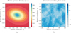 |
Figure 7 Example of a generated two-dimensional random phase screen (b) using the anisotropic power spectral density Fδφ (a). Pictures show only the central portion of the MPS grids in spatial and reciprocal spatial domains. The grid spacings of plots (a) and (b) are Δκx = Δκy = 2.5 × 10⁻³ m−1 and Δx = Δy = 9.7 m, respectively. The number of the shown grid vertices in plot (b) is reduced for a better visibility. The anisotropy coefficients are: |

 |
Figure 8 (a) Simulated phase structure functions are compared with the theoretical von Karman models for isotropic and anisotropic random medium cases. The cross-section along one spatial dimension of this function is shown for convenience. (b) Geometry of multiple phase screens simulation method. |
We now turn to the multiple phase screen (MPS) simulation algorithm (Knepp, 1983; Grimault, 1998; Knepp & Nickisch, 2009). The idea of MPS simulations is based on the split-step method proposed in Refs. (Hardin et al., 1973; Tappert & Hardin, 1975) and mentioned already in Section 2. The basic idea is that the solution of the paraxial wave equation (6) can be modeled as a result of propagation over a set of successive regions filled with the vacuum. These free-space regions are considered to be separated by random phase changing screens in such a way that each phase screen redefines the initial conditions for the vacuum propagation in the region between this screen and the next sequential screen. The solution of the free-space wave equation is obtained by solving the corresponding equation in the Fourier domain and the subsequent application of the inverse Fourier transformation into the spatial domain. The FFT algorithm is used to perform these Fourier transformations.
Let us look at this procedure in some detail. We chose the location of the source at  and again align the z axis along the propagation direction. The position of the jth phase screen we specify to be at
  with
with  and
and  , with
  being the number of phase screens. The electromagnetic wave propagation is given by the paraxial equation (6) which we split in a vacuum propagation part and the part corresponding to propagation in the infinitely thin random phase screen:
![Mathematical equation: $$ 2{ik}\frac{\mathrm{\partial }{u}_{\mathrm{vac}}}{\mathrm{\partial }z}+{\Delta }_{\perp }{u}_{\mathrm{vac}}=0,\enspace \hspace{1em}z\in [{z}_0,{z}_1+\delta {z}_1/2)\cup ({z}_1+\delta {z}_1/2,{z}_2+\delta {z}_2/2)\cup...\cup ({z}_l+\delta {z}_l/2,{z}_r], $$](/articles/swsc/full_html/2022/01/swsc210095/swsc210095-eq234.gif) (72)
(72) (73)where
  is the distance from the receiver to the transmitter and indices “vac” and “med” refer to the vacuum and infinitely thin medium propagation parts, respectively. The geometry of the MPS simulation is summarized in Figure 8b. We now solve the wave equation (72) for propagation in a vacuum with
  in order to find the field at the end of this interval
![Mathematical equation: $$ {u}_{\mathrm{vac}}({\mathbf{r}}_{\perp },{z}_{j+1}+\delta {z}_{j+1}/2)=\int {\mathop{u}\limits^\tilde}_{\mathrm{med}}({\mathbf{\kappa }}_{\perp },{z}_j+\delta {z}_j/2)\mathrm{exp}\left[\frac{i{\kappa }_{\perp }^2}{4k}(\delta {z}_j+\delta {z}_{j+1})\right]{e}^{i{\mathbf{r}}_{\perp }\cdot {\mathbf{\kappa }}_{\perp }}{\mathrm{d}}^2{\mathbf{\kappa }}_{\perp }, $$](/articles/swsc/full_html/2022/01/swsc210095/swsc210095-eq238.gif) (74)where
(74)where  is the Fourier image of the field amplitude formed at the ith phase screen. Here we have also used the identity
  . Similar expressions to (74) are obtained for the end intervals
  and
and ![Mathematical equation: $ ({z}_l+\delta {z}_l/2,{z}_r]$](/articles/swsc/full_html/2022/01/swsc210095/swsc210095-eq243.gif) with appropriate expressions for
with appropriate expressions for  . The boundary condition for the ith screen,
  , in equation (74) is found in turn by taking the Fourier transform of the solution of equation (73) at
  , that is
![Mathematical equation: $$ \begin{array}{c}{\mathop{u}\limits^\tilde}_{\mathrm{med}}({\mathbf{\kappa }}_{\perp },{z}_j+\delta {z}_j/2)=\frac{1}{(2\pi {)}^2}\int {u}_{\mathrm{vac}}({\mathbf{r}}_{\perp },{z}_j)\mathrm{exp}\left({ik}{\int }_{{z}_j}^{{z}_j+\delta {z}_j} {\delta n}({\mathbf{r}}_{\perp },{z}^\mathrm{\prime})\mathrm{d}{z}^\mathrm{\prime}\right){e}^{-i{\mathbf{\kappa }}_{\perp }\cdot {\mathbf{r}}_{\perp }}{\mathrm{d}}^2{\mathbf{r}}_{\perp }\\ \equiv \frac{1}{(2\pi {)}^2}\int {u}_{\mathrm{vac}}({\mathbf{r}}_{\perp },{z}_j+\delta {z}_j/2)\mathrm{exp}\left[{i\delta \phi }({\mathbf{r}}_{\perp },{z}_j+\delta {z}_j/2)\right]{e}^{-i{\mathbf{\kappa }}_{\perp }\cdot {\mathbf{r}}_{\perp }}{\mathrm{d}}^2{\mathbf{r}}_{\perp },\end{array} $$](/articles/swsc/full_html/2022/01/swsc210095/swsc210095-eq247.gif) (75)where in the last line we have used the assumption that the screen is infinitely thin.
(75)where in the last line we have used the assumption that the screen is infinitely thin.
The solutions (74) and (75) show that the field at  is determined by the field formed by the phase screen at
  propagating the distance
  in the vacuum behind this screen. Similarly, the field in
  is determined by the field generated by the
  -th phase screen propagating the distance
  in the vacuum. Thus the field at the given location can be traced backward by such a split-step procedure up to the source of the electromagnetic wave. These steps in solving the paraxial wave equation can be easily rewritten in the discrete form when we define the variables
  and
and  on the grids defined above. Equation (74) then reads as
![Mathematical equation: $$ {u}_{\mathrm{vac}}(m,n,j+1)=\mathrm{FF}{\mathrm{T}}^{-1}\left({\mathop{u}\limits^\tilde}_{\mathrm{med}}({m}^\mathrm{\prime},{n}^\mathrm{\prime},j)\mathrm{exp}\left\{i\frac{{\pi }^2}{k}(\delta {z}_j+\delta {z}_{j+1})\times \left[{\left(\frac{{m}^\mathrm{\prime}}{{L}_x}\right)}^2+{\left(\frac{{n}^\mathrm{\prime}}{{L}_y}\right)}^2\right]\right\}\right), $$](/articles/swsc/full_html/2022/01/swsc210095/swsc210095-eq256.gif) (76)where
(76)where![Mathematical equation: $$ {\mathop{u}\limits^\tilde}_{\mathrm{med}}({m}^\mathrm{\prime},{n}^\mathrm{\prime},j)=\mathrm{FFT}({u}_{\mathrm{vac}}(m,n,j)\mathrm{exp}[{i\delta \phi }(m,n,j)]) $$](/articles/swsc/full_html/2022/01/swsc210095/swsc210095-eq257.gif) (77)follows from equation (75). Here FFT and
(77)follows from equation (75). Here FFT and  are operations of direct and inverse fast Fourier transform, respectively. The phase fluctuation defined on the grid for i-th phase screen,
  , is given by equation (71). By iterating the procedure of the field calculation given in equations (76), (77) over all phase screens, the transmitted field at the receiver site
  can be finally obtained for the specified initial field at
  .
.
The moments of the electromagnetic field required for intensity scintillation index calculations, and the variance of phase fluctuations at the receiver, i.e., phase scintillation index, are obtained by the following procedure. Firstly, the propagation through the set of phase screens is simulated multiple times. For each simulation run the phase screens are generated from scratch. Secondly, the values of transmitted amplitude and phase are collected and used to construct such quantities as the intensity, squared intensity, and squared phase. Finally, the obtained quantities are then averaged over an ensemble of simulation runs and the corresponding scintillation indices are calculated.
We conclude this section by noting that the outlined method of phase screen generation based on the FFT algorithm is not the only possible approach. This method is most commonly used and allows one to generate phase screens with given statistical properties. One should point out that the accuracy and consistency of the FFT method have a close relationship with the number of points in the reciprocal spatial domain at which the PSD is sampled. The insufficient number of sample points may result in the introduction of unphysical artifacts and aliasing effects. Some strategies and algorithms for choosing the optimal sample points, grid spacings, or forms of computational meshes are discussed in detail in Knepp (1983), Lane et al. (1992), Schmidt (2010), Burckel & Gray (2013), Jia et al. (2015). They are based primarily on the use of the above-mentioned Nyquist criterion, on the proper estimate of the receiver region of interest, or on the addition of low-frequency information using subharmonics. The correct reconstruction of the phase structure function could serve as a marker that the sampling grid is chosen properly, cf. Figure 8a. In this respect, the alternative phase screen generated approaches that do not require additional checks might be of interest for the simulation of ionospheric scintillation. We mention here the Zernike polynomial-based phase screen generation method (Roddier, 1990; Carbillet & Riccardi, 2010), the random midpoint displacement-based fractal method (Zhai et al., 2015), the multiscale method (Beghi et al., 2011) or the method based on local principal component analysis (Beghi et al., 2013).
6.2 Example of multiple phase screen simulations: the GISM model
As an illustration of the MPS algorithm, we will discuss the Global Ionospheric Scintillation Model (GISM) (Béniguel, 2002; Béniguel & Hamel, 2011; Béniguel, 2019). The background ionospheric model for the GISM is the NeQuick 2 model (Hochegger et al., 2000; Nava et al., 2008), which provides the value of electron density for a specified spatial point in the ionosphere. The refractive effects due to propagation in the ionosphere are accounted for by the ray-tracing algorithm incorporated in the GISM. Thus, in general cases, the propagation path is not a straight line but rather a complex ray curve consisting of multiple segments. The number of segments and the length of each segment are determined adaptively by the ray-tracing algorithm on the basis of the relative position of the transmitter and the receiver. The phase screens are positioned along such a signal ray so that the screens are concentrated at the maximum of the F layer slant profile determined along the ray. The number,  , and spacings
  , between phase screens are also determined adaptively.
The generation of phase screens in the GISM is based on the von Karman spectrum,  for refractive index fluctuations, cf. equation (22). The strength of fluctuations in the spectrum for jth screen, i.e. the quantity
  , is determined by assuming that the electron density has a constant level of fluctuations
  . This fluctuation level is assumed to be the same for all phase screens, while the mean electron density,
  , varies in accordance with the NeQuick model.
The multiple phase screen simulation within the GISM is organized according to the procedure discussed in detail in Section 6.1. In situations when the anisotropy of irregularities does not sufficiently influence scintillation strength, the multiple phase screens are generated along only one spatial coordinate. Such a simplification considerably saves computational resources and results in MPS with one-dimensional phase screens. In this case, the random phase is generated on a one-dimensional grid, such that it can be written as a one-dimensional discrete Fourier transform (78)where L is the screen size and the one-dimensional spectral function
  is related to the corresponding function for refractive index fluctuations (22) as
  . Analogous equations are obtained for the field amplitudes
  and
and  .
.
For a specified communication scenario, e.g. for orbiting satellite-ground or satellite-satellite links, the GISM outputs a table with information on the coordinates of the transmitter, the RMS value of intensity, and phase scintillation indices, and their margins. The latter gives the information on the probability for an occurrence of calculated scintillation indices. We also mention that the current version of the GISM is optimized for a calculation of the scintillation indices in low latitude regions. Some examples of modeled scintillation indices obtained with the GISM are shown in Figure 9. In particular, Figure 9 (a) shows the global map of the total electron content at 20:00 UT on 15th October 2015. The global distribution of the post-sunset intensity scintillation index is shown in (b). The examples of scintillation sky-maps for the observer in Douala/Cameroon ( N,
N,  E) are shown in (c) and (d) for S4 and
  , respectively. One can clearly see that the scintillation level increases with the increase of the zenith angle if the line of sight is toward the direction where the total electron content is high.
 |
Figure 9 Examples of scintillation plots generated with the GISM. The total electron content values in TEC units calculated by the NeQuick2 background ionospheric model for 15 October 2015 at 20:00 UT (a). The corresponding post sunset distribution of vertical S4 index shown on a globe for signal at the L band (b). The sky-maps as functions of zenith and azimuth angles for: (c) intensity scintillation index S4, (d) phase scintillation index σS. The location of the ground observer is indicated by a star on (b). |
7 Conclusions
The theoretical methods for modeling ionospheric scintillation phenomena have reached the state of maturity during the last several decades. This progress is connected with the development of sophisticated numerical techniques based on the formalism of phase screens. A set of phase screens effectively describes the action of random ionospheric disturbances on propagating electromagnetic waves. Combining free space propagation together with the transmission through phase screens, one can solve the wave equation for wave amplitude as well as infer the corresponding random phase increments. Finally, the scintillation indices of phase and amplitude are obtained by accumulating statistics of simulated intensity and phase fluctuations of the transmitted wave.
The present article reviews these developments in some detail. The emphasis has been placed on the basic concepts, methods, and approximations of ionospheric scintillation modeling based on phase screen formalism. The most important concept of such modeling is that we can simulate the random ionospheric medium only in terms of statistical quantities, e.g. its structure functions and the power spectral densities for electron density (refractive index) fluctuations. The complexity of such a random medium is evident by inspecting the empirical spectra of electron density fluctuations. These spectra show the power-law dependence on spatial frequencies, i.e. quantities that are proportional to reciprocal scales of irregularities causing scintillation. The power-law signifies that the continuum of various scales is involved in the random modulation of amplitude and phase of the transmitting signal. Accounting for the scattering of signal waves at each such scale would be too complex, and this fact makes the statistical approach the most useful and central in scintillation modeling. The article reviews several popular models of power spectral densities such as Gaussian, von Karman, Shkarofsky, and two-component spectra.
As the ionospheric irregularities tend to align along the geomagnetic field lines, these spectra in general, exhibit anisotropy. A standard approximation is that such field-aligned irregularities are characterized by an ellipsoidal form for a surface of constant autocorrelation of electron density fluctuations. For realistic scintillation modeling, it is important to know the parameter set of the specified spectral model, i.e., the axial ratios of the correlation ellipsoid, geometric parameters of its position relative to the communication link, the value of the spectral index, the strength of scattering structures, the outer scale of the medium, etc. We review the dependence of scintillation indices on these parameters. In particular, in the case of weak scattering, it is possible to establish such dependencies in analytic form. We have skipped, however, a detailed discussion of the morphology of ionospheric irregularity parameters.
The objective of discussing some key ideas in ionospheric scintillation modeling has led to the omission of several aspects. Scintillation phenomena should be treated in a specified operational context. This means that depending on the type of the technical system, measuring or detecting apparatus, infrastructure object of interest, etc., only specific aspects of scintillation-related disturbances gain their importance. Depending on the type of particular infrastructure element, the measurement device, or signal postprocessing algorithms, the naturally occurring random fluctuations of phase and amplitude may be partially mitigated or even enhanced. For example, GNSS choke ring antennas are designed to optimally reduce multipath effects while tracking low-elevation satellite signals, while the postprocessing of signals from satellites performs the detrending of geometric factors due to orbital motion. In reflectometric applications at large zenith angles, the receiver detects the multipath contributions that might enhance the scintillation levels. In SAR imaging applications, the signal crosses the random ionospheric medium two times: while propagating in the forward direction as well as after the reflecting from the ground. Moreover, part of the signal can be backscattered and contribute to the ambient noise detected by an antenna. Thus, one expects the enhancement of scintillation due to the specifics of SAR observations. As we can see, all these applications have their own specifics and scintillation indices should be calculated consistently and in agreement with each use case or user requirement under consideration. An example of such case-specific scintillation products could serve the generation of synthetic scintillation data sets Humphreys et al. (2009); Ghafoori & Skone (2014); Rino et al. (2018). Still, these specific products are based on the theoretical foundations of scintillation modeling presented in this article.
Due to practical importance the scintillation forecast remains an important driver for modeling. The climatological models such as WBMOD or GISM are capable of roughly predicting scintillation levels. For example, short-term prediction can be achieved by observing the time series for the model input such as the  solar flux, and predicting their future values, e.g., using the exponential smoothing methods Snyder et al. (2002), the autoregressive and moving average models (Box & Jenkins, 1976), the BATS and TBATS models (De Livera et al., 2012), to name a few. The methods of machine learning and artificial neuronal networks are useful for these demands as well (Qi & Zhang, 2008; Makridakis et al., 2018).
The climatological models tend to provide the averaged indices which might deviate from processes that are highly variable in time and space, which are responsible for scintillation occurrences such as those due to extreme space weather. Therefore, the alternative forecasting approaches have been developed, e.g. based on the direct analysis and assimilation in the climatological models of recorded time series of scintillation indices and other geophysical parameters (Groves et al., 1997; Basu et al., 2002; Rezende et al., 2010; Redmon et al., 2010; McGranaghan et al., 2018) or on the usage of the background physics-based models for electron density (Nugent et al., 2021). In this connection, the space-based high-resolution sensing appears to be critical for accurate characterization and forecasting of scintillation conditions (Kelly et al., 2014).
Several steps might help us to establish reliable and accurate scintillation modeling, monitoring, and prediction services. With every year, more and more data is accumulated, allowing us to gain better insights into ionospheric conditions over solar cycles. The number of satellites and ground stations scanning the Earth ionosphere is also steadily increasing. The combination of data from different remote sensing sources, such as GNSS, SAR, and geostationary satellites, contribute to our better understanding of the volumetric spatial variability of the ionosphere. The development and deployment of the high-resolution electron density monitoring instruments such as EISCAT3D, global ultraviolet imagers (GUVIs), and special sensor ultraviolet spectrographic imagers (SSUSIs), is attractive for an analysis of ionospheric irregularities with an improved spatial and temporal resolution. This, in turn, would facilitate our better understanding of the influence of ionospheric irregularities on radio-wave propagation in the disturbed ionosphere. We expect that the mentioned advances would facilitate the development of scintillation models comparable in their capabilities with the current meteorological weather prediction models.
Acknowledgments
The work was carried out within the programmatic funding of the German Aerospace Center. DV acknowledges C. Baumann for fruitful discussions. The editor thanks Guozhu Li and an anonymous reviewer for their assistance in evaluating this paper.
Stands for WideBand MODel.
Stands for Global Ionospheric Scintillation Model.
Stands for Satellite-beacon Ionospheric-scintillation Global Model of the upper Atmosphere.
The data-driven scintillation climatology code that is the part of the SCIntillation Network Decision Aid.
The splitting process of inhomogeneities in the spatial domain corresponds to the “spectral transfer” or new harmonic generation in the Fourier domain, see e.g., Corrsin (1959). The origin of this effect is rooted in the nonlinearity and the simple analogy from the mathematical analysis (cosξ)2 = [1 + cos(2ξ)]/2, illustrates this effect.

References
- Aarons J. 1982. Global morphology of ionospheric scintillations. Proc IEEE 70: 360–378. https://doi.org/10.1109/PROC.1982.12314. [CrossRef] [Google Scholar]
- Aarons J. 1985. Construction of a model of equatorial scintillation intensity. Radio Sci 20: 397–402. https://doi.org/10.1029/RS020i003p00397. [CrossRef] [Google Scholar]
- Aarons J, MacKenzie E, Bhavnani K. 1980b. High-latitude analytical formulas for scintillation levels. Radio Sci 15: 115–127. https://doi.org/10.1029/RS015i001p00115. [CrossRef] [Google Scholar]
- Abdu MA, Sobral JHA, Batista IS, Rios VH, Medina C. 1998. Equatorial spread-F occurrence statistics in the American longitudes: Diurnal, seasonal and solar cycle variations. Adv Space Res 22: 851–854. https://doi.org/10.1016/S0273-1177(98)00111-2. [CrossRef] [Google Scholar]
- Aquino M, Moore T, Dodson A, Waugh S, Souter J, Rodrigues FS. 2005. Implications of ionospheric scintillation for GNSS users in Northern Europe. J Navigation 58: 241–256. https://doi.org/10.1017/S0373463305003218. [CrossRef] [Google Scholar]
- Banakh VA, Mironov VL. 1979. Phase approximation of the Huygens-Kirchhoff method in problems of space-limited optical-beam propagation in turbulent atmosphere. Opt Lett 4: 259–261. https://doi.org/10.1364/OL.4.000259. [CrossRef] [Google Scholar]
- Basu S, Basu S, Hanson WB. 1981. The role of in situ measurements in scintillation modelling. In: Symposium on the Effect of the Ionosphere on Radiowave Systems. Pap. Nav. Res. Lab, Washington, DC. pp. 4A–8. [Google Scholar]
- Basu S, Basu S, Khan BK. 1976. Model of equatorial scintillation from in situ measurements. Radio Sci 11: 821–832. https://doi.org/10.1029/RS011i010p00821. [CrossRef] [Google Scholar]
- Basu S, Basu S, MacKenzie E, Coley WR, Sharber JR, Hoegy WR. 1990. Plasma structuring by the gradient drift instability at high latitudes and comparison with velocity shear driven processes. J Geophys Res Space Phys 95: 7799–7818. https://doi.org/10.1029/JA095iA06p07799. [CrossRef] [Google Scholar]
- Basu S, Basu S, MacKenzie E, Fougere PF, Coley WR, Maynard NC, Winningham JD, Sugiura M, Hanson WB, Hoegy WR. 1988a. Simultaneous density and electric field fluctuation spectra associated with velocity shears in the auroral oval. J Geophys Res 93: 115–136. https://doi.org/10.1029/JA093iA01p00115. [CrossRef] [Google Scholar]
- Basu S, Basu S, McClure JP, Hanson WB, Whitney HE. 1983. High resolution topside in situ data of electron densities and VHF/GHz scintillations in the equatorial region. J Geophys Res Space Phys 88: 403–415. https://doi.org/10.1029/JA088iA01p00403. [CrossRef] [Google Scholar]
- Basu S, Groves K, Basu S, Sultana P. 2002. Specification and forecasting of scintillations in communication/navigation links: Current status and future plans. J Atm Solar Terr Phys 64: 1745–1754. https://doi.org/10.1016/S1364-6826(02)00124-4. [CrossRef] [Google Scholar]
- Basu S, Kudeki E, Basu S, Valladares CE, Weber EJ, et al. 1996. Scintillations, plasma drifts, and neutral winds in the equatorial ionosphere after sunset. J Geophys Res 101: 26795–26809. https://doi.org/10.1029/96JA00760. [CrossRef] [Google Scholar]
- Basu S, MacKenzie E, Basu S. 1988b. Ionospheric constraints on VHF/UHF communications links during solar maximum and minimum periods. Radio Sci 23: 363–378. https://doi.org/10.1029/RS023i003p00363. [CrossRef] [Google Scholar]
- Basu S, Weber EJ, Bullett TW, Keskinen MJ, MacKenzie E, Doherty P, Sheehan R, Kuenzler H, Ning P, Bongiolatti J. 1998. Characteristics of plasma structuring in the cusp/cleft region at Svalbard. Radio Sci 33: 1885–1899. https://doi.org/10.1029/98RS01597. [CrossRef] [Google Scholar]
- Beghi A, Cenedese A, Masiero A. 2011. Multiscale stochastic approach for phase screens synthesis. Appl Opt 50: 4124–4133. https://doi.org/10.1364/AO.50.004124. [CrossRef] [Google Scholar]
- Beghi A, Cenedese A, Masiero A. 2013. Multiscale phase screen synthesis based on local principal component analysis. Appl Opt 52: 7987–8000. https://doi.org/10.1364/AO.52.007987. [CrossRef] [Google Scholar]
- Belcher DP. 2008. Theoretical limits on SAR imposed by the ionosphere. IET Radar, Sonar and Navigation 2: 435–448. https://doi.org/10.1049/iet-rsn:20070188. [CrossRef] [Google Scholar]
- Béniguel Y. 2002. Global Ionospheric Propagation Model (GIM): A propagation model for scintillations of transmitted signals. Radio Sci 37: 4–1–4–13. https://doi.org/10.1029/2000RS002393. [Google Scholar]
- Béniguel Y. 2019. Ionospheric scintillations: indices and modeling. Radio Sci 54: 618–632. https://doi.org/10.1029/2018RS006655. [Google Scholar]
- Béniguel Y, Hamel P. 2011. A global ionosphere scintillation propagation model for equatorial regions. J Space Weather Space Clim 1: A04. https://doi.org/10.1051/swsc/2011004. [Google Scholar]
- Bhattacharyya A, Rastogi RG. 1985. Amplitude scintillations during the early and late phases of evolution of irregularities in th enighttime equatorial ionosphere. Radio Sci 20: 935–946. https://doi.org/10.1029/RS020i004p00935. [CrossRef] [Google Scholar]
- Bhattacharyya A, Yeh KC, Franke SJ. 1992. Deducing turbulence parameters from transionospheric scintillation measurements. Space Sci Rev 61: 335–386. https://doi.org/10.1007/BF00222311. [CrossRef] [Google Scholar]
- Booker HG. 1958. The use of radio stars to study irregular refraction of radio waves in the ionosphere. Proc IRE 46: 298–314. https://doi.org/10.1109/JRPROC.1958.286791. [CrossRef] [Google Scholar]
- Booker HG, Clemmow PC. 1950. The concept of an angular spectrum of plane waves, and its relation to that of polar diagram and aperture distribution. Proc Inst Elect Engrs Pt III 97: 11–17. https://doi.org/10.1049/pi-3.1950.0002. [Google Scholar]
- Booker HG, Ratcliffe JA, Shinn DH. 1950. Diffraction from an irregular screen with applications to ionospheric problems. Phil Trans Roy Soc A 242: 579–607. https://doi.org/10.1098/rsta.1950.0011. [Google Scholar]
- Bowhill SA. 1961. Statistics of a radio wave diffracted by a random ionosphere. J Res Natl Bur Stand-D 65D: 275–292. [Google Scholar]
- Box GEP, Jenkins GM. 1976. Time series analysis: forecasting and control. Holden-Day, San Francisco. [Google Scholar]
- Bramley EN. 1954. The diffraction of waves by an irregular refracting medium. Proc Roy Soc Lond A 225: 515–518. https://doi.org/10.1098/rspa.1954.0219. [CrossRef] [Google Scholar]
- Bramley EN. 1967. Diffraction of an angular spectrum of waves by a phase-changing screen. J Atm Terr Phys 29: 1–28. https://doi.org/10.1016/0021-9169(67)90155-9. [CrossRef] [Google Scholar]
- Briggs BH. 1968. On the analysis of moving patterns in geophysics – I. Correlation analysis. J Atm Terr Phys 30: 1777–1788. https://doi.org/10.1016/0021-9169(68)90097-4. [CrossRef] [Google Scholar]
- Briggs BH. 1984. The analysis of spaced sensor records by correlation techniques. In: Middle atmosphere program. Handbook for MAP, vol 13, Vincent RE, (Ed.) SCOSTEP Secr. Univ. of Ill, Urbana. pp. 166–186. [Google Scholar]
- Briggs BH, Parkin IA. 1963. On the variation of radio star and satellite scintillations with zenith angle. J Atm Terr Phys 25: 339–366. https://doi.org/10.1016/0021-9169(63)90150-8. [CrossRef] [Google Scholar]
- Burckel WP, Gray RN. 2013. Turbulence phase screens based on polar-logarithmic spectral sampling. Appl Opt 52: 4672–4680. https://doi.org/10.1364/AO.52.004672. [CrossRef] [Google Scholar]
- Butler HE. 1951. Observations of stellar scintillation. Proc IRE 54: 321–340. https://www.jstor.org/stable/20488540. [Google Scholar]
- Camps A, Barbosa J, Juan M, Blanch E, Altadill D, González G, Vazquez G, Riba J, Orús R. 2017. Improved modelling of ionospheric disturbances for remote sensing and navigation. In: 2017 IEEE International Geoscience and Remote Sensing Symposium (IGARSS). pp. 2682–2685. https://doi.org/10.1109/IGARSS.2017.8127548. [CrossRef] [Google Scholar]
- Camps A, Park H, Foti G, Gommenginger C. 2016. Ionospheric effects in GNSS-reflectometry from space. IEEE J Sel Top Appl Earth Obs Remote Sens 9: 5851–5861. https://doi.org/10.1109/JSTARS.2016.2612542. [CrossRef] [Google Scholar]
- Carbillet M, Riccardi A. 2010. Numerical modeling of atmospherically perturbed phase screens: New solutions for classical fast Fourier transform and Zernike methods. Appl Opt 49: G47–G52. https://doi.org/10.1364/AO.49.000G47. [CrossRef] [Google Scholar]
- Carlson HC, Pedersen T, Basu S, Keskinen M, Moen J. 2007. Case for a new process, not mechanism, for cusp irregularity production. J Geophys Res Space Phys 112: A11, 304. https://doi.org/10.1029/2007JA012384. [Google Scholar]
- Carrano CS, Groves KM, Caton RG. 2012. Simulating the impacts of ionospheric scintillation on L band SAR image formation. Radio Sci 47: RS0L20. https://doi.org/10.1029/2011RS004956. [Google Scholar]
- Carrano CS, Groves KM, Caton RG, Rino CL, Straus PR. 2011. Multiple phase screen modeling of ionospheric scintillation along radio occultation raypaths. Radio Sci 46: RS0D07. https://doi.org/10.1029/2010RS004591. [CrossRef] [Google Scholar]
- Carrano CS, Rino CL. 2015. A theory of scintillation for two-component power law irregularity spectra: Overview and numerical results. Radio Sci 51: 789–813. https://doi.org/10.1002/2015RS005903. [Google Scholar]
- Chen S-P, Bilitza D, Liu J-Y, Caton R, Chang LC, Yeh W-H. 2017. An empirical model of L-band scintillation S4 index constructed by using FORMOSAT-3/COSMIC data. Adv Space Res 60: 1015–1028. https://doi.org/10.1016/j.asr.2017.05.031. [CrossRef] [Google Scholar]
- Cho JYN, Kelley MC. 1993. Polar mesosphere summer radar echoes: Observations and current theories. Rev Geophys 31: 243–265. https://doi.org/10.1029/93RG01535. [CrossRef] [Google Scholar]
- Clifford SF. 1978. The classical theory of wave propagation in a turbulent medium. In: Laser beam propagation in the atmosphere. Strohbehn JW (Ed.) Springer-Verlag, Berlin. pp. 9–43. [CrossRef] [Google Scholar]
- Clifford SF, Yura HT. 1974. Equivalence of two theories of strong optical scintillation. J Opt Soc Am 64: 1641–1644. https://doi.org/10.1364/JOSA.64.001641. [CrossRef] [Google Scholar]
- Conker RS, El-Arini MB, Hegarty CJ, Hsiao T. 2003. Modeling the effects of ionospheric scintillation on GPS/Satellite-Based Augmentation System availability. Radio Sci 38: 1–1–1–23. https://doi.org/10.1029/2000RS002604. [Google Scholar]
- Consolini G, De Michelis P, Alberti T, Coco I, Giannattasio F, Tozzi R, Carbone V. 2000. Intermittency and passive scalar nature of electron density fluctuations in the high-latitude ionosphere at Swarm altitude. Geophys Res Lett 47: e2020GL089628. https://doi.org/10.1029/2020GL089628. [Google Scholar]
- Cooley JW, Tukey JW. 1965. An algorithm for the machine calculation of complex Fourier series. Math Comput 19: 297–301. https://doi.org/10.1090/S0025-5718-1965-0178586-1. [CrossRef] [Google Scholar]
- Corrsin S. 1959. Outline of some topics in homogeneous turbulent flow. J Geophys Res 64: 2134–2150. https://doi.org/10.1029/JZ064i012p02134. [CrossRef] [Google Scholar]
- Costa E, Fougere PF, Basu S. 1988. Cross-correlation analysis and interpretation of spaced-receiver measurements. Radio Sci 23: 141–162. https://doi.org/10.1029/RS023i002p00141. [CrossRef] [Google Scholar]
- Crane RK. 1976. Spectra of ionospheric scintillation. J Geophys Res 81: 2041–2050. https://doi.org/10.1029/JA081i013p02041. [CrossRef] [Google Scholar]
- Crane RK. 1977. Ionospheric scintillation. Proc IEEE 65: 180–199. https://doi.org/10.1109/PROC.1977.10456. [CrossRef] [Google Scholar]
- Davidson PA. 2004. Turbulence. An introduction for scientists and engineers. Oxford University Press, Oxford. [Google Scholar]
- De Livera AM, Hyndman RJ, Snyder RD. 2012. Forecasting time series with complex seasonal patterns using exponential smoothing. J Am Stat Assoc 106: 1513–1527. https://doi.org/10.1198/jasa.2011.tm09771. [CrossRef] [Google Scholar]
- De Michelis P, Pignalberi A, Consolini G, Coco I, Tozzi R, Pezzopane M, Giannattasio F, Balasis G. 2020. On the 2015 St. Patrick’s storm turbulent state of the ionosphere: hints from the Swarm mission. J Geophys Res Space Phys 125: e2020JA027934. https://doi.org/10.1029/2020JA027934. [CrossRef] [Google Scholar]
- Deshpande KB, Bust GS, Clauer CR, Rino CL, Carrano CS. 2014. Satellite-beacon Ionospheric-scintillation Global Model of the upper Atmosphere (SIGMA) I: High-latitude sensitivity study of the model parameters. J Geophys Res Space Phys 119: 4026–4043. https://doi.org/10.1002/2013JA019699. [CrossRef] [Google Scholar]
- Deshpande KB, Bust GS, Clauer CR, Scales WA, Frissell NA, Ruohoniemi JM, Spogli L, Mitchell C, Weatherwax AT. 2016. Satellite-beacon Ionospheric-scintillation Global Model of the upper Atmosphere (SIGMA) II: Inverse modeling with high-latitude observations to deduce irregularity physics. J Geophys Res Space Phys 121: 9188–9203. https://doi.org/10.1002/2016JA022943. [CrossRef] [Google Scholar]
- Deshpande KB, Zettergren MD. 2019. Satellite-Beacon Ionospheric-Scintillation Global Model of the upper Atmosphere (SIGMA) III: Scintillation simulation using a physics-based plasma model. Geophys Res Lett 46: 4564–4572. https://doi.org/10.1029/2019GL082576. [CrossRef] [Google Scholar]
- Dyrud L, Krane B, Oppenheim M, Pécseli HL, Trulsen J, Wernik AW. 2008. Structure functions and intermittency in ionospheric plasma turbulence. Nonlin Processes Geophys 15: 847–862. https://doi.org/10.5194/npg-15-847-2008. [CrossRef] [Google Scholar]
- Ellison MA, Seddon H. 1952. Some experiments on the scintillation of stars and planets. MNRAS 112: 73–87. https://doi.org/10.1093/mnras/112.1.73. [CrossRef] [Google Scholar]
- Fante RL. 1975a. Electromagnetic beam propagation in turbulent medium. Proc IEEE 63: 1669–1692. https://doi.org/10.1109/PROC.1975.10035. [CrossRef] [Google Scholar]
- Fante RL. 1975b. Electric field spectrum and intensity covariance of a wave in a random medium. Radio Sci 10: 77–85. https://doi.org/10.1029/RS010i001p00077. [CrossRef] [Google Scholar]
- Fejer JA. 1953. The diffraction of waves in passing through an irregular refracting medium. Proc Roy Soc Lond A 220: 455–471. https://doi.org/10.1098/rspa.1953.0199. [CrossRef] [Google Scholar]
- Forte B, Radicella SM. 2004. Geometrical control of scintillation indices: What happens for GPS satellitess. Radio Sci 39: RS5014. https://doi.org/10.1029/2002RS002852. [Google Scholar]
- Franke SJ, Liu CH. 1983. Observations and modeling of multi-frequency VHF and GHz scintillations in the equatorial region. J Geophys Res 88: 7075–7085. https://doi.org/10.1029/JA088iA09p07075. [CrossRef] [Google Scholar]
- Franke SJ, Liu CH. 1985. Modeling of equatorial multifrequency scintillation. Radio Sci 20: 403–415. https://doi.org/10.1029/RS020i003p00403. [CrossRef] [Google Scholar]
- Franke SJ, Liu CH, Fang DJ. 1984. Multifrequency study of ionospheric scintillation at Ascension Island. Radio Sci 19: 695–706. https://doi.org/10.1029/RS019i003p00695. [CrossRef] [Google Scholar]
- Fremouw EJ. 1980a. Geometrical control of the ratio of intensity and phase scintillation indices. J Atm Terr Phys 42: 775–782. https://doi.org/10.1016/0021-9169(80)90080-X. [CrossRef] [Google Scholar]
- Fremouw EJ, Larsinger JM. 1981. Recent high-latitude improvements in a computer-based scintillation model. In: Effect of the ionosphere on radiowave systems. Goodman JM, Clarke FD, Aarons J (Eds.) Naval Research Lab, Washington DC. pp. 141–154. [Google Scholar]
- Fremouw EJ, Rino CL. 1973. An empirical model for average F: layer scintillation at VHF/UHF. Radio Sci 8: 213–222. https://doi.org/10.1029/RS008i003p00213. [CrossRef] [Google Scholar]
- Fremouw EJ, Secan JA. 1984. Modeling and scientific application of scintillation results. Radio Sci 19: 687–694. https://doi.org/10.1029/RS019i003p00687. [CrossRef] [Google Scholar]
- Ghafoori F, Skone S. 2014. Impact of equatorial ionospheric irregularities on GNSS receivers using real and synthetic scintillation signals. Radio Sci 50: 294–317. https://doi.org/10.1002/2014RS005513. [Google Scholar]
- Gochelashvily KS, Shishov VI. 1975. Saturation of laser irradiance fluctuations beyond a turbulent layer. Opt Quant Electron 7: 524–536. https://doi.org/10.1007/BF00619331. [CrossRef] [Google Scholar]
- Gondarenko NA, Guzdar PN. 2004. Plasma patch structuring by the nonlinear evolution of the gradient drift instability in the high-latitude ionosphere. J Geophys Res Space Phys 109(A09): 301. https://doi.org/10.1029/2004JA010504. [CrossRef] [Google Scholar]
- Gondarenko NA, Guzdar PN. 2006. Nonlinear three-dimensional simulations of mesoscale structuring bymultiple drives in high-latitude plasma patches. J Geophys Res 111(A08): 302. https://doi.org/10.1029/2006JA011701. [Google Scholar]
- Gray AL, Mattar KE, Sofko G. 2000. Influence of ionospheric electron density fluctuations on satellite radar interferometry. Geophys Res Lett 27: 1451–1454. https://doi.org/10.1029/2000GL000016. [CrossRef] [Google Scholar]
- Grimault C. 1998. A multiple phase screen technique for electromagnetic wave propagation through random ionospheric irregularities. Radio Sci 33: 595–605. https://doi.org/10.1029/97RS03552. [CrossRef] [Google Scholar]
- Groves KM, Basu S, Weber EJ, Smitham M, Kuenzler H, et al. 1997. Equatorial scintillation and system support. Radio Sci 32: 2047–2064. https://doi.org/10.1029/97RS00836. [CrossRef] [Google Scholar]
- Guio P, Pécseli HL. 2021. The impact of turbulence on the ionosphere and magnetosphere. Front Astron Space Sci 7(573): 746. https://doi.org/10.3389/fspas.2020.573746. [CrossRef] [Google Scholar]
- Guo K, Zhao Y, Liu Y, Wang J, Zhang C, Zhu Y. 2017. Study of ionospheric scintillation characteristics in Australia with GNSS during 2011–2015. Adv Space Res 59: 2909–2922. https://doi.org/10.1016/j.asr.2017.03.007. [CrossRef] [Google Scholar]
- Gurvich AS, Tatarskii VI. 1975. Coherence and intensity fluctuations of light in the turbulent atmosphere. Radio Sci 10: 3–14. https://doi.org/10.1029/RS010i001p00003. [CrossRef] [Google Scholar]
- Hardin RH, Tappert FD, Whippany NJ. 1973. Applications of the split-step Fourier method to the numerical solution of nonlinear and variable coefficient wave equations. SIAM Rev 15: 423. [Google Scholar]
- Hewish A. 1951. The diffraction of radio waves in passing through a phase-changing ionosphere. Proc Roy Soc A 209: 81–96. https://doi.org/10.1098/rspa.1951.0189. [Google Scholar]
- Hinson D. 1986. Strong scintillations during atmospheric occultations: Theoretical intensity spectra. Radio Sci 21: 257–270. https://doi.org/10.1029/RS021i002p00257. [CrossRef] [Google Scholar]
- Hinson DP. 1984. Magnetic field orientations in Saturn’s upper ionosphere inferred from Voyager radio occultations. J Geophys Res Space Phys 89: 65–73. https://doi.org/10.1029/JA089iA01p00065. [CrossRef] [Google Scholar]
- Hinson DP, Tyler GL. 1982. Spatial irregularities in Jupiter’s upper ionosphere observed by Voyager radio occultations. J Geophys Res Space Phys 87: 5275–5289. https://doi.org/10.1029/JA087iA07p05275. [CrossRef] [Google Scholar]
- Hochegger G, Nava B, Radicella S, Leitinger R. 2000. A family of ionospheric models for different uses. Phys Chem Earth (C) 25: 307–310. https://doi.org/10.1016/S1464-1917(00)00022-2. [CrossRef] [Google Scholar]
- Horvath I, Crozier S. 2007. Software developed for obtaining GPS-derived total electron content values. Radio Sci 42: RS2002. https://doi.org/10.1029/2006RS003452. [Google Scholar]
- Huang CS, de La Beaujardiere O, Roddy PA, Hunton DE, Liu JY, Chen SP. 2014a. Occurrence probability and amplitude of equatorial ionospheric irregularities associated with plasma bubbles during low and moderate solar activities (2008–2012). J Geophys Res Space Phys 119: 1186–1199. https://doi.org/10.1002/2013JA019212. [CrossRef] [Google Scholar]
- Humphreys TE, Psiaki ML, Hinks JC, O’Hanlon B, Kintner PM. 2009. Simulating ionosphere-induced scintillation for testing GPS receiver phase tracking loops. IEEE J Selected Topics Signal Proc 3: 707–715. https://doi.org/10.1109/JSTSP.2009.2024130. [CrossRef] [Google Scholar]
- Hysell DI, Kelley MC, Swartz WE, Pfaff RF, Swenson CM. 1994a. Steepened structures in equatorial spread F: 1. New observations. J Geophys Res 99: 8827–8840. https://doi.org/10.1029/93JA02961. [CrossRef] [Google Scholar]
- Hysell DI, Seyler CE, Kelley MC. 1994b. Steepened structures in equatorial spread F: 2. Theory. J Geophys Res 99: 8841–8850. https://doi.org/10.1029/93JA02960. [CrossRef] [Google Scholar]
- Hysell DL, Kelley MC. 1997. Decaying equatorial F region plasma depletions. J Geophys Res 102: 20007–20017. https://doi.org/10.1029/97JA01725. [CrossRef] [Google Scholar]
- Hysell DL, Shume EB. 2002. Electrostatic plasma turbulence in the topside equatorial F region ionosphere. J Geophys Res 107: SIA1-1–SIA1-12. https://doi.org/10.1029/2001JA000227. [Google Scholar]
- Inhester B, Ulwick JC, Cho J, Kelley MC, Schmidt G. 1990. Consistency of rocket and radar electron density observations: implication about the anisotropy of mesospheric turbulence. J Atm Terr Phys 52: 855–873. https://doi.org/10.1016/0021-9169(90)90021-E. [CrossRef] [Google Scholar]
- Ishimaru A. 1978. Wave propagation and scattering in random media, vol. 2, Academic Press, New York. [Google Scholar]
- Ishimaru A, Kuga Y, Liu J, Kim Y, Freeman T. 1999. Ionospheric effects on synthetic aperture radar at 100 MHz to 2 GHz. Radio Sci 34: 257–268. https://doi.org/10.1029/1998RS900021. [CrossRef] [Google Scholar]
- Iyer KN, Souza JR, Pathan BM, Abdu MA, Jivani MN, Joshi HP. 2006. A model of equatorial and low latitude VHF scintillation in India. Indian J Radio Space Phys 35: 98–104. [Google Scholar]
- Jeruchim MC, Balaban P, Shanmugan KS. 2000. Simulation of communication systems, 2nd edn. Kluwer Academic Publishers, New York. [CrossRef] [Google Scholar]
- Jia P, Cai D, Wang D, Basden A. 2015. Simulation of atmospheric turbulence phase screen for large telescope and optical interferometer. MNRAS 447: 3467–3474. https://doi.org/10.1093/mnras/stu2655. [CrossRef] [Google Scholar]
- Jiao Y, Morton YT. 2015. Comparison of the effect of high-latitude and equatorial ionospheric scintillation on GPS signals during the maximum of solar cycle 24. Radio Sci 50: 886–903. https://doi.org/10.1002/2015RS005719. [CrossRef] [Google Scholar]
- Jin Y, Miloch WJ, Moen JI, Clausen LBN. 2018. Solar cycle and seasonal variations of the GPS phase scintillation at high latitudes. J Space Weather Space Clim 8: A48. https://doi.org/10.1051/swsc/2018034. [CrossRef] [EDP Sciences] [Google Scholar]
- Jin Y, Moen JI, Spicher A, Oksavik K, Miloch WJ, Clausen LBN, Požoga M, Sato Y. 2019. Simultaneous rocket and scintillation observations of plasma irregularities associated with a reversed flow event in the casp ionosphere. Progr Earth Planet Sci 124: 7098–7111. https://doi.org/10.1029/2019JA026942. [Google Scholar]
- Kelley MC, Baker KD, Ulwick JC, Rino CL, Baron MJ. 1980. Simultaneous rocket probe, scintillation, and incoherent scatter radar observations of irregularities in the auroral zone ionosphere. Radio Sci 15: 491–505. https://doi.org/10.1029/RS015i003p00491. [CrossRef] [Google Scholar]
- Kelley MC, Livingston RC, Rino CL, Tsunoda RT. 1982. The vertical wave number spectrum of topside equatorial spread F: Estimates of backscatter levels and implications for a unified theory. J Geophys Res Space Phys 87: 5217–5221. https://doi.org/10.1029/JA087iA07p05217. [CrossRef] [Google Scholar]
- Kelley MC, Makela JJ, Ledvina BM, Kintner PM. 2002. Observations of equatorial spread-F from Haleakala, Hawaii. Geophys Res Lett 29: 64-1–64–4. https://doi.org/10.1029/2002GL015509. [CrossRef] [Google Scholar]
- Kelley MC, Ott E. 1978. Two-dimensional turbulence in equatorial spread F. J Geophys Res Space Phys 83: 4369–4372. https://doi.org/10.1029/JA083iA09p04369. [CrossRef] [Google Scholar]
- Kelly M, Comberiate JM, Miller ES, Paxton LJ. 2014. Progress toward forecasting of space weather effects on UHF SATCOM after Operation Anaconda. Space Weather 12: 601–611. https://doi.org/10.1002/2014SW001081. [CrossRef] [Google Scholar]
- Keskinen MJ, Mitchell HG, Fedder JA, Satyanarayana P, Zalesak ST, Huba JD. 1988. Nonlinear evolution of the Kelvin-Helmholtz instability in the high-latitude ionosphere. J Geophys Res Space Phys 93: 137–152. https://doi.org/10.1029/JA093iA01p00137. [CrossRef] [Google Scholar]
- Keskinen MJ, Ossakow SL, Chaturvedi PK. 1980. Preliminary report of numerical simulations of intermediate wavelength collisional Rayleigh-Taylor instability in equatorial spread F. J Geophys Res 85: 1775–1778. https://doi.org/10.1029/JA085iA04p01775. [CrossRef] [Google Scholar]
- Kintner PM, Seyler CE. 1985. The status of observations and theory of high latitude ionospheric and magnetospheric plasma turbulence. Space Sci Rev 41: 91–129. https://doi.org/10.1007/BF00241347. [CrossRef] [Google Scholar]
- Kivanç Ö, Heelis RA. 1997. Structures in ionospheric number density and velocity associated with polar cap ionization patches. J Geophys Res Space Phys 102: 307–318. https://doi.org/10.1029/96JA03141. [CrossRef] [Google Scholar]
- Knepp DL. 1983. Multiple phase-screen calculation of the temporal behavior of stochastic waves. Proc IEEE 71: 722–737. https://doi.org/10.1109/PROC.1983.12660. [CrossRef] [Google Scholar]
- Knepp DL, Nickisch LJ. 2009. Multiple phase screen calculation of wide bandwidth propagation. Radio Sci 44: RS0A09. https://doi.org/10.1029/2008RS004054. [Google Scholar]
- Knight M, Finn A. 1998. The effects of ionospheric scintillations on GPS. In: Proceedings of the 11th International Technical Meeting of the Satellite Division of The Institute of Navigation (ION GPS 1998), Nashville, TN. pp. 673–685. [Google Scholar]
- Kolmogorov AN. 1941. The local structure of turbulence in incompressible viscous fluid for very large Raynolds numbers. Dokl Akad Nauk SSSR 30: 299. https://doi.org/10.1098/rspa.1991.0075. [Google Scholar]
- Kovasznay LSG, Uberoi MS, Corrsin S. 1949. The transformation between one- and three-dimensional power spectra for an isotropic scalar fluctuation field. Phys Rev 76: 1263. https://doi.org/10.1103/PhysRev.76.1263.2. [CrossRef] [Google Scholar]
- Krane B, Pécseli HL, Trulsen J, Primdahl F. 2000. Spectral properties of low-frequency electrostatic waves in the ionospheric E region. J Geophys Res 105: 10585–10601. https://doi.org/10.1029/1999JA900503. [CrossRef] [Google Scholar]
- Kravtsov YA. 1992. Propagation of electromagnetic waves through a turbulent atmosphere. Rep Prog Phys 55: 39–112. https://doi.org/10.1088/0034-4885/55/1/002. [CrossRef] [Google Scholar]
- Kriegel M, Jakowski N, Berdermann J, Sato H, Mogese WM. 2017. Scintillation measurements at Bahir Dar during the high solar activity phase of solar cycle 24. Ann Geophys 35(1): 97–106. https://doi.org/10.5194/angeo-35-97-2017. [CrossRef] [Google Scholar]
- Lane RG, Glindemann A, Dainty JC. 1992. Simulation of a Kolmogorov phase screen. Waves in Random Media 2: 209–224. https://doi.org/10.1088/0959-7174/2/3/003. [CrossRef] [Google Scholar]
- Leitinger R. 2001. Modern aspects of ionospheric propagation research. In: Eleventh International Conference on Antennas and Propagation (IEE Conf. Publ. No. 480). pp. 677–681. https://doi.org/10.1049/cp:20010376. [Google Scholar]
- Liu CH, Wernik AW, Yeh KC, Youakim MY. 1974. Effects of multiple scattering on scintillation of transionospheric radio signals. Radio Sci 9: 599–607. https://doi.org/10.1029/RS009i006p00599. [CrossRef] [Google Scholar]
- Liu CH, Yeh KC. 1978. Pulse propagation in random media. IEEE Trans Antennas Propagat AP-26: 561–566. https://doi.org/10.1109/TAP.1978.1141888. [Google Scholar]
- Liu Y-H, Liu C-H, Su S-Y. 2012. Global and seasonal scintillation morphology in the equatorial region derived from ROCSAT-1 in-situ data. Terr Atmos Ocean Sci 23: 95–106. https://doi.org/10.3319/TAO.2011.06.30.01(AA). [CrossRef] [Google Scholar]
- Ludwig-Barbosa V, Rasch J, Carlstöm A, Pettersson MI, Vu VT. 2020. GNSS radio occultation simulation using multiple phase screen orbit sampling. IEEE Geosci Remote Sensing Lett 17: 1323–1327. https://doi.org/10.1109/LGRS.2019.2944537. [CrossRef] [Google Scholar]
- Mahan AI. 1962. Astronomical refraction – some history and theories. Appl Opt 1: 497–511. https://doi.org/10.1364/AO.1.000497. [CrossRef] [Google Scholar]
- Makridakis S, Spiliotis E, Assimakopoulos V. 2018. Statistical and Machine Learning forecasting methods: Concerns and ways forward. PLoS One 13(e0194): 889. https://doi.org/10.1371/journal.pone.0194889. [Google Scholar]
- Mannix CR, Belcher DP, Cannon PS. 2017. Measurement of ionospheric scintillation parameters from SAR images using corner reflectors. IEEE Trans Geosci Remote Sens 55: 6695–6702. https://doi.org/10.1109/TGRS.2017.2727319. [CrossRef] [Google Scholar]
- McDonald BE, Coffey TP, Ossakow S, Sudan RN. 1974. Preliminary report of numerical simulation of Type 2 irregularities in the equatorial electrojet. J Geophys Res 79: 2551–2554. https://doi.org/10.1029/JA079i016p02551. [CrossRef] [Google Scholar]
- McGranaghan RM, Mannucci AJ, Wilson B, Mattmann CA, Chadwick R. 2018. New capabilities for prediction of high-latitude ionospheric scintillation: A novel approach with machine learning. Space Weather 16: 1817–1846. https://doi.org/10.1029/2018SW002018. [Google Scholar]
- Mercier RP. 1962. Diffraction by a screen causing large random phase fluctuations. Proc Camb Phil Soc A 58: 382–400. https://doi.org/10.1017/S0305004100036586. [CrossRef] [Google Scholar]
- Mikkelsen T, Pécseli HL. 1980. Strong turbulence in partially ionized plasmas. Phys Lett A 77: 159–162. https://doi.org/10.1016/0375-9601(80)90179-6. [CrossRef] [Google Scholar]
- Moorcroft DR, Arima KS. 1972. The shape of the F-region irregularities which produce satellite scintillations – Evidence for axial asymmetry. J Atm Terr Phys 34: 437–450. https://doi.org/10.1016/0021-9169(72)90045-1. [CrossRef] [Google Scholar]
- Moorthy KK, Reddi CR, Murthy BK. 1979. Night-time ionospheric scintillations at the magnetic equator. J Atm Terr Phys 41: 123–134. https://doi.org/10.1016/0021-9169(79)90004-7. [CrossRef] [Google Scholar]
- Muella MTAH, de Paula ER, Monteiro AA. 2013. Ionospheric scintillation and dynamics of Fresnel-scale irregularities in the inner region of the equatorial ionization anomaly. Surv Geophys 34: 233–251. https://doi.org/10.1007/s10712-012-9212-0. [CrossRef] [Google Scholar]
- Muralikrishna P, Vieira LP, Abdu MA. 2007. Spectral features of E- and F-region plasma irregularities as observed by rocket-borne electron density probes from Brazil. Rev Bras Geof 25: 115–128. https://doi.org/10.1590/S0102-261X2007000600014. [Google Scholar]
- Nava B, Coisson P, Radicella SM. 2008. A new version of the NeQuick ionosphere electron density model. J Atm Sol Terr Phys 70: 1856–1862. https://doi.org/10.1016/j.jastp.2008.01.015. [CrossRef] [Google Scholar]
- Nugent LD, Elvidge S, Angling MJ. 2021. Comparison of low-latitude ionospheric scintillation forecasting techniques using a physics-based model. Space Weather 19: e2020SW002 462. https://doi.org/10.1029/2020SW002462. [CrossRef] [Google Scholar]
- Obukhov AM. 1949. Structure of the temperature field in turbulent stream. Izv Akad Nauk SSSR, Geogr Geofiz 13: 58–69. [Google Scholar]
- Obukhov AM. 1953. Effect of weak inhomogeneities in the atmosphere on sound and light propagation. Izv Akad Nauk SSSR Ser Geophys 2: 155–165. [Google Scholar]
- Papoulis A, Pillai S. 2002. Probability, random variables and stochastic processes. McGraw-Hill, New York. [Google Scholar]
- Parkin IA. 1967. The effects of field-aligned ionospheric irregularities on satellite scintillations. J Atm Terr Phys 30: 1135–1142. https://doi.org/10.1016/S0021-9169(68)80003-0. [Google Scholar]
- Patel K, Singh AK, Patel RP, Singh RP. 2009. Characteristics of low latitude ionospheric E-region irregularities linked with daytime VHF scintillations measured from Varanasi. J Earth Syst Sci 118: 721–732. https://doi.org/10.1007/s12040-009-0058-x. [CrossRef] [Google Scholar]
- Prakash S, Gupta SP, Subbaraya BH, Jain CL. 1971a. Electrostatic plasma instabilities in the equatorial electrojet. Nature 233: 56–58. https://doi.org/10.1038/physci233056a0. [CrossRef] [Google Scholar]
- Prakash S, Subbaraya BH, Gupta SP. 1971b. Rocket measurements of ionization irregularities in the equatorial ionosphere at Thumba and identification of plasma instabilities. Indian J Radio Space Phys 1: 72–80. [Google Scholar]
- Priyadarshi S. 2015. A review of ionospheric scintillation models. Surv Geophys 36: 295–324. https://doi.org/10.1007/s10712-015-9319-1. [CrossRef] [Google Scholar]
- Prokhorov AM, Bunkin FV, Gochelashvily KS, Shishov VI. 1975. Laser irradiance propgataion in turbulent media. Proc IEEE 63: 790–811. https://doi.org/10.1109/PROC.1975.9828. [CrossRef] [Google Scholar]
- Qi M, Zhang GP. 2008. Trend time-series modeling and forecasting with neural networks. IEE Trans Neural Netw 19: 808–816. https://doi.org/10.1109/TNN.2007.912308. [CrossRef] [Google Scholar]
- Ratcliffe JA. 1956. Some aspects of diffraction theory and their application to the ionosphere. Rep Prog Phys 19: 188–267. https://doi.org/10.1088/0034-4885/19/1/306. [CrossRef] [Google Scholar]
- Rawer K. 1993. Wave propagation in the ionosphere. Kluwer Academic Publishers, Dordrecht. [CrossRef] [Google Scholar]
- Redmon RJ, Anderson D, Caton R, Bullett T. 2010. A forecasting ionospheric real-time scintillation tool (FIRST). Space Weather 8(S12): 003. https://doi.org/10.1029/2010SW000582. [Google Scholar]
- Retterer JM. 2010. Forecasting low-latitude radio scintillation with 3-D ionospheric plume models: 2. Scintillation calculation. J Geophys Res 115(A03): 307. https://doi.org/10.1029/2008JA013840. [Google Scholar]
- Rezende LFC, de Paula ER, Stephany S, Kantor IJ, Muella MTAH, de Siqueira PM, Correa KS. 2010. Survey and prediction of the ionospheric scintillation using data mining techniques. Space Weather 8: S06D09. https://doi.org/10.1029/2009SW000532. [Google Scholar]
- Rice SO. 1944. Mathematical analysis of random noise. Bell Sys Tech J 23: 282–332. https://doi.org/10.1002/j.1538-7305.1944.tb00874.x. [CrossRef] [Google Scholar]
- Rice SO. 1945. Mathematical analysis of random noise. Bell Sys Tech J 24: 46–156. https://doi.org/10.1002/j.1538-7305.1945.tb00453.x. [CrossRef] [Google Scholar]
- Rickett B. 1977. Interstellar scattering and scintillation of radio waves. Ann Rev Astrophys 15: 479–504. https://doi.org/10.1146/annurev.aa.15.090177.002403. [CrossRef] [Google Scholar]
- Rino C, Breitsch B, Morton Y, Jiao Y, Xu D, Carrano C. 2018. A compact multi-frequency GNSS scintillation model. Navigation 65: 563–569. https://doi.org/10.1002/navi.263. [CrossRef] [Google Scholar]
- Rino CL. 1979a. A power law phase screen model for ionospheric scintillation: 1. Weak scatter. Radio Sci 14: 1135–1145. https://doi.org/10.1029/RS014i006p01135. [CrossRef] [Google Scholar]
- Rino CL. 1979b. A power law phase screen model for ionospheric scintillation: 2. Strong scatter. Radio Sci 14: 1147–1155. https://doi.org/10.1029/RS014i006p01147. [CrossRef] [Google Scholar]
- Rino CL. 1982a. On the application of phase screen models to the interpretation of ionospheric scintillation data. Radio Sci 17: 855–867. https://doi.org/10.1029/RS017i004p00855. [CrossRef] [Google Scholar]
- Rino CL. 2011. The theory of scintillation with applications in remote sensing. Wiley, New Jersey. [CrossRef] [Google Scholar]
- Rino CL, Fremouw EJ. 1977. The angle dependence of singly scattered wavefields. J Atm Terr Phys 39: 859–868. https://doi.org/10.1016/0021-9169(77)90166-0. [CrossRef] [Google Scholar]
- Rino CL, Tsunoda RT, Petriceks J, Livingston RC, Kelley MC, Baker KD. 1981. Simultaneous rocket-borne beacon and in situ measurements of equatorial spread F – Intermediate wavelength results. J Geophys Res 86: 2411–2420. https://doi.org/10.1029/JA086iA04p02411. [CrossRef] [Google Scholar]
- Roddier NA. 1990. Atmospheric wavefront simulation using Zernike polynomials. Opt Eng 29: 1174–1180. https://doi.org/10.1117/12.55712. [CrossRef] [Google Scholar]
- Rogers NC, Quegan S, Kim JS, Papathanassiou KP. 2014. Impacts of ionospheric scintillation on the BIOMASS P-band satellite SAR. IEEE Trans Geosci Remote Sens 52: 1856–1868. https://doi.org/10.1109/TGRS.2013.2255880. [CrossRef] [Google Scholar]
- Rufenach C. 1972. Power-law wavenumber spectrum deduced from ionospheric scintillation observations. J Geophys Res 77: 4761–4772. https://doi.org/10.1029/JA077i025p04761. [CrossRef] [Google Scholar]
- Rumsey VH. 1975. Scintillations due to a concentrated layer with a power-law turbulence spectrum. Radio Sci 10: 107–114. https://doi.org/10.1029/RS010i001p00107. [CrossRef] [Google Scholar]
- Sato H, Kim JS, Otsuka Y, Wrasse CM, de Paula ER, de Souza JR. 2021. L-band synthetic aperture radar observation of ionospheric density irregularities at equatorial plasma depletion region. Geophys Res Lett 48: e2021GL093 541. https://doi.org/10.1029/2021GL093541. [Google Scholar]
- Schmidt J. 2010. Numerical simulation of optical wave propagation with examples in MATLAB. SPIE Press, Bellingham. [CrossRef] [Google Scholar]
- Secan JA, Bussey RM, Fremouw EJ, Basu S. 1995. An improved model of equatorial scintillation. Radio Sci 30: 607–617. https://doi.org/10.1029/94RS03172. [CrossRef] [Google Scholar]
- Secan JA, Bussey RM, Fremouw EJ, Basu S. 1997. High-latitude upgrade to the Wideband ionospheric scintillation model. Radio Sci 32: 1567–1574. https://doi.org/10.1029/97RS00453. [CrossRef] [Google Scholar]
- Shishov VI. 1968. Theory of wave propagation in random media. Radiophys Quant Electr 11: 500–505. https://doi.org/10.1007/BF01033362. [CrossRef] [Google Scholar]
- Shishov VI. 1974. Dependence of the form of the scintillation spectrum on the form of the spectrum of refractive-index inhomogeneities. Communication I. A phase screen. Radiophys Quantum Electron 17: 1287–1292. https://doi.org/10.1007/BF01042029. [CrossRef] [Google Scholar]
- Shishov VI. 1976. Scintillation spectrum as a function of the spectrum of refractive-index irregularities II. Statistically homogeneous medium. Radiophys Quantum Electron 19: 62–68. https://doi.org/10.1007/BF01038410. [CrossRef] [Google Scholar]
- Shishov VI, Tyulbashev SA, Chashei IV, Subaev IA, Lapaev KA. 2010. Interplanetary and ionosphere scintillation monitoring of radio sources ensemble at the solar activity minimum. Solar Phys 265: 277–291. https://doi.org/10.1007/s11207-010-9565-9. [CrossRef] [Google Scholar]
- Shkarofsky IP. 1968. Generalized turbulence space-correlation and wave-number spectrum-function pairs. Can J Phys 46: 2133–2153. https://doi.org/10.1139/p68-562. [CrossRef] [Google Scholar]
- Siefring CL, Bernhardt PA, Koch DE, Galysh IJ. 2011. Using TEC and radio scintillation data from the CITRIS radio beacon receiver to study low and midlatitude ionospheric irregularities. Radio Sci 46: RS0D19. https://doi.org/10.1029/2010RS004585. [CrossRef] [Google Scholar]
- Singleton DG. 1970a. The effect of irregularity shape on radio star and satellite scintillations. J Atm Terr Phys 32: 315–343. https://doi.org/10.1016/0021-9169(70)90005-X. [CrossRef] [Google Scholar]
- Singleton DG. 1970b. Dependence of satellite scintillations on zenith angle and azimuth. J Atm Terr Phys 32: 789–803. https://doi.org/10.1016/0021-9169(70)90029-2. [CrossRef] [Google Scholar]
- Singleton DG. 1973. The dependence of high-latitude ionospheric scintillations on zenith angle and azimuth. J Atm Terr Phys 35: 2253–2265. https://doi.org/10.1016/0021-9169(73)90141-4. [CrossRef] [Google Scholar]
- Singleton DG. 1974. Power spectra of ionospheric scintillations. J Atm Terr Phys 36: 113–133. https://doi.org/10.1016/0021-9169(74)90071-3. [CrossRef] [Google Scholar]
- Snyder R, Koehler A, Ord J. 2002. Forecasting for inventory control with exponential smoothing. Int J Forecast 18: 5–18. https://doi.org/10.1016/S0169-2070(01)00109-1. [CrossRef] [Google Scholar]
- Sokolovskiy SV. 2000. Inversion of radio occulatation amplitude data. Radio Sci 35: 97–105. https://doi.org/10.1029/1999RS002203. [CrossRef] [Google Scholar]
- Souto Fortes LP, Lin T, Lachapelle G. 2015. Effects of the 2012–2013 solar maximum on GNSS signals in Brazil. GPS Solut 19: 309–319. https://doi.org/10.1007/s10291-014-0389-1. [CrossRef] [Google Scholar]
- Spicher A, Miloch WJ, Clausen LBN, Moen JI. 2015. Plasma turbulence and coherent structures in the polar cap observed by the ICI-2 sounding rocket. J Geophys Res Space Phys 120: 10959–10978. https://doi.org/10.1002/2015JA021634. [CrossRef] [Google Scholar]
- Spogli L, Alfonsi L, Franceschi GD, Romano V, Aquino MHO, Dodson A. 2009. Climatology of GPS ionospheric scintillations over high andmid-latitude European regions. Ann Geophys 27: 3429–3437. https://doi.org/10.5194/angeo-27-3429-2009. [CrossRef] [Google Scholar]
- Sreeja V, Aquino M, Elmas ZG. 2011. Impact of ionospheric scintillation on GNSS receiver tracking performance over Latin America: Introducing the concept of tracking jitter variance maps. Space Weather 9(S10): 002. https://doi.org/10.1029/2011SW000707. [CrossRef] [Google Scholar]
- Strangeways HJ, Zernov NN, Gherm VE. 2013. Comparison of four methods for transionospheric scintillation evaluation. Radio Sci 49: 899–909. https://doi.org/10.1002/2014RS005408. [CrossRef] [Google Scholar]
- Strom R, Bo P, Walker M, Rendong N, eds. 2001. Sources and scintillations: Refraction and scattering in radio astronomy IAU Colloquium 182. Springer Science + Business Media, Dordrecht. https://doi.org/10.1007/978-94-010-1001-6. [Google Scholar]
- Tappert FD, Hardin RH. 1975. Computer simulation of long-range ocean acoustic propagation using the parabolic equation method. In: Eight international congress on acoustics, London, 1974, vol. 2, Goldcrest Press, Trowbridge. p. 452. [Google Scholar]
- Tatarski VI. 2016. Wave propagation in a turbulent medium. Dover, New York. [Google Scholar]
- Tatarskii VI. 1971. The effects of the turbulent atmosphere on wave propagation. Israel Program for Scientific Translations, Jerusalem. [Google Scholar]
- Tatarskii VI, Charnotskii MI, Gozani J, Zavorotny VU. 1992. Path integral approach to wave propagation in a random media. Part I: derivations and various formulations. In: Wave propagation in random media (Scintillation). Tatarskii VI, Ishimaru A, Zavorotny VU, (Eds.) SPIE Press, Bellingham. pp. 383–402. [Google Scholar]
- Taylor GI. 1938. The spectrum of turbulence. Proc Royal Soc A 164: 476–490. https://doi.org/10.1098/rspa.1938.0032. [Google Scholar]
- Tennekes H. 1975. Eulerian and Lagrangian time microscales in isotropic turbulence. J Fluid Mech 67: 561–567. https://doi.org/10.1017/S0022112075000468. [CrossRef] [Google Scholar]
- Tsai L-C, Su S-Y, Liu C-H. 2017. Global morphology of ionospheric F-layer scintillationsusing FS3/COSMIC GPS radio occultation data. GPS Solu 21: 1037–1048. https://doi.org/10.1007/s10291-016-0591-4. [CrossRef] [Google Scholar]
- Umeki R, Liu CH, Yeh KC. 1977. Multifrequency spectra of ionospheric amplitude scintillations. Space Phys 82: 2752–2760. https://doi.org/10.1029/JA082i019p02752. [Google Scholar]
- Uscinski BJ. 1978. Use of physical concepts in delaing with problems of multiple scatter. J Atm Terr Phys 40: 1257–1266. https://doi.org/10.1016/0021-9169(78)90076-4. [CrossRef] [Google Scholar]
- Uscinski BJ. 1982. Intensity fluctuations in a multiple scattering medium. Solution of the fourth moment equation. Proc R Soc Lond A 380: 137–169. https://doi.org/10.1098/rspa.1982.0034. [CrossRef] [Google Scholar]
- Uscinski BJ. 1985. Analytical solution of the fourth-moment equation and interpretation as a set of phase screens. J Opt Soc Am A 2: 2077–2091. https://doi.org/10.1364/JOSAA.2.002077. [CrossRef] [Google Scholar]
- van de Kamp M, Cannon PS, Terkildsen M. 2009. Effect of the ionosphere on defocusing of space-based radars. Radio Sci 44: RS1003. https://doi.org/10.1029/2007RS003808. [Google Scholar]
- Voitsekhovich VV. 1995. Outer scale of turbulence: comparison of different models. J Opt Soc Am A 12: 1346–1353. https://doi.org/10.1364/JOSAA.12.001346. [CrossRef] [Google Scholar]
- Wand RH, Evans JV. 1975. Morphology of ionospheric scintillation in the auroral zone. In: Goodman J, (Ed.). Effect of the Ionosphere on Space Systems and Communication, NTIS CSCL 04/1 N75-30714. pp. 76–83. [Google Scholar]
- Weinstock J, Sleeper A. 1972. Nonlinear saturation of “Type I” irregularities in the equatorial electrojet. J Geophys Res 77: 3621–3624. https://doi.org/10.1029/JA077i019p03621. [CrossRef] [Google Scholar]
- Weisbrod S, Anderson LJ. 1959. Simple methods for computing tropospheric and ionospheric refractive effects on radio waves. Proc IRE 47: 1770–1777. https://doi.org/10.1109/JRPROC.1959.287112. [CrossRef] [Google Scholar]
- Wernik AW, Alfonsi L, Materassi M. 2007. Scintillation modeling using in situ data. Radio Sci 42: RS1002. https://doi.org/10.1029/2006RS003512. [Google Scholar]
- Wheelon AD. 2003. Electromagnetic scintillation II. Weak scattering. Cambridge University Press, Cambridge. [CrossRef] [Google Scholar]
- Wheelon AD. 2004. Electromagnetic scintillation I. Geometrical optics. Cambridge University Press, Cambridge. [Google Scholar]
- Yakushkin IG. 1975. Asymptotic calculation of field-intensity fluctuations in a turbulent medium for long paths. Radiophys Quant Electron 18: 1224–1229. https://doi.org/10.1007/BF01037115. [CrossRef] [Google Scholar]
- Yeh KC, Liu C-H. 1982. Radio wave scintillations in the ionosphere. Proc IEEE 70: 324–360. https://doi.org/10.1109/PROC.1982.12313. [CrossRef] [Google Scholar]
- Yokoyama T. 2017b. A review on the numerical simulation of equatorial plasma bubbles toward scintillation evaluation and forecasting. Prog Earth Planet Sci 4: 37. https://doi.org/10.1186/s40645-017-0153-6. [CrossRef] [Google Scholar]
- Yokoyama T, Stolle C. 2017. Low and midlatitude ionospheric plasma density irregularities and their effects on geomagnetic field. Space Sci Rev 206: 495–519. https://doi.org/10.1007/s11214-016-0295-7. [CrossRef] [Google Scholar]
- Young MA, Oppenheim MM, Dimant YS. 2020. The Farley-Buneman spectrum in 2-D and 3-D Particle-in-Cell simulations. J Geophys Res Space Phys 125: e2019JA027 326. https://doi.org/10.1029/2019JA027326. [CrossRef] [Google Scholar]
- Zavorotny VU, Charnotskii MI, Gozani J, Tatarskii VI. 1992. Path integral approach to wave propagation in a random media. Part II: exact formulations and heuristic approximations. In: Wave propagation in random media (Scintillation). Tatarskii VI, Ishimaru A, Zavorotny VU, (Eds.) SPIE Press, Bellingham. pp. 403–421. [Google Scholar]
- Zhai H, Wang B, Zhang J, Dang A. 2015. Fractal phase screen generation algorithm for atmospheric turbulence. Appl Opt 54: 4023–4032. https://doi.org/10.1364/AO.54.004023. [CrossRef] [Google Scholar]
Cite this article as: Vasylyev D, Béniguel Y, Volker W, Kriegel M & Berdermann J, et al. 2022. Modeling of ionospheric scintillation. J. Space Weather Space Clim. 12, 22. https://doi.org/10.1051/swsc/2022016.
All Tables
Scintillation models listed in chronological order. The used abbreviations are: WS – weak scattering, SS – strong scattering, IM – isotropic medium, AM – anisotropic medium, SPO – scintillation probability of occurrence, HL – high latitudes, LL – low latitudes, A – analytical form of indices, P – phenomenological model, DDM – data-driven model, PS – single phase screen model, MPS – multiple phase screen model, NS – numerical simulation, EFM – equations for field moments method, SSTH – synthetic scintillation time history simulation.
Diversity of one-dimensional spectral indices for typical nonlinear processes and instabilities in the ionosphere. The abbreviations HL and E refer to high-latitude and equatorial regions, respectively. The ranges of indices, p1 and p2, of two component spectra are given as (p1) (p2).
All Figures
|
Figure 1 Geometry of propagation through a thin (a) and extended (b) random medium. These regimes correspond to a situation when the medium thickness is comparable to or larger than the typical scale |
| In the text | |
|
Figure 2 Power spectral densities (a) and the structure functions (b) for several models discussed in the text. The spectral indices are chosen to be: p = p1 = 1.3 and |
| In the text | |
|
Figure 3 The ellipsoidal surface with semi-axes a, b, c, is the surface of the constant autocorrelation function of refractive index fluctuations. For expressing the equation of the surface in local geographic coordinates, the transformation from North–East-Down coordinate system x,y,z to the Singleton coordinates |
| In the text | |
|
Figure 4 Cross-sections (hatched areas) of ellipsoids of constant autocorrelation of electron density fluctuations with the plane associated either with the slab of irregularities (a) or with the wave propagation direction (b). Here the local coordinate system x,y,z (North, East, Down) originates at height z above the observation plane XY. The coordinate system x′, y′, z′ is chosen in such a way that the z′ axis is pointed along the wave vector k while the x′ and z′ axes lie in the plane formed by k and the down axis z. In turn, the direction of the wave vector is defined in terms of the zenith angle θ and the azimuth angle ϕ. The models (a) and (b) also assume the flat and spherical geometries, respectively. This results in different definitions of the slant ranges and transformation rules for θ, ϕ into the observer’s zenith, θo, and azimuth ϕo, angles (see the text for more details). |
| In the text | |
|
Figure 5 Geometric terms as the functions of zenith and magnetic inclination (dip) angles for: (a) flat geometry model, (b) spherical geometry model. The corresponding phase scintillation indices are shown on plots (c) and (d). The magnetic declination angle δ, the azimuth angle ϕ, and the tilt angle γ are set to zero. The irregularity axial parameters are α = 2, β = 1.5. Other parameters are: λ = 30 cm, p = 1.8, L0 = 5 km, z = 350 km, 〈δn2〉 = 1.3 × 10⁻¹³. |
| In the text | |
|
Figure 6 Intensity scintillation indices for: (a) and (b) for the flat- and spherical-geometry models and zero azimuth angle at scattering point, ϕ = 0°. Figures (c), (d) show the corresponding scintillation indices for ϕ = 90°. Two different values of the angle ϕ are chosen in order to illustrate the variability of the scintillation index with azimuth. Other calculation parameters are the same as for Figure 5. |
| In the text | |
|
Figure 7 Example of a generated two-dimensional random phase screen (b) using the anisotropic power spectral density Fδφ (a). Pictures show only the central portion of the MPS grids in spatial and reciprocal spatial domains. The grid spacings of plots (a) and (b) are Δκx = Δκy = 2.5 × 10⁻³ m−1 and Δx = Δy = 9.7 m, respectively. The number of the shown grid vertices in plot (b) is reduced for a better visibility. The anisotropy coefficients are: |
| In the text | |
|
Figure 8 (a) Simulated phase structure functions are compared with the theoretical von Karman models for isotropic and anisotropic random medium cases. The cross-section along one spatial dimension of this function is shown for convenience. (b) Geometry of multiple phase screens simulation method. |
| In the text | |
|
Figure 9 Examples of scintillation plots generated with the GISM. The total electron content values in TEC units calculated by the NeQuick2 background ionospheric model for 15 October 2015 at 20:00 UT (a). The corresponding post sunset distribution of vertical S4 index shown on a globe for signal at the L band (b). The sky-maps as functions of zenith and azimuth angles for: (c) intensity scintillation index S4, (d) phase scintillation index σS. The location of the ground observer is indicated by a star on (b). |
| In the text | |
Current usage metrics show cumulative count of Article Views (full-text article views including HTML views, PDF and ePub downloads, according to the available data) and Abstracts Views on Vision4Press platform.
Data correspond to usage on the plateform after 2015. The current usage metrics is available 48-96 hours after online publication and is updated daily on week days.
Initial download of the metrics may take a while.