| Issue |
J. Space Weather Space Clim.
Volume 12, 2022
Topical Issue - Ionospheric plasma irregularities and their impact on radio systems
|
|
|---|---|---|
| Article Number | 23 | |
| Number of page(s) | 16 | |
| DOI | https://doi.org/10.1051/swsc/2022022 | |
| Published online | 28 June 2022 | |
Research Article
Climatology and modeling of ionospheric irregularities over Greenland based on empirical orthogonal function method
1
Department of Physics, University of Oslo, PO Box 1048, Blindern, 0316 Oslo, Norway
2
University of Warmia and Mazury in Olsztyn, Faculty of Geoengineering, ul. Oczapowskiego 2, 10-719 Olsztyn, Poland
3
German Aerospace Center (DLR), Institute for Solar-Terrestrial Physics, Kalkhostweg 53, 17235 Neustrelitz, Germany
4
GNSS Research Center, Wuhan University, Luoyu Road 129, Wuhan city, Hubei Province, PR China
5
Department of Mathematics, IonSAT, Universitat Politecnica de Catalunya, 08034 Barcelona, Spain
* Corresponding author: This email address is being protected from spambots. You need JavaScript enabled to view it.
Received:
15
November
2021
Accepted:
31
May
2022
Abstract
This paper addresses the long-term climatology (over two solar cycles) of total electron content (TEC) irregularities from a polar cap station (Thule) using the rate of change of the TEC index (ROTI). The climatology reveals variabilities over different time scales, i.e., solar cycle, seasonal, and diurnal variations. These variations in different time scales can be explained by different drivers/contributors. The solar activity (represented by the solar radiation index F10.7P) dominates the longest time scale variations. The seasonal variations are controlled by the interplay of the energy input into the polar cap ionosphere and the solar illumination that damps the amplitude of ionospheric irregularities. The diurnal variations (with respect to local time) are controlled by the relative location of the station with respect to the auroral oval. We further decompose the climatology of ionospheric irregularities using the empirical orthogonal function (EOF) method. The first four EOFs could reflect the majority (99.49%) of the total data variability. A climatological model of ionospheric irregularities is developed by fitting the EOF coefficients using three geophysical proxies (namely, F10.7P, Bt, and Dst). The data-model comparison shows satisfactory results with a high Pearson correlation coefficient and adequate errors. Additionally, we modeled the historical ROTI during the modern grand maximum dating back to 1965 and made the prediction during solar cycle 25. In such a way, we can directly compare the climatic variations of the ROTI activity across six solar cycles.
Key words: Ionospheric irregularities / EOF / modeling / space weather / ROTI
© Y. Jin et al., Published by EDP Sciences 2022
 This is an Open Access article distributed under the terms of the Creative Commons Attribution License (https://creativecommons.org/licenses/by/4.0), which permits unrestricted use, distribution, and reproduction in any medium, provided the original work is properly cited.
1 Introduction
With increasing human activity in the Polar Regions, both in the Arctic and in Antarctica, the safety of operations requires reliable navigation and communication systems. Such systems, for example, the Global Navigation Satellite System (GNSS), rely on the space segment and can be vulnerable to space weather phenomena at high latitudes (Kintner et al., 2007; Jakowski et al., 2012). The polar ionosphere can be turbulent and highly structured with significant plasma irregularities of different scales, influencing trans-ionospheric radio waves (Yeh & Liu, 1982; Basu et al., 2002). To better understand the influence of ionospheric irregularities on the daily usage of GNSS service, there is a high demand for modeling and forecasting of this phenomenon. It is well-known that ionospheric irregularities can be very intense, and they frequently occur at high latitudes (Basu et al., 1985). However, very few models are capable of accurately describing their spatial extent and intensity (Secan et al., 1997; Wernik et al., 2007; Priyadarshi, 2015b). Due to the absence of reliable models, users may be unaware that disruptions should be attributed to ionospheric disturbances (McGranaghan et al., 2018).
Ionospheric irregularities can be observed using ground-based GNSS receivers. One of the commonly used parameters for monitoring ionospheric irregularities is the rate of change of total electron content (TEC) index (ROTI) (Pi et al., 1997). Others use the ionospheric scintillation indices (Van Dierendonck et al., 1993) from specialized scintillation receivers, which can record the high-rate raw amplitude and phase data to calculate them. There is still a debate about the appropriate choice for defining scintillation indices in the high-latitude ionosphere (see, e.g., Forte, 2005). On the other hand, ROTI can be readily obtained from any dual-frequency GNSS receiver. Therefore, ROTI has been widely used for monitoring the global extent and long-term variability of ionospheric irregularities by using worldwide GNSS stations (e.g., Basu et al., 1999; Cherniak et al., 2014; Jacobsen & Dahnn, 2014; Cherniak et al., 2018; Jacobsen, 2014; Kotulak et al., 2020).
At high latitudes, ionospheric irregularities and scintillations have been attributed to specific ionospheric phenomena such as storm enhanced density (Wang et al., 2016), the tongue of ionization (Van der Meeren et al., 2014), polar cap patches (Jin et al., 2014; Jin et al., 2016), and various auroral dynamic processes (Jin et al., 2017; Semeter et al., 2017). These above-mentioned studies address the plasma instability modes that are responsible for the development of small-scale irregularities. However, besides the physical processes involved in the evolution of ionospheric irregularities, it is also important to address the statistics of ionospheric irregularities and scintillations. Such statistics include when and where ionospheric scintillations occur as well as their intensity level. In the era of GPS, some authors have investigated the climatological characteristics of irregularities and scintillations in the ionosphere (Spogli et al., 2009; Li et al., 2010; Alfonsi et al., 2011; Prikryl et al., 2011, 2012, 2015; Prikryl et al., 2012; Moen et al., 2013; De Franceschi et al., 2019; Kotulak et al., 2020; Meziane et al., 2021). For example, Li et al. (2010) and Alfonsi et al. (2011) investigated the climatology of GPS ionospheric scintillations and irregularities in the Arctic and Antarctic regions. Prikryl and coauthors studied the climatology of GPS phase fluctuations using data from the Canadian Arctic sector (Prikryl et al., 2011, 2015), while many others used GPS scintillation data from Svalbard (Spogli et al., 2009; Moen et al., 2013; Jin et al., 2018; De Franceschi et al., 2019).
For practical usage, it is also useful to be able to model ionospheric irregularities with a data-driven empirical model. In fact, modeling (either physics-based or empirical models) is an important approach to studying ionospheric variability. For example, Prikryl et al. (2012, 2013) and tried to forecast the probability of high-latitude GPS phase scintillation and receiver signal tracking performance based on the arrivals of solar wind corotating interaction regions (CIRs) and interplanetary coronal mass ejections (ICMEs). Priyadarshi (2015b) comprehensively reviewed the existing climatological models of ionospheric scintillation at high and equatorial latitudes. Priyadarshi (2015a) developed an ionospheric scintillation model for high- and mid-latitude based on the B-spline technique, while Meziane et al. (2021) presented a Bayesian inference-based empirical model for high-latitude ionospheric scintillations. In this work, we will study the climatology of ROTI over Greenland and develop a climatological model of TEC irregularities using GNSS data from two solar cycles (1999–2021).
2 Data and methodology
We use GPS Receiver Independent Exchange Format (RINEX) data from the Thule station in Greenland. The data are mainly from THU2 (76.54°N, 68.83°W). However, there was a data gap in March 2015. Therefore, we substitute the missing data with the data from THU3 that is collocated with THU2. Figure 1 presents the data coverage (the extent of ionospheric pierce points) of THU2 as a red circle at two times (15 universal time (UT) and 03 UT). The map is displayed in magnetic latitude/magnetic local time (MLAT/MLT) coordinates, which are converted using magnetic Apex coordinates (Richmond, 1995; Emmert et al., 2010). In order to present the relative location of the data coverage with respect to the auroral oval, we plot the auroral oval as a green band which is calculated from the Feldstein model (Holzworth & Meng, 1975). The parameter Q is set to 3 to present moderate geomagnetic activity. As it can be seen from Figure 1, THU2 is a nominal polar cap station (i.e., poleward of the auroral oval). At 15 UT, the station is located near magnetic noon, and it is poleward of the cusp location (~75° MLAT at noon). At 03 UT, THU2 is in the nightside polar cap, and the data coverage is about ~7° poleward of the poleward auroral boundary.
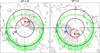 |
Fig. 1 The data coverage of THU2 data in geomagnetic latitude/magnetic local time coordinates. The red circle is the data coverage (extent of pierce points) of GPS data at a cutoff elevation of 30° by assuming pierce points at 350 km altitude. The left panel shows the data coverage at 15:00 UT when THU2 is located around magnetic noon, while the right panel shows for 3:00 UT when THU2 is located around magnetic midnight. The green shaded area is the auroral oval derived from the Feldstein model for Q = 3. |
The data from THU2 are downloaded from the IGS website (ftp://garner.ucsd.edu/pub/rinex), and the data are in RINEX format at 30 s temporal resolution. Only GPS data are used in this study. The GPS TEC data can be calculated from the carrier phase observations at L1 and L2 frequencies using the following formula:
![Mathematical equation: $$ {\mathrm{TEC}}_{\mathrm{\Phi }}=9.52\times \left[\left({\mathrm{\Phi }}_1-{\mathrm{\Phi }}_2\right)-{B}_{{rs}}-\Delta N\right] $$](/articles/swsc/full_html/2022/01/swsc210081/swsc210081-eq1.gif) (1)TECΦ is the slant TEC in a unit of TECU (1 TECU = 1× 10¹⁶ el·m−2), and Φ1 and Φ2 are the carrier phase observations at L1 and L2 frequencies. Brs are the instrumental biases (differential code biases) of the GPS satellites and receiver, and ∆N is the phase ambiguity. Brs are relatively stable over several days, and the phase ambiguity is constant over one continuous tracking arc (i.e., without cycle slips). From TEC, we can calculate the rate of change of TEC (ROT) which is the time derivative of TEC:
(1)TECΦ is the slant TEC in a unit of TECU (1 TECU = 1× 10¹⁶ el·m−2), and Φ1 and Φ2 are the carrier phase observations at L1 and L2 frequencies. Brs are the instrumental biases (differential code biases) of the GPS satellites and receiver, and ∆N is the phase ambiguity. Brs are relatively stable over several days, and the phase ambiguity is constant over one continuous tracking arc (i.e., without cycle slips). From TEC, we can calculate the rate of change of TEC (ROT) which is the time derivative of TEC:
 (2)where δt = 30 s, since we use the 30-s resolution RINEX data. Note that we use slant TEC to be consistent with (Pi et al., 1997). In this way, the instrumental biases and phase ambiguity are canceled out. We remove ROT with absolute values larger than 10 TECU/min to account for possible cycle slips. In addition, the ROT is smoothed using a median filter of the consecutive three data points to further remove the possible impact of small cycle clips.
When calculating ROTI, we use a similar method as Pi et al. (1997), i.e., the standard deviation of ROT in a running window of 5 min:
 (3)and
  is the mean of ROT(ti):
 (4)where ∆t = 300 s, i.e., 5 min.
We also use solar irradiance parameters and geomagnetic indices to characterize the space environment. The F10.7 index that measures the total emission at the wavelength of 10.7 cm of the solar disk is widely used to represent solar activity (e.g., Tapping, 2013). For modeling the ionosphere, the F10.7 index is often used (Bilitza et al., 2011). However, recent studies suggest that F10.7P “is recommended as a better solar proxy for common use in that it retains the advantages of F10.7 of a long-term record and good availability”. F10.7P is defined as (F10.7 + F10.7_81)/2, and F10.7_81 is the average of the F10.7 solar flux index in a running window of 81 days (3 solar rotations) (Rentz & Lühr, 2008; Xiong et al., 2010a). In addition, the sunspot number is also presented in the present study.
For the geomagnetic indices, we choose to use the Dst (Disturbance Storm Time) index. It is an hourly geomagnetic index that measures the intensity of the globally symmetrical equatorial electrojet (the “ring current”) and is derived from four magnetic observatories at low latitudes. The variations of Dst provide a quantitative measure of the level of geomagnetic disturbances that can be correlated with other solar and geophysical parameters. The Dst index can also be used to identify various phases of a geomagnetic storm. The original Dst index can be downloaded from the World Data Center for Geomagnetism, Kyoto (http://wdc.kugi.kyoto-u.ac.jp/dstdir/). For the present study, we use the daily averaged Dst index from the NASA CDAWeb (https://cdaweb.gsfc.nasa.gov/index.html/). In order to present the upstream interplanetary magnetic field (IMF), we use the daily average of the total magnetic field (Bt) from the OMNI dataset (King & Papitashvili, 2005).
3 Results
3.1 Typical observations
The GPS data used in this study are collected during two solar cycles, i.e., it contains completely different states of the polar cap ionosphere driven by different forcing in terms of solar irradiance, solar wind conditions, and the strength and orientations of IMF, etc. In order to show the nominal ionospheric conditions during different phases of solar activity, we present GPS data during 9 days near solar maximum in 2001 and solar minimum in 2020. The data are selected during the geomagnetic quiet condition (daily averaged Kp < 3) to isolate the impact of geomagnetic storms. We also choose the same season (winter) to avoid the control of seasonal variations. Figure 2 presents GPS vertical TEC and ROTI from THU2 in 2001 and 2020 from all available GPS satellites. To calculate the absolute GPS TEC, the instrumental biases of the GPS satellites and receiver should be removed (see Eq. (1)). For this purpose, we extracted the information on instrumental biases from the Center for Orbit Determination in Europe (CODE) (ftp://ftp.aiub.unibe.ch). The instrumental biases from both GPS receivers and satellites are removed from the TEC data in 2020, and thus they are correctly calibrated. However, the instrumental bias information for the THU2 receiver was not available in 2001 from CODE, and we use the least-squares method to estimate the instrumental biases of the GPS receiver (Bishop et al., 1995). The vertical TEC is converted using a single layer mapping function by assuming pierce points at 350 km altitude (see, e.g., Mannucci et al., 1998).
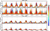 |
Fig. 2 Examples of vertical TEC and ROTI during different solar activities. (a–b) TEC and ROTI from December 3 to 12 near solar maximum in 2001. Different colors represent different satellites according to the PRN number in the color bar. (c–d) TEC and ROTI during 9 days near the solar minimum in 2020. |
Figure 2 clearly presents different states of the polar cap ionosphere between two years. In 2001, there were prominent TEC increases around noon and afternoon (increase from 5 TECU before sunrise to 50 TECU in early afternoon, i.e., TEC increase = ~45 TECU) every day. This is due to the diurnal variations of TEC, where the solar EUV ionization near local noon is the strongest. In 2020, the diurnal TEC increases were much weaker (TEC increase = 5–8 TECU). The ranges of ROTI were also quite different for different years, i.e., ROTI only reached up to ~2 TECU/min in 2020, while the value of 4 TECU/min was very common in 2001. This can be explained by a higher background density and strong forcing by auroral dynamics and flow channels during solar maximum in 2001. Besides the difference in the magnitude of the diurnal variations, the trend of these variations was quite similar, i.e., the TEC and ROTI all peaked around local noon (15–16 UT) with only sporadic increases at other local times.
3.2 Climatology
As shown in the previous sections, the GPS data contains two solar cycles with variable and sometimes distinctive ionospheric conditions. In this study, we will focus on the long-term climatology scale and not focus on timescales smaller than a month. To show the long-term variations, we arrange the ROTI data into bins of UT and month (1 h in UT for every month). The mean value in each bin from January 1999 to December 2021 is shown in Figure 3a. Data from two months were missing in the dataset (August in 2000 and April in 2019). Figure 3b shows the F10.7P index (black) and sunspot number (red). The F10.7P index and sunspot number show a similar trend in the solar cycle. Compared to the sunspot number, the F10.7P index is more commonly used in ionospheric modeling (Xiong et al., 2010b; Liu et al., 2011).
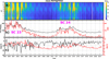 |
Fig. 3 (a) The averaged ROTI in bins of 1 h in UT and 1 month. (b) The F10.7P index (black) and monthly averaged sunspot number (red). (c) The monthly averaged Dst index (black) and the total interplanetary magnetic field (red). |
For the long-term variations, ROTI varied clearly with the solar activity, i.e., during solar maximums (1999–2003 and 2013–2015), the ROTI values were significantly bigger. Figure 3b shows that the high sunspot number (red) and high F10.7P index (black) matched with high values of ROTI. This implies that the most severe space conditions mostly occur during solar maximums. In addition to the solar cycle dependence, Figure 3a shows clear seasonal variations in the TEC irregularities. The enhanced ROTI values tended to occur during the winter period (October–February) and showed a minimum near June. Also, there were small minima near December in the middle of the enhanced wintertime ROTI, which is in line with previous studies (Prikryl et al., 2015; Meziane et al., 2020b). These features are called the annual variations (wintertime enhancement) and semi-annual variation (local minimum around December), and they are similar to the statistics of GPS phase scintillation from Ny-Ålesund at a slightly lower magnetic latitude (Jin et al., 2018). The ROTI data in Figure 3a also show a clear diurnal variation, i.e., ROTI is intensified around 15 UT (close to magnetic noon), and it remains at high values until 24 UT during solar maximum. During solar minimum, ROTI only shows a peak around 15 UT from equinoxes to summer, while the peak shifts to the afternoon and nightside sector from November to February. This feature is also consistent with the observation in the Canadian sector (Prikryl et al., 2015; Meziane et al., 2021). THU2 is a polar cap station (~83.5° MLAT, cf. Fig. 1). Around magnetic noon, the southern part of the data coverage is closer to the plasma entry region, i.e., the cusp location (~75° MLAT). Therefore, the plasma that enters the polar cap can be observed at Thule without obvious decay in density (Weber et al., 1986). During solar maximum, the transport of plasma in the form of a tongue of ionization/polar cap patches is the most prominent (Basu et al., 1985; Foster et al., 2005). Due to the relatively high latitude of the Thule station, the nominal nightside aurora is not expected to affect the observed ROTI.
Figure 3c shows the Dst index and IMF strength (Bt). The Dst index is commonly used to measure the intensity of geomagnetic storms (see e.g., Borovsky & Shprits, 2017 for the history and limitations of the Dst index). During geomagnetic storms, the status and variability of the ionosphere can be greatly affected (Buonsanto, 1999). During the peak of solar cycle 23 (2001–2003), there were a few severe geomagnetic storms (Dst was below −200 nT). Even the monthly averaged Dst index reached as low as −50 nT in 2002. The high-latitude ionosphere is directly coupled to the solar wind and IMF. The high-latitude convection patterns and the plasma transport are greatly modulated by the strength and orientation of the IMF. The IMF does not simply follow the solar cycle. Strong IMF is generally associated with the Coronal Mass Ejection (CME) and CIR. However, the statistical distribution of CMEs and CIRs are different with respect to the phases of a solar cycle (e.g., Tsurutani et al., 2006). Therefore, the IMF strength displays different variations in comparison to the sunspot number (solar cycle). Consequently, it is not redundant to include the IMF in describing the variability of the polar ionosphere.
3.3 EOF decomposition
Next, we describe how to decompose the climatological variations of ROTI into several main components. The empirical orthogonal function (EOF) method has been widely used to analyze the spatial and temporal variations of the atmosphere and ocean (Lorenz, 1956). It has been used in developing empirical models of the ionosphere (Dvinskikh & Naidenova, 1991). For example, the EOF analysis model has been successfully used to develop the global models of hmF2, foF2, and TEC maps (Zhang et al., 2009; A et al., 2011, 2012). Using the EOF method, the interested dataset can be effectively decomposed into a series of orthogonal base functions with corresponding EOF coefficients. These base functions are directly calculated from the original dataset, and they can reflect the inherent features of the original data. In addition, the advantage is that the EOF method converges very quickly, and only the first few EOFs can reflect the majority of the total data variability.
We use the climatological data of ROTI from 2000 to 2020 to develop the EOF model, while the data in 1999 and 2021 are only used for validation purposes. The climatology of ROTI is expressed by a 2-D matrix in UT and month (24 × 252) (cf. Fig. 3a). As shown in the previous section, ROTI shows solar cycle, seasonal and diurnal variations. The final model should also reflect temporal variations in these timescales. Using the EOF method, ROTI can be decomposed into the product of a series of orthogonal base functions (Ei) and the corresponding coefficients (Ai):
 (5)
(5)
Table 1 presents the percentage of total ROTI variability captured by the first four EOFs. Clearly, the first order EOF contributes to the majority (96.25%) of the total ROTI variability. The EOF converges very quickly, and the first four order EOFs contribute to 99.49% of the total variability. We, therefore, use the first four EOFs to build the climatological model of ROTI in the following.
The percentage of data variability captured by the first four Empirical Orthogonal Functions (EOFs)
The first four EOF functions and coefficients are presented in Figure 4, where the EOF base functions are shown on the left, and the corresponding coefficients are shown on the right. In addition, we also plot the mean ROTI in terms of diurnal variations in the top left panel of Figure 4. The mean ROTI represents the averaged behavior over all solar activity and seasons. It shows a minimum value at 6 UT, and it increases quickly from 12 UT to reach a peak at 15.5 UT (close to magnetic noon). The first base function E1 is similar to the averaged diurnal variations of ROTI and it shows the same trend as the averaged ROTI. The first coefficient A1 shows a similar trend as the mean ROTI over all UT. It reflects the solar activity and seasonal variations of the ROTI activity. The first EOF coefficient A1 was the highest during solar maximum (2000–2003 and 2012–2015), and it was the lowest during solar minimum. In addition, the seasonal variations were also very clear, i.e., A1 was the highest near December solstices. This behavior is similar to the seasonal variations of ROTI and GPS scintillations at high latitudes (e.g., Prikryl et al., 2015; Jin et al., 2018; Meziane et al., 2020b).
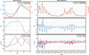 |
Fig. 4 The decomposed base functions (left column) and the associated coefficients (right column). The mean of ROTI data over all months is also presented in orange in the top left panel. The mean ROTI over all hours is plotted as an orange curve in the top right panel. |
The second base function E2 can be regarded as deviations from the averaged diurnal variations of ROTI and the first base function E1. The second EOF coefficient A2 represents the semi-annual variation, and it peaks around equinoxes. This behavior reflects typical characteristics of the high-latitude plasma irregularities, i.e., there is a small decrease in the amplitude of irregularities near December solstices. This is due to the decrease of the background electron density because of the low photo-ionization rate during the deep polar night. To explain the deviation of the second EOF base function from the averaged diurnal variation of ROTI, we show in Figure 5 the averaged ROTI in summer (May, June, and July) and winter (November, December, and January) months. Clearly, the mean ROTI is different between summer and winter, i.e., ROTI was higher, and it peaked at a later time (19.5 UT, evening side) in winter. This effect can be explained by the impact of solar illumination (Kelley et al., 1982; Jin et al., 2018). The sunlight can ionize the E region ionosphere and enhance the E region conductivity and the conducting E region can short circuit the F region irregularities by plasma diffusion (Vickrey & Kelley, 1982; Ivarsen et al., 2019). Therefore, the mean ROTI is lower in summer, and the wintertime ROTI peaks at later local time when the solar illumination is weaker. In addition, the solar insolation during summer can create new ionization and smooth the existing horizontal gradients in the whole polar cap. Consequently, there is a minimum in the observations of polar cap patches (or tongue of ionization) in the polar ionosphere during summer (Wood & Pryse, 2010; Spicher et al., 2017; Jin & Xiong, 2020). This can also explain the lower ROTI values in summer. Therefore, the second EOF base function presents the deviation of the wintertime ROTI from the averaged diurnal variations of ROTI. ROTI peaks at later local time, and this deviation is most prominent during December solstices (winter).
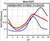 |
Fig. 5 The mean of ROTI data over all winter (November, December, and January) in black and summer (May, June, and July) months in blue. The mean ROTI over all seasons is also presented as a thick red line. |
The third and fourth EOFs only contribute 1% of the total ROTI variability, and the corresponding coefficients show some seasonal variations. However, it is difficult to explain the related sources/mechanisms for the two minor components.
Next, we fit the EOF coefficients using the solar flux (F10.7P index, sunspot number), solar wind conditions (solar wind speed, dynamic pressure, IMF, and Interplanetary Electric Field (IEF)), geomagnetic indices (Kp index, Dst index, Ap index, AE indices, and Polar Cap index). These geophysical parameters were obtained from the NASA CDAWeb. The high-latitude ionosphere is directly coupled to the solar wind and magnetosphere. We also calculate the correlation with the solar wind-magnetosphere coupling function as  , where θc is the clock angle of IMF, and V is the solar wind speed (Newell et al., 2007). The selected parameters and their correlation with the first four EOF coefficients are presented in Table 2. The correlation coefficients are obtained by correlating each EOF coefficient with the monthly averaged geophysical parameters. In Table 2, for the first EOF coefficient, we also highlight the three highest correlations (except the sunspot number) that reflect the main contribution. The first EOF coefficient is mainly driven by the F10.7P index, total IMF strength (Bt), and Dst index. Both F10.7P and the sunspot number can reflect solar irradiance. Due to the close relation and high correlation coefficient (0.98) between F10.7P and sunspot number (cf. Fig. 3b), we only use F10.7P as it gives a higher correlation coefficient with A1 (0.86 for F10.7P versus 0.81 for the sunspot number). The other two parameters are chosen to reflect the control of IMF and geomagnetic storms. Note that there are many geomagnetic indices, such as Dst, Kp, Ap, and AE indices, to characterize geomagnetic storms and substorms (see e.g., Borovsky & Shprits, 2017). However, we choose to use the Dst index as it gives a higher correlation coefficient, as shown in Table 2. Though the three selected geophysical parameters reflect three different classes of drivers, i.e., solar irradiance (F10.7P), IMF (Bt), and geomagnetic storm (Dst), there is also a correlation between them. The correlation coefficient for F10.7P versus the Dst index is −0.48, and it is 0.76 for F10.7P versus Bt. However, as the Sun is the dominant driver of the near-Earth space environment, the inter-connection through complex processes and unavoidable correlation between different geophysical parameters, especially on the long time scales, are not uncommon. Unlike the Bayesian framework (Meziane et al., 2021), the fits of the EOF coefficients do not require the fitting variables to be independent. Therefore, we choose to use the F10.7P index, total IMF strength (Bt), and Dst index to fit the EOF coefficients. The correlation coefficients for the other EOF coefficients are much lower. This indicates that it is more difficult to find the main sources of the other EOFs.
Correlation coefficients of the commonly used solar and geomagnetic indices with the first 4 EOF coefficients.
The procedure to fit the EOF coefficients is explained as follows:
 (6)
(6)
 (7)
(7)
![Mathematical equation: $$ {\mathbf{B}}_{i2}(m)=\left[{\mathbf{C}}_{i2}+{\mathbf{D}}_{i2}\times {P}_1(m)+{\mathbf{E}}_{i2}\times {P}_2(m)+{\mathbf{F}}_{i2}\times {P}_3(m)\enspace \right]\mathrm{cos}(2{\pi m}/12)+\left[{\mathbf{G}}_{i2}+{\mathbf{H}}_{i2}\times {P}_1(m)+{\mathbf{I}}_{i2}\times {P}_2(m)+{\mathbf{J}}_{i2}\times {P}_3(m)\enspace \right]\mathrm{sin}(2{\pi m}/12) $$](/articles/swsc/full_html/2022/01/swsc210081/swsc210081-eq10.gif) (8)
(8)
![Mathematical equation: $$ {\mathbf{B}}_{i3}(m)=\left[{\mathbf{C}}_{i3}+{\mathbf{D}}_{i3}\times {P}_1(m)+{\mathbf{E}}_{i3}\times {P}_2(m)+{\mathbf{F}}_{i3}\times {P}_3(m)\enspace \right]\mathrm{cos}(4{\pi m}/12)+\left[{\mathbf{G}}_{i3}+{\mathbf{H}}_{i3}\times {P}_1(m)+{\mathbf{I}}_{i3}\times {P}_2(m)+{\mathbf{J}}_{i3}\times {P}_3(m)\enspace \right]\mathrm{sin}(4{\pi m}/12) $$](/articles/swsc/full_html/2022/01/swsc210081/swsc210081-eq11.gif) (9)where Ai(m) is the ith EOF coefficient, and it is expressed by three components, Bi1, Bi2, Bi3, which represent the solar cycle, annual and semi-annual variations in the EOF coefficients, respectively. P1, P2 and P3 are the three selected geophysical parameters, namely the F10.7P index, IMF strength Bt and Dst index. The constants C, D, E, F, G, H, I, and J can be obtained using the linear regression method. The EOF coefficients and the fitted ones are presented in Figure 6. The fits using linear regressions agree with the EOF coefficients very well, with only small discrepancies during solar maximums of solar cycles 23 and 24.
(9)where Ai(m) is the ith EOF coefficient, and it is expressed by three components, Bi1, Bi2, Bi3, which represent the solar cycle, annual and semi-annual variations in the EOF coefficients, respectively. P1, P2 and P3 are the three selected geophysical parameters, namely the F10.7P index, IMF strength Bt and Dst index. The constants C, D, E, F, G, H, I, and J can be obtained using the linear regression method. The EOF coefficients and the fitted ones are presented in Figure 6. The fits using linear regressions agree with the EOF coefficients very well, with only small discrepancies during solar maximums of solar cycles 23 and 24.
 |
Fig. 6 The EOF coefficients and the fitted coefficients using three selected parameters (see text for more details). |
3.4 Data-model comparison
To perform a self-validation of the EOF model, its results were directly compared with the experimental data. Figures 7 and 8 show such comparisons of the ROTI data and the model results. Figure 7b is obtained from the first four EOF components calculated using equation (5), where the EOF base functions and EOF coefficients are directly decomposed from the ROTI data. Figure 7b shows that the first four EOF components can well represent the climatology of ROTI from the GPS data, as shown in Figure 7a, from both the long-term variations (solar cycle, seasonal) and short-term ones (diurnal variations). This confirms the rapid convergence of the EOF method such that the majority (99.49% in Table 1) of the ROTI climatology can be captured by the first four terms, as shown in Section 3.3. Figure 7c is obtained from the EOF model, where the three geophysical parameters (F10.7P, Bt and Dst) are used as input to calculate the EOF coefficients. The results from the EOF model can reflect the ROTI climatology, except Figure 7c is smoother than the ROTI data in Figure 7a. This is often the case for the climatological model, where the input parameters are averaged. However, the actual data represents the real ionospheric system, which contains variations, from smoothly and slowly varying climatological scale to rapid variations during storms.
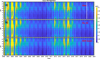 |
Fig. 7 (a) The climatology of ROTI from the Thule station; (b) the reconstructed ROTI climatology using equation (5); (c) the reconstructed ROTI climatology using the EOF model using the geophysical parameters as input. |
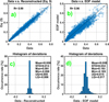 |
Fig. 8 The comparison of (a) reconstructed ROTI climatology using equation (5) and (b) EOF model versus the GPS ROTI data. The histogram of the bias (Data – Model) using equation (5) (c) and EOF model (d) in a bin step of 0.02 TECU/min. UQ = upper quartile; LQ = lower quartile. |
Figures 8a and 8b show the scatter plots of ROTI data versus the reconstructed ROTI using equation (5) and EOF model, respectively. The correlation coefficients are very high for both cases, i.e., 0.99 for that based on equation (5) and 0.96 for the EOF model using geophysical parameters. The correlation between data and the EOF model is slightly lower than that using equation (5). This should be related to the imperfect fit of the EOF coefficients in the EOF model, while equation (5) uses the EOF coefficients directly extracted from the data. To assess the performance of the model reconstruction, Figures 8c and 8d present the distribution of the bias between data and model in terms of the differences between modeled and experimental ROTI. The statistics of the differences such as the mean, standard deviation (STD), max, min, and upper (UQ), and lower quartiles (LQ) are also shown. For both cases, the mean is almost zero, which indicates that the model is not biased. This indicates that there is very little systematical underestimation or overestimation from the model. However, Figure 8d shows that there are slightly more occurrences of negative deviations for absolute deviations of less than 0.1 TECU/min. The STD of the deviations of the EOF model is 0.03 TECU/min, which is not significant. This suggests that the developed EOF model can well reflect the climatology of ROTI activity over the polar cap station at Thule, Greenland.
We also evaluate the performance of the model by comparing the model output with the experimental data in 1999 and 2021. The ROTI data in 1999 and 2021 are not used to build the EOF model, and this makes the testing dataset independent for the model validation. The results are shown in Figure 9 in a similar format as Figure 8. The left panels are for 1999 (close to solar maximum), while the right panels are for 2021 (close to solar minimum). For both cases, the linear correlation coefficients give satisfactory results, while the EOF model tends to underestimate the actual ROTI values in both cases. The error is bigger for the high solar activity year in 1999, where the mean error is 0.07 TECU/min with an STD of 0.07 TECU/min. These errors are close to the noise level of 0.05 TECU/min. A close look at Figure 9a suggests that the modeled ROTI agrees well with the experimental data within the ROTI range of 0.5 TECU/min. This is also the range for the majority of ROTI. For values larger than 0.5 TECU/min, the model obviously underestimates the actual ROTI activity. The performance during the low solar activity year in 2021 is much better. The mean error is 0.03 TECU/min with an STD of 0.02 TECU/min. This good performance is probably related to the low ROTI activity when the solar activity is low. As shown in Figure 7, the EOF model gives a smoother ROTI climatology than the experimental data. As the input geophysical parameters are monthly averaged, the most disturbed conditions with extreme geophysical parameters may be hidden in these averages. On the other hand, the most disturbed ionosphere during storms may make a high contribution to the climatology in the experimental data. We note that the probabilistic model based on the Bayesian framework also tends to underestimate the actual phase fluctuations at high latitudes (Meziane et al., 2021).
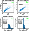 |
Fig. 9 (a–b) The comparison of reconstructed ROTI using the EOF model versus the experimental ROTI data. (c–d) The histogram of the bias (Data – Model) using a bin step of 0.02 TECU/min. UQ = upper quartile; LQ = lower quartile. |
3.5 Modeled ROTI in the Past and Future
An application of the EOF model is to reconstruct the historical ROTI activity over the past solar cycles. Since the EOF model only depends on three parameters, i.e., F10.7P, Bt, and Dst, the only requirement is that the three parameters should be available. While the first two geophysical parameters have been available for a long time (Dst from 1957 onwards, F10.7P from 1947 onwards), the IMF data can only be observed in-situ by artificial satellites in the solar wind. The IMF data have been incorporated into the “OMNI” dataset by the Space Physics Data Facility at NASA/Goddard Space Flight Center (Couzens & King, 1986). Though the IMF data can be obtained as early as 1963, the observations were relatively sparse at the beginning (Lockwood et al., 2017). We thus use the IMF data from 1965 when the solar wind data applicable in the present study are more continuous. For completeness, we also make predictions of the ROTI activity in the solar cycle 25. The Space Weather Prediction Center at National Oceanic and Atmospheric Administration (NOAA) predicts the monthly sunspot number and the monthly F10.7 of solar cycle 25. The predicted values are based on the consensus of the Solar Cycle 24 Prediction Panel (see https://www.swpc.noaa.gov/products/solar-cycle-progression). Figures 10a and 10b show the F10.7P index, sunspot number, Dst index, and IMF strength (Bt) from solar cycle 20 to the beginning of solar cycle 25. The predicted F10.7P and sunspot number from August 2021 are also shown. The F10.7P index and sunspot number show a clear periodicity of 11 years that defines the solar cycle. The IMF strength (Bt) also shows some variations with the solar cycle, with high values from the peak and the early declining phase of the solar cycles 21–24. For discussing geomagnetic storms and IMF during different phases of solar cycles, interested readers may refer to Tsurutani et al. (2006). One can also see that the solar cycle 24 is much weaker than solar cycle 23, which in turn is comparable to the previous three solar cycles, and these four solar cycles coincide within the so-called Modern Grand Maximum (1938–2000) (Lockwood et al., 2018). According to the prediction by NOAA, the solar cycle 25 will continue to be quiet (with F10.7P and sunspot numbers similar to or slightly weaker than solar cycle 24). Since there are no predictions of Bt and Dst for solar cycle 25, we use 5 nT for Bt and −9 nT for Dst for the whole solar cycle 25. These values are chosen to match the average values of Bt and Dst in solar cycle 24 (December 2008–December 2018). However, this choice may appear arbitrary as it cannot precisely reflect the variations of Bt and Dst during the phase of solar cycle 25.
 |
Fig. 10 (a) The monthly averaged F10.7P index (black), sunspot number (red). (b) The monthly averaged Dst index (black) and magnetic strength of IMF (red). (c) The reconstructed ROTI climatology in bins of 1 hour in UT by 1 month from 1965 to 2035. The predicted values of F10.7P and sunspot number are plotted from August 2021 to 2035. One month (July 2021) is intentionally omitted to separate observations and predictions. |
Figure 10c shows the reconstructed ROTI from the EOF model. The advantage of the EOF model is that it is now possible to quantitatively compare the space climate of ROTI irregularities across different periods even when the GPS data were not available. The solar cycle variations are clearly visible, where the solar cycles 21–22 had higher ROTI activity than solar cycle 23. This indicates that TEC irregularities were even more intense when the first GPS satellites were launched in the 1980s. Solar cycle 20 was during the modern space age when an increasing number of artificial satellites were launched into space. The ROTI irregularities in solar cycle 20 were weaker than in cycle 23 and stronger than in cycle 24. This indicates that the solar activity and ionospheric irregularities are entering a quiet period since the space era. As the predicted solar cycle 25 is similar to the activity of solar cycle 24, the ROTI activity should be similar to that during solar cycle 24. The peak phase of ROTI irregularities will be around the next solar maximum in 2025–2026, followed by a decrease in the ROTI activity. Because there are no predictions of Dst and Bt, the values used in the model may lead to overestimating the ROTI activity near solar minimum (2033–2035) and underestimation near solar maximum (2025–2026). With proper predictions of the solar activity and geophysical proxies, it is possible to predict the ROTI activity accordingly.
4 Discussion
This paper has developed a climatological model of ROTI over the polar cap station in Greenland based on the EOF method. The EOF method is suitable for developing the climatological model due to its quick convergence. Only the first few components can reflect the majority of the total data variability. The model is also quite simple to use, and it only depends on three geophysical parameters (F10.7P, Bt, and Dst). The model can well reflect the long-term variations (solar cycle, annual and semi-annual) and short-term variations (diurnal variations). The results of the model self-validation show that the model is accurate with a Pearson correlation coefficient of 0.96 and STD of 0.03 TECU/min. The validations against independent ROTI data in 1999 and 2021 also show satisfactory results. During the high solar activity year in 1999, the EOF model tended to underestimate the ROTI activity, with a mean bias of 0.07 TECU/min and STD of 0.07 TECU/min. During the low solar activity year in 2021, the EOF model also tends to underestimate the actual ROTI activity. However, the performance in 2021 appears better with a higher correlation (0.94 versus 0.90 in 1999), lower mean bias (0.03 TECU/min), and lower STD (0.02 TECU/min).
Only three geophysical parameters (F10.7P, Bt and Dst) are used in our model. This selection reflects different groups of geophysical drivers/sources (i.e., solar activity, IMF, and geomagnetic storms) of the high-latitude ionospheric variability and high correlation coefficients with the first EOF component. We note that different geophysical parameters have been used to develop space weather models in the literature. For example, to predict the high-latitude phase scintillation in the prediction time of 1 hour, McGranaghan et al. (2018) have selected 51 geophysical parameters. To avoid overfitting, their final model is driven by 25 parameters (including the current scintillation index, OVATION prime particle precipitation, AE index, Newell coupling function, dTEC, Kp index, Sym-H index, solar wind dynamic pressure, IMF Bz, and the location).Our model is quite simple compared to these variables, though different groups of geophysical drivers have already been represented in our model except particle precipitation. Despite the simplicity of our model, the validation with an independent dataset suggests that our model can already well represent the ROTI climatology (R=0.9, Mean = 0.07 TECU/min, STD = 0.07 TECU/min). Empirical models, which can represent the climatological ionosphere very well, often fail to represent the short timescales (or “weather-like”) variability. In other words, climatological models cannot satisfactorily represent the ionospheric environment on minute-to-minute, hour-to-hour, and day-to-day time scales. This feature is not due to the chosen method but because of the nature of ionospheric variability. Figure 11 presents the standard deviation of ROTI in bins of 1 hour by 1 month. The variance of ROTI shows clear solar cycle, annual, semi-annual and diurnal variations in the same manner as the mean ROTI. The standard deviation of ROTI is at the same level as the mean ROTI. This indicates that though the modeling of the climatological behaviors of ROTI can be very accurate, the variances around the mean ROTI are in the same order as the mean ROTI. This is due to the increased complexity of the space environment at high latitudes. The polar ionosphere is highly variable as it is affected by plasma transport in terms of tongue-of-ionization/polar cap patches, localized particle precipitation, flow channels, and various other geophysical processes. However, the climatological model such as the one in the present paper can still be useful as it can provide baselines for space weather monitoring and space segment operation.
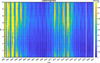 |
Fig. 11 The standard deviation (std) of ROTI in bins of 1 h by 1 month. It is clear that the variations of std (ROTI) also show solar cycle, seasonal, and diurnal variations in the same manner as the climatology of mean ROTI. |
On the other hand, one may argue that the deterministic model such as the present one and most of the available climatological models (e.g., WBMOD) cannot be used for operational purposes. The only way that seems to be adequate is to build a probabilistic model. For example, Meziane et al. (2021) developed a Bayesian inference-based empirical model for high-latitude scintillations. Once the prior probabilities are determined, the posterior probabilities can be directly deduced for an arbitrary set of predictors (Universal Time, F10.7 index, the maximum solar zenith angle, the solar wind ram pressure and speed, IMF By and Bz components, the SuperMAG auroral Electrojet (SME) index (similar to AE index)). The results are satisfactory on hourly averaged values of GPS phase and amplitude scintillation indices. However, it is not known what the magnitude of the standard deviations around the hourly averaged values is. In any case, the study suggests that the future space weather forecast products may consider probabilistic models for operational purposes. Our model is a regional model that calculates ionospheric irregularities in the central polar cap (Greenland). For example, we can estimate the GNSS carrier phase tracking errors in terms of ROTI calculated from the EOF model. Ionospheric irregularities and scintillations affect the delay-locked loop and phase-locked loop (PLL) of GNSS receivers. With a proper model of the receiver design, one can also estimate the tracking performance of the user receiver (Conker et al., 2003). This model can also be used for the mitigation of the scintillation effect caused by ionospheric irregularities. For example, Tiwari et al. (2011) used the WBMOD scintillation model to mitigate the scintillation effect at high latitudes. Strong scintillations can cause a loss of phase lock for PLL, resulting in no GNSS signal available. A PLL with a larger bandwidth (at the expense of extra phase noise) can avoid loss of lock due to the scintillation effect. Increasing the bandwidth during intense scintillations (predicted by models) allows one to receive a GNSS signal during scintillation conditions.
Another way to complement the climatological model is to construct the distribution function of ROTI. Figure 12 presents the occurrence rate of ROTI in bins of 0.02 TECU/min as blue bars. The red curve presents the fitted probability density function (PDF) of ROTI in the form of the lognormal distribution. The lognormal distribution is only dependent on two parameters, i.e., μ and σ, where μ is the mean of logarithmic values and σ is the standard deviation of logarithmic values. It is possible to make models of μ and σ using the EOF method. Once μ and σ are obtained, the associated PDF is defined. The advantage of the lognormal distribution is that the two parameters have their physical meanings (mean and standard deviation). From the PDF of ROTI, it is straightforward to calculate the occurrence rate of ROTI above certain values (e.g., extreme events) in the same manner as the occurrences of storms and substorms (Lockwood et al., 2018). This is a probabilistic forecast, i.e., to predict the probability and likelihood of space weather events above certain thresholds. The work to fit and model of the distribution functions will be left for future studies. Note that there exist other ways of fitting the ionospheric variability. For example, Meziane et al. (2020a) fitted the distribution of the GPS phase scintillation index (σφ) using 4 parameters (α, β, γ, δ), where the distribution function fα,β,γ,δ(x) can be simplified to several well-known distributions such as Gaussian (α = 2,  , and δ = μ), and Levy (α = 1/2, β = 1) distributions. However, the detailed discussions of the best distribution functions are beyond the scope of the present study.
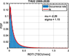 |
Fig. 12 The occurrence rate of ROTI during 2000–2020. The probability density function (PDF) is fitted with lognormal distribution by the red line. The fitted parameters are also displayed. |
5. Summary and conclusion
Using ROTI, we have presented the long-term climatology (over two solar cycles) of TEC irregularities from a polar cap station (Thule). The climatology reveals variability with different time scales, i.e., solar cycle, seasonal, and diurnal variations. These variations can be explained by different drivers/contributors. The solar activity (represented by the solar radiation index F10.7P) dominates in the longest time scale variations. The seasonal variations are controlled by the interplay of the energy input into the polar cap ionosphere and the solar illumination that damps the amplitude of ionospheric irregularities. The diurnal variations (with respect to local time) are controlled by the relative location of the station and the auroral oval. For example, enhanced ROTI values occur around 15–16 UT (close to magnetic noon) when the station is close to the nominal cusp, while the ROTI values are relatively low at night when Thule is far away from the nightside auroral zone. Furthermore, this kind of diurnal variation is clearly different between different seasons (cf. Fig. 5). During summer, ROTI peaks around 15.5 UT (close to magnetic noon), while it peaks around 19.5 UT (evening) in winter. This effect is again controlled by solar illumination.
The climatology is decomposed into a series of components using the EOF method. The first four EOFs reflect 99.49% of the total ROTI variability. The first EOF is the dominant component that contains 96.25% of the total variability. The first EOF base function reflects the diurnal variations of the mean ROTI. The first EOF coefficient represents mostly the solar activity dependence (solar cycle) and annual variations. The second EOF base function reflects the deviation from the mean diurnal variation, and the deviation is the most prominent during winter. The second EOF coefficient mainly represents seasonal variations in the semi-annual scales.
By fitting the EOF coefficients using only three geophysical proxies (namely, F10.7P, Bt, and Dst), we can effectively model the climatology of ROTI variations. The data-model comparisons show a satisfactory result with a Pearson correlation coefficient of 0.96. The validation using data outside the model training dataset reveals that the EOF model underestimates the actual ROTI. However, the error is within 0.1 TECU/min. Additionally, we modeled the ROTI during the Modern Grand Maximum dating back to 1965 and made predictions in solar cycle 25. In such a way, we can directly compare the climatic variations of ROTI across six solar cycles. The modeled results can reveal the averaged activity of TEC irregularities and indicate the severity of the space weather condition in the long term. Given the three needed proxies, this model is capable of making the long-term prediction of the future space weather climatology and reconstructing historical data.
This EOF model is relatively simple in use and easy to develop. This method is also useful for developing models for other irregularity indices that characterize ionospheric irregularities. Such applications may be useful in the GNSS amplitude and phase scintillation indices from ground-based GNSS scintillation receivers, as well as for other irregularity parameters measured using in-situ techniques from Low Earth Orbiting satellites such as Swarm (Jin et al., 2019). In addition, it is also possible to expand the 1-D model into a 2-D map of ROTI irregularities over the whole Arctic area.
Acknowledgments
This work is funded by ESA ITT “Forecasting Space Weather Impacts on Navigation Systems in the Arctic (Greenland Area)” Expro+, Activity No. 1000026374. This research is a part of the 4DSpace Strategic Research Initiative at the University of Oslo. YJ acknowledges funding from RCN grant 235655. WJM acknowledges funding from the European Research Council (ERC) under the European Union’s Horizon 2020 research and innovation program (ERC Consolidator Grant agreement No. 866357, POLAR-4DSpace). This research is a part of the 4DSpace Strategic Research Initiative at the University of Oslo. The GNSS RINEX data can be obtained through ftp://garner.ucsd.edu/pub/rinex/. The GPS instrumental biases can be downloaded from ftp://ftp.aiub.unibe.ch. The F10.7 index, Dst index, and IMF data can be obtained through https://omniweb.gsfc.nasa.gov/form/dx1.html. The editor thanks Anton Kashcheyev and an anonymous reviewer for their assistance in evaluating this paper.
References
- Aa E, Zhang D, Ridley AJ, Xiao Z, Hao Y. 2012. A global model: Empirical orthogonal function analysis of total electron content 1999–2009 data. J Geophys Res (Space Phys) 117(A3). https://doi.org/10.1029/2011JA017238. [Google Scholar]
- Aa E, Zhang DH, Xiao Z, Hao YQ, Ridley AJ, Moldwin M. 2011. Modeling ionospheric foF2 by using empirical orthogonal function analysis. Ann Geophys 29(8): 1501–1515. https://doi.org/10.5194/angeo-29-1501-2011. [CrossRef] [Google Scholar]
- Alfonsi L, Spogli L, De Franceschi G, Romano V, Aquino M, Dodson A, Mitchell CN. 2011. Bipolar climatology of GPS ionospheric scintillation at solar minimum. Radio Sci 46: Rs0d05. https://doi.org/10.1029/2010rs004571. [Google Scholar]
- Basu S, Basu S, Mackenzie E, Whitney HE. 1985. Morphology of phase and intensity scintillations in the auroral oval and polar-cap. Radio Sci 20(3): 347–356. https://doi.org/10.1029/RS020i003p00347. [CrossRef] [Google Scholar]
- Basu S, Groves KM, Basu S, Sultan PJ. 2002. Specification and forecasting of scintillations in communication/navigation links: Current status and future plans. J Atmos Sol Terr Phys 64(16): 1745–1754. https://doi.org/10.1016/s1364-6826(02)00124-4. [CrossRef] [Google Scholar]
- Basu S, Groves KM, Quinn JM, Doherty P. 1999. A comparison of TEC fluctuations and scintillations at Ascension Island. J Atmos Sol Terr Phys 61(16): 1219–1226. https://doi.org/10.1016/S1364-6826(99)00052-8. [CrossRef] [Google Scholar]
- Bilitza D, McKinnell L-A, Reinisch B, Fuller-Rowell T. 2011. The international reference ionosphere today and in the future. J Geod 85(12): 909–920. https://doi.org/10.1007/s00190-010-0427-x. [CrossRef] [Google Scholar]
- Bishop G, Mazzella A, Holland E. 1995. Using the lonosphere for BPS Measurement Error Control. In: Proceedings of the 8th International Technical Meeting of the Satellite Division of the Institute of Navigation (ION GPS 1995), Palm Springs, CA, September, pp. 1091–1100. https://www.ion.org/publications/abstract.cfm?articleID=2343. [Google Scholar]
- Borovsky JE, Shprits YY. 2017. Is the Dst index sufficient to define all geospace storms? J Geophys Res (Space Phys) 122(11): 11543–11547. https://doi.org/10.1002/2017JA024679. [Google Scholar]
- Buonsanto MJ. 1999. Ionospheric storms – a review. Space Sci Rev 88(3): 563–601. https://doi.org/10.1023/A:1005107532631. [CrossRef] [Google Scholar]
- Cherniak I, Krankowski A, Zakharenkova I. 2014. Observation of the ionospheric irregularities over the Northern Hemisphere: Methodology and service. Radio Sci 49(8): 653–662. https://doi.org/10.1002/2014RS005433. [CrossRef] [Google Scholar]
- Cherniak I, Krankowski A, Zakharenkova I. 2018. ROTI Maps: A new IGS ionospheric product characterizing the ionospheric irregularities occurrence. GPS Solut 22(3): 69. https://doi.org/10.1007/s10291-018-0730-1. [CrossRef] [Google Scholar]
- Conker RS, El-Arini MB, Hegarty CJ, Hsiao T. 2003. Modeling the effects of ionospheric scintillation on GPS/Satellite-Based Augmentation System availability. Radio Science 38(1): 1001. https://doi.org/10.1029/2000RS002604. [Google Scholar]
- Couzens DA, King JH. 1986. Interplanetary medium data book. Supplement 3: 1977-1985 (Rep. NSSDC/WDC-A/R&S, 86-04). NASA, Greenbelt, MD. [Google Scholar]
- De Franceschi G, Spogli L, Alfonsi L, Romano V, Cesaroni C, Hunstad I. 2019. The ionospheric irregularities climatology over Svalbard from solar cycle 23. Sci Rep 9: 9232. https://doi.org/10.1038/s41598-019-44829-5. [CrossRef] [Google Scholar]
- Dvinskikh NI, Naidenova NI. 1991. An adaptable regional empirical ionospheric model. Adv Space Res 11: 7. https://doi.org/10.1016/0273-1177(91)90312-8. [CrossRef] [Google Scholar]
- Emmert JT, Richmond AD, Drob DP. 2010. A computationally compact representation of magnetic-apex and quasi-dipole coordinates with smooth base vectors. J Geophys Res (Space Phys) 115: A8. https://doi.org/10.1029/2010ja015326. [Google Scholar]
- Forte B. 2005. Optimum detrending of raw GPS data for scintillation measurements at auroral latitudes. J Atmos Sol Terr Phys 67(12): 1100–1109. https://doi.org/10.1016/j.jastp.2005.01.011. [CrossRef] [Google Scholar]
- Foster JC, Coster AJ, Erickson PJ, Holt JM, Lind FD, et al. 2005. Multiradar observations of the polar tongue of ionization. J Geophys Res (Space Phys) 110: A9. https://doi.org/10.1029/2004ja010928. [Google Scholar]
- Holzworth RH, Meng CI. 1975. Mathematical representation of auroral oval. Geophys Res Lett 2(9): 377–380. https://doi.org/10.1029/GL002i009p00377. [CrossRef] [Google Scholar]
- Ivarsen MF, Jin Y, Spicher A, Clausen LB. 2019. Direct evidence for the dissipation of small-scale ionospheric plasma structures by a conductive E region. J Geophys Res (Space Phys) 124(4): 2935–2942. https://doi.org/10.1029/2019JA026500. [Google Scholar]
- Jacobsen KS. 2014. The impact of different sampling rates and calculation time intervals on ROTI values. J Space Weather Space Clim 4: A33. https://doi.org/10.1051/swsc/2014031. [CrossRef] [EDP Sciences] [Google Scholar]
- Jacobsen KS, Dahnn M. 2014. Statistics of ionospheric disturbances and their correlation with GNSS positioning errors at high latitudes. J Space Weather Space Clim 4: A27. https://doi.org/10.1051/swsc/2014024. [CrossRef] [EDP Sciences] [Google Scholar]
- Jakowski N, Beniguel Y, De Franceschi G, Pajares MH, Jacobsen KS, et al. 2012. Monitoring, tracking and forecasting ionospheric perturbations using GNSS techniques. J Space Weather Space Clim 2: 14. https://doi.org/10.1051/swsc/2012022. [Google Scholar]
- Jin Y, Xiong C. 2020. Interhemispheric Asymmetry of Large-Scale Electron Density Gradients in the Polar Cap Ionosphere: UT and Seasonal Variations. J Geophys Res (Space Phys) 125(2): e2019JA027601. https://doi.org/10.1029/2019ja027601. [Google Scholar]
- Jin YQ, Miloch WJ, Moen JI, Clausen LBN. 2018. Solar cycle and seasonal variations of the GPS phase scintillation at high latitudes. J Space Weather Space Clim 8: A48. https://doi.org/10.1051/swsc/2018034. [CrossRef] [EDP Sciences] [Google Scholar]
- Jin YQ, Moen JI, Miloch WJ. 2014. GPS scintillation effects associated with polar cap patches and substorm auroral activity: direct comparison. J Space Weather Space Clim 4: A23. https://doi.org/10.1051/swsc/2014019. [CrossRef] [EDP Sciences] [Google Scholar]
- Jin YQ, Moen JI, Miloch WJ, Clausen LBN, Oksavik K. 2016. Statistical study of the GNSS phase scintillation associated with two types of auroral blobs. J Geophys Res (Space Phys) 121(5): 4679–4697. https://doi.org/10.1002/2016ja022613. [CrossRef] [Google Scholar]
- Jin YQ, Moen JI, Oksavik K, Spicher A, Clausen LBN, Miloch WJ. 2017. GPS scintillations associated with cusp dynamics and polar cap patches. J Space Weather Space Clim 7: A23. https://doi.org/10.1051/swsc/2017022. [CrossRef] [EDP Sciences] [Google Scholar]
- Jin YQ, Spicher A, Xiong C, Clausen LBN, Kervalishvili G, Stolle C, Miloch WJ. 2019. Ionospheric plasma irregularities characterized by the swarm satellites: statistics at high latitudes. J Geophys Res (Space Phys) 124(2): 1262–1282. https://doi.org/10.1029/2018ja026063. [CrossRef] [Google Scholar]
- Kelley MC, Vickrey JF, Carlson CW, Torbert R. 1982. On the origin and spatial extent of high-latitude F-region irregularities. J Geophys Res (Space Phys) 87(Na6): 4469–4475. https://doi.org/10.1029/JA087iA06p04469. [CrossRef] [Google Scholar]
- King JH, Papitashvili NE. 2005. Solar wind spatial scales in and comparisons of hourly Wind and ACE plasma and magnetic field data. J Geophys Res (Space Phys) 110: A2. https://doi.org/10.1029/2004ja010649. [Google Scholar]
- Kintner PM, Ledvina BM, De Paula ER. 2007. GPS and ionospheric scintillations. Space Weather 5: S09003. https://doi.org/10.1029/2006sw000260. [Google Scholar]
- Kotulak K, Zakharenkova I, Krankowski A, Cherniak I, Wang N, Fron A. 2020. Climatology characteristics of ionospheric irregularities described with GNSS ROTI. Remote Sens 12(16): 2634. https://doi.org/10.3390/rs12162634. [CrossRef] [Google Scholar]
- Li GZ, Ning BQ, Ren ZP, Hu LH. 2010. Statistics of GPS ionospheric scintillation and irregularities over polar regions at solar minimum. GPS Solut 14(4): 331–341. https://doi.org/10.1007/s10291-009-0156-x. [CrossRef] [Google Scholar]
- Liu L, Wan W, Chen Y, Le H. 2011. Solar activity effects of the ionosphere: A brief review. Chin Sci Bull 56(12): 1202–1211. https://doi.org/10.1007/s11434-010-4226-9. [CrossRef] [Google Scholar]
- Lockwood M, Owens MJ, Barnard LA, Scott CJ, Watt CE. 2017. Space climate and space weather over the past 400 years: 1. The power input to the magnetosphere. J Space Weather Space Clim 7: A19. https://doi.org/10.1051/swsc/2017019. [Google Scholar]
- Lockwood M, Owens MJ, Barnard LA, Scott CJ, Watt CE, Bentley S. 2018. Space climate and space weather over the past 400 years: 2. Proxy indicators of geomagnetic storm and substorm occurrence. J Space Weather Space Clim 8: A12. https://doi.org/10.1051/swsc/2017048. [CrossRef] [EDP Sciences] [Google Scholar]
- Lorenz EN. 1956. Empirical orthogonal functions and statistical weather prediction. Massachusetts Institute of Technology, Department of Meteorology, Cambridge. [Google Scholar]
- Mannucci AJ, Wilson BD, Yuan DN, Ho CH, Lindqwister UJ, Runge TF. 1998. A global mapping technique for GPS-derived ionospheric total electron content measurements. Radio Sci 33(3): 565–582. https://doi.org/10.1029/97rs02707. [CrossRef] [Google Scholar]
- McGranaghan RM, Mannucci AJ, Wilson B, Mattmann CA, Chadwick R. 2018. New capabilities for prediction of high-latitude ionospheric scintillation: A novel approach with machine learning. Space Weather 16(11): 1817–1846. https://doi.org/10.1029/2018SW002018. [Google Scholar]
- Meziane K, Kashcheyev A, Jayachandran PT, Hamza AM. 2020a. On the latitude-dependence of the GPS phase variation index in the polar region. In: 2020 IEEE International Conference on Wireless for Space and Extreme Environments (WiSEE), pp. 72–77. https://doi.org/10.1109/WiSEE44079.2020.9262655. [CrossRef] [Google Scholar]
- Meziane K, Kashcheyev A, Jayachandran PT, Hamza AM. 2021. A Bayesian inference-based empirical model for scintillation indices for high-latitude. Space Weather 19(6): e2020SW002710. https://doi.org/10.1029/2020SW002710. [CrossRef] [Google Scholar]
- Meziane K, Kashcheyev A, Patra S, Jayachandran PT, Hamza AM. 2020b. Solar cycle variations of GPS amplitude scintillation for the polar region. Space Weather 18(8): e2019SW002434. https://doi.org/10.1029/2019SW002434. [CrossRef] [Google Scholar]
- Moen J, Oksavik K, Alfonsi L, Daabakk Y, Romano V, Spogli L. 2013. Space weather challenges of the polar cap ionosphere. J Space Weather Space Clim 3: A8. https://doi.org/10.1051/swsc/2013025. [Google Scholar]
- Newell PT, Sotirelis T, Liou K, Meng CI, Rich FJ. 2007. A nearly universal solar wind-magnetosphere coupling function inferred from 10 magnetospheric state variables. J Geophys Res (Space Phys) 112: A1. https://doi.org/10.1029/2006ja012015. [Google Scholar]
- Pi X, Mannucci AJ, Lindqwister UJ, Ho CM. 1997. Monitoring of global ionospheric irregularities using the worldwide GPS network. Geophys Res Lett 24(18): 2283–2286. https://doi.org/10.1029/97gl02273. [CrossRef] [Google Scholar]
- Prikryl P, Jayachandran PT, Chadwick R, Kelly TD. 2015. Climatology of GPS phase scintillation at northern high latitudes for the period from 2008 to 2013. Ann Geophys 33(5): 531–545. https://doi.org/10.5194/angeo-33-531-2015. [CrossRef] [Google Scholar]
- Prikryl P, Jayachandran PT, Mushini SC, Chadwick R. 2011. Climatology of GPS phase scintillation and HF radar backscatter for the high-latitude ionosphere under solar minimum conditions. Ann Geophys 29(2): 377–392. https://doi.org/10.5194/angeo-29-377-2011. [CrossRef] [Google Scholar]
- Prikryl P, Jayachandran PT, Mushini SC, Richardson IG. 2012. Toward the probabilistic forecasting of high-latitude GPS phase scintillation. Space Weather 10: S08005. https://doi.org/10.1029/2012sw000800. [Google Scholar]
- Prikryl P, Sreeja V, Aquino M, Jayachandran PT. 2013. Probabilistic forecasting of ionospheric scintillation and GNSS receiver signal tracking performance at high latitudes. Ann Geophys 56(2). https://doi.org/10.4401/ag-6219. [Google Scholar]
- Priyadarshi S. 2015a. Ionospheric scintillation modeling for high- and mid-latitude using B-spline technique. Astrophys Space Sci 359(1): 12. https://doi.org/10.1007/s10509-015-2461-x. [CrossRef] [Google Scholar]
- Priyadarshi S. 2015b. A Review of Ionospheric Scintillation Models. Surveys in Geophysics 36(2): 295–324. https://doi.org/10.1007/s10712-015-9319-1. [CrossRef] [Google Scholar]
- Rentz S, Lühr H. 2008. Climatology of the cusp-related thermospheric mass density anomaly, as derived from CHAMP observations. Ann Geophys 26: 2807–2823. [CrossRef] [Google Scholar]
- Richmond AD. 1995. Ionospheric electrodynamics using magnetic apex coordinates. J Geomag Geoelec 47(2): 191–212. https://doi.org/10.5636/jgg.47.191. [CrossRef] [Google Scholar]
- Secan JA, Bussey RM, Fremouw EJ, Basu S. 1997. High-latitude upgrade to the wideband ionospheric scintillation model. Radio Sci 32(4): 1567–1574. https://doi.org/10.1029/97RS00453. [CrossRef] [Google Scholar]
- Semeter J, Mrak S, Hirsch M, Swoboda J, Akbari H, et al. 2017. GPS signal corruption by the discrete aurora: Precise measurements from the Mahali Experiment. Geophys Res Lett 44(19): 9539–9546. https://doi.org/10.1002/2017GL073570. [CrossRef] [Google Scholar]
- Spicher A, Clausen LBN, Miloch WJ, Lofstad V, Jin Y, Moen JI. 2017. Interhemispheric study of polar cap patch occurrence based on Swarm in situ data. J Geophys Res (Space Phys) 122(3): 3837–3851. https://doi.org/10.1002/2016ja023750. [CrossRef] [Google Scholar]
- Spogli L, Alfonsi L, De Franceschi G, Romano V, Aquino MHO, Dodson A. 2009. Climatology of GPS ionospheric scintillations over high and mid-latitude European regions. Ann Geophys 27(9): 3429–3437. https://doi.org/10.5194/angeo-27-3429-2009. [CrossRef] [Google Scholar]
- Tapping KF. 2013. The 10.7 cm solar radio flux (F10.7). Space Weather 11(7): 394–406. https://doi.org/10.1002/swe.20064. [CrossRef] [Google Scholar]
- Tiwari R, Skone S, Tiwari S, Strangeways HJ. 2011. WBMod assisted PLL GPS software receiver for mitigating scintillation affect in high latitude region. In: 2011 XXXth URSI General Assembly and Scientific Symposium, 2011, pp. 1–4. https://doi.opg/10.1109/URSIGASS.2011.6050861. [Google Scholar]
- Tsurutani BT, Gonzalez WD, Gonzalez ALC, Guarnieri FL, Gopalswamy N, et al. 2006. Corotating solar wind streams and recurrent geomagnetic activity: A review. J Geophys Res (Space Phys) 111: A7. https://doi.org/10.1029/2005ja011273. [Google Scholar]
- Van der Meeren C, Oksavik K, Lorentzen D, Moen JI, Romano V. 2014. GPS scintillation and irregularities at the front of an ionization tongue in the nightside polar ionosphere. J Geophys Res (Space Phys) 119(10): 8624–8636. https://doi.org/10.1002/2014ja020114. [CrossRef] [Google Scholar]
- Van Dierendonck AJ, Klobuchar J, Hua Q. 1993. Ionospheric scintillation monitoring using commercial single frequency C/A code receivers. Proceedings of the 6th International Technical Meeting of the Satellite Division of The Institute of Navigation (ION GPS 1993), Salt Lake City, UT, September 22–24, 1993, pp. 1333–1342. [Google Scholar]
- Vickrey JF, Kelley MC. 1982. The effects of a conducting E-layer on classical F-region cross-field plasma-diffusion. J Geophys Res (Space Phys) 87(Na6): 4461–4468. https://doi.org/10.1029/JA087iA06p04461. [CrossRef] [Google Scholar]
- Wang Y, Zhang Q-H, Jayachandran PT, Lockwood M, Zhang S-R, et al. 2016. A comparison between large-scale irregularities and scintillations in the polar ionosphere. Geophysical Research Letters 43(10): 4790–4798. https://doi.org/10.1002/2016GL069230. [CrossRef] [Google Scholar]
- Weber EJ, Klobuchar JA, Buchau J, Carlson HC, Livingston RC, et al. 1986. Polar cap-F layer patches – Structure and dynamics. J Geophys Res (Space Phys) 91(A11): 2121–2129. https://doi.org/10.1029/JA091iA11p12121. [Google Scholar]
- Wernik AW, Alfonsi L, Materassi M. 2007. Scintillation modeling using in situ data. Radio Sci 42(1): RS1002. https://doi.org/10.1029/2006RS003512. [Google Scholar]
- Wood AG, Pryse SE. 2010. Seasonal influence on polar cap patches in the high-latitude nightside ionosphere. J Geophys Res (Space Phys) 115. A7. https://doi.org/10.1029/2009ja014985. [Google Scholar]
- Xiong C, Park J, Luehr H, Stolle C, Ma SY. 2010a. Comparing plasma bubble occurrence rates at CHAMP and GRACE altitudes during high and low solar activity. Ann Geophys 28(9): 1647–1658. https://doi.org/10.5194/angeo-28-1647-2010. [CrossRef] [Google Scholar]
- Xiong C, Park J, Lühr H, Stolle C, Ma SY. 2010b. Comparing plasma bubble occurrence rates at CHAMP and GRACE altitudes during high and low solar activity. Ann Geophys 28(9): 1647–1658. https://doi.org/10.5194/angeo-28-1647-2010. [CrossRef] [Google Scholar]
- Yeh KC, Liu C-H. 1982. Radio wave scintillations in the ionosphere. Proc IEEE 70(4): 324–360. https://doi.org/10.1109/PROC.1982.12313. [CrossRef] [Google Scholar]
- Zhang ML, Liu C, Wan W, Liu L, Ning B. 2009. A global model of the ionospheric F2 peak height based on EOF analysis. Ann Geophys 27(8): 3203–3212. https://doi.org/10.5194/angeo-27-3203-2009. [CrossRef] [Google Scholar]
Cite this article as: Jin Y, Clausen LBN, Miloch WJ, Høeg P, Jarmołowski W, et al. 2022. Climatology and modeling of ionospheric irregularities over Greenland based on empirical orthogonal function method. J. Space Weather Space Clim. 12, 23. https://doi.org/10.1051/swsc/2022022.
All Tables
The percentage of data variability captured by the first four Empirical Orthogonal Functions (EOFs)
Correlation coefficients of the commonly used solar and geomagnetic indices with the first 4 EOF coefficients.
All Figures
|
Fig. 1 The data coverage of THU2 data in geomagnetic latitude/magnetic local time coordinates. The red circle is the data coverage (extent of pierce points) of GPS data at a cutoff elevation of 30° by assuming pierce points at 350 km altitude. The left panel shows the data coverage at 15:00 UT when THU2 is located around magnetic noon, while the right panel shows for 3:00 UT when THU2 is located around magnetic midnight. The green shaded area is the auroral oval derived from the Feldstein model for Q = 3. |
| In the text | |
|
Fig. 2 Examples of vertical TEC and ROTI during different solar activities. (a–b) TEC and ROTI from December 3 to 12 near solar maximum in 2001. Different colors represent different satellites according to the PRN number in the color bar. (c–d) TEC and ROTI during 9 days near the solar minimum in 2020. |
| In the text | |
|
Fig. 3 (a) The averaged ROTI in bins of 1 h in UT and 1 month. (b) The F10.7P index (black) and monthly averaged sunspot number (red). (c) The monthly averaged Dst index (black) and the total interplanetary magnetic field (red). |
| In the text | |
|
Fig. 4 The decomposed base functions (left column) and the associated coefficients (right column). The mean of ROTI data over all months is also presented in orange in the top left panel. The mean ROTI over all hours is plotted as an orange curve in the top right panel. |
| In the text | |
|
Fig. 5 The mean of ROTI data over all winter (November, December, and January) in black and summer (May, June, and July) months in blue. The mean ROTI over all seasons is also presented as a thick red line. |
| In the text | |
|
Fig. 6 The EOF coefficients and the fitted coefficients using three selected parameters (see text for more details). |
| In the text | |
|
Fig. 7 (a) The climatology of ROTI from the Thule station; (b) the reconstructed ROTI climatology using equation (5); (c) the reconstructed ROTI climatology using the EOF model using the geophysical parameters as input. |
| In the text | |
|
Fig. 8 The comparison of (a) reconstructed ROTI climatology using equation (5) and (b) EOF model versus the GPS ROTI data. The histogram of the bias (Data – Model) using equation (5) (c) and EOF model (d) in a bin step of 0.02 TECU/min. UQ = upper quartile; LQ = lower quartile. |
| In the text | |
|
Fig. 9 (a–b) The comparison of reconstructed ROTI using the EOF model versus the experimental ROTI data. (c–d) The histogram of the bias (Data – Model) using a bin step of 0.02 TECU/min. UQ = upper quartile; LQ = lower quartile. |
| In the text | |
|
Fig. 10 (a) The monthly averaged F10.7P index (black), sunspot number (red). (b) The monthly averaged Dst index (black) and magnetic strength of IMF (red). (c) The reconstructed ROTI climatology in bins of 1 hour in UT by 1 month from 1965 to 2035. The predicted values of F10.7P and sunspot number are plotted from August 2021 to 2035. One month (July 2021) is intentionally omitted to separate observations and predictions. |
| In the text | |
|
Fig. 11 The standard deviation (std) of ROTI in bins of 1 h by 1 month. It is clear that the variations of std (ROTI) also show solar cycle, seasonal, and diurnal variations in the same manner as the climatology of mean ROTI. |
| In the text | |
|
Fig. 12 The occurrence rate of ROTI during 2000–2020. The probability density function (PDF) is fitted with lognormal distribution by the red line. The fitted parameters are also displayed. |
| In the text | |
Current usage metrics show cumulative count of Article Views (full-text article views including HTML views, PDF and ePub downloads, according to the available data) and Abstracts Views on Vision4Press platform.
Data correspond to usage on the plateform after 2015. The current usage metrics is available 48-96 hours after online publication and is updated daily on week days.
Initial download of the metrics may take a while.