Dynamic modeling of the Earth’s trapped proton environment | Journal of Space Weather and Space Climate

Open Access

Issue		J. Space Weather Space Clim. Volume 16, 2026


Article Number		5
Number of page(s)		15
DOI		https://doi.org/10.1051/swsc/2025057
Published online		10 February 2026

Supplementary material

Section 1. H_min calculations. Access here

Section 2. Figures.

Figure S1.

Model calculated >70 MeV proton fluxes (g_b function, $H_{\min} (L, α_{m})$ ${H}_{{min}}\left(L,{\alpha }_m\right)$ = 0 km; optimal collisional loss coefficients: a = 18.0, z₁ = −35 km and z₂ = 0.362, b = 1.170), and their comparisons with the observations by RPS-b (2013) and SEM2/POES (1998–2013). The figures are similar to Figures 6–9.

Figure S2.

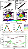Model calculated >70 MeV proton fluxes (with g_b function, $H_{\min} (L, α_{m})$ ${H}_{{min}}\left(L,{\alpha }_m\right)$ = 100 km, optimal collisional loss coefficients: a = 17.5; z₁ = −50 km, z₂ = 0.351, b =1.170), and their comparisons with the observations by RPS-b (2013) and SEM2/POES (1998–2013). The figures are similar to Figures 6–9.

Figure S3:

Model calculated >70 MeV proton fluxes (with g_h function, $H_{\min} (L, α_{m})$ ${H}_{{min}}\left(L,{\alpha }_m\right)$ = 0 km; optimal collisional loss coefficients:a = 18.0; z₁= −35 km, z₂= 0.362, b = 1.142), and their comparisons with the observations by RPS-b (2013) and SEM2/POES (1998–2013). The figures are similar to Figures 6–9.

Figure S4.

Model calculated >70 MeV proton fluxes (with g_h function and H_min(L, α_m)=100 km, optimal collisional loss coefficients: a = 17.5, z₁ = −50 km, z₂ = 0.351, b= 1.142), and their comparisons with the observations by RPS-b (2013) and SEM2/POES (1998–2013). The figures are similar to Figures 6–9.

Figure S5.

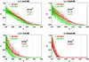Proton flux observations (normalized to the equatorial flux intensity of the shell),y, as a function of B/B₀ in four L shells. Discrete data points: based on observations within the L-shell interval by RPS-b in year 2013 (red: >192 MeV; green: >300 MeV); Solid line: g_b function, computed with value of k indicated (see Equation (6); Vertical dashed line: $H_{\min} (B / B_{0})$ ${H}_{{min}}\left(\enspace {B}/{B}_0\right)\enspace$ = 1000 km, separating the high-altitude region and the low-altitude region of the environment.

Figure S6.

y, proton flux observations (normalized to the equatorial flux intensity of the shell), as a function of $x = (H_{\min} - 50) / (H_{\min, eq} (L) - 50)$ $x=({H}_{{min}}-50)/({H}_{{min},{eq}}(L)-50)\enspace$ in four L shells. Discrete data points: based on observations within the L-shell interval by RPS-b in year 2013 (red: >192 MeV; green: >300 MeV); Solid line: g_h function for the shell (see Equation (8), with the value of η indicated; Vertical dashed line: $H_{\min} (B / B_{0})$ ${H}_{{min}}\left(\enspace {B}/{B}_0\right)$ = 1000 km, separating the high-altitude region and the low-altitude region of the environment.

Current usage metrics show cumulative count of Article Views (full-text article views including HTML views, PDF and ePub downloads, according to the available data) and Abstracts Views on Vision4Press platform.

Data correspond to usage on the plateform after 2015. The current usage metrics is available 48-96 hours after online publication and is updated daily on week days.

Initial download of the metrics may take a while.