| Issue |
J. Space Weather Space Clim.
Volume 16, 2026
|
|
|---|---|---|
| Article Number | 5 | |
| Number of page(s) | 15 | |
| DOI | https://doi.org/10.1051/swsc/2025057 | |
| Published online | 10 February 2026 | |
Research Article
Dynamic modeling of the Earth’s trapped proton environment
1
NASA Langley Research Center, Hampton, VA, USA
2
Old Dominion University, Norfolk, VA, USA
3
NASA Johnson Space Center, Houston, TX, USA
* Corresponding author: This email address is being protected from spambots. You need JavaScript enabled to view it.
Received:
24
January
2025
Accepted:
4
December
2025
Abstract
Context: Reliable prediction of space radiation exposure is critical for safeguarding spacecraft systems and ensuring astronaut health during missions. Accurate radiation risk assessment for space mission requires advanced models of the Earth’s trapped proton environment. These models must reflect temporal variations driven by geomagnetic field evolution and solar cycle modulation. Existing static models, such as AP8 and IRENE-AP9, are not designed to fully capture these evolving conditions. Aims: This paper presents a dynamic modeling method for the prediction of trapped proton fluxes, which incorporate time-dependent variations due to geomagnetic field evolution and solar cycle fluctuations. Methods: The new model consists of two primary components. The first model component calculates flux within a strictly adiabatic geomagnetic system. The second model component quantifies atmospheric collisional losses with solar cycle modulation embedded. The final flux is obtained by applying the collisional loss function to the output of the adiabatic system. Model development is based on cleaned and cross-calibrated satellite observations from the Relativistic Proton Spectrometer (RPS-b) onboard the Van Allen Probes (2013) and the Space Environment Monitor (SEM2) onboard POES satellites (1998–2013). This study utilizes satellite observations of protons with energies greater than 70 MeV. Although the current implementation addresses only this integral energy bin, the methodology is designed to be extensible to a broader energy range. Results: The model reproduces the observations with high accuracy. It captures the northwestward drift of the South Atlantic Anomaly (SAA), solar cycle variations, and hysteresis effects. It also successfully reconstructs the SAA’s 1965 location. Conclusion: The present work demonstrates a model of the integral proton flux above 70 MeV. This model’s physics-based structure effectively represents trapped proton dynamics and provides a foundation for future expansion to full energy spectrum and angular-dependent flux configurations.
Key words: Trapped proton environment modeling / Geomagnetic field / SAA drift / Solar cycle modulation
© X. Xu et al., Published by EDP Sciences 2026
 This is an Open Access article distributed under the terms of the Creative Commons Attribution License (https://creativecommons.org/licenses/by/4.0), which permits unrestricted use, distribution, and reproduction in any medium, provided the original work is properly cited.
1 Introduction
The inner Van Allen Belt, extending from several hundred kilometers to nearly two Earth radii, contains dense population of energetic protons. These arise from a dynamic balance of many processes, including cosmic ray albedo neutron decay (CRAND), solar energetic particle injections, collisional losses, and radial diffusion (Singer, 1958; Farley & Walt, 1971; Farley et al., 1972; Baker et al., 2018; Li & Hudson, 2019). The inner belt comes closest to Earth’s surface in the South Atlantic Anomaly (SAA), where weaker magnetic field strength results from the dipole tilt, field eccentricity, and the offset from Earth’s geodetic center (Stassinopoulos et al., 2015). Intense trapped proton fluxes pose significant radiation risks to spacecraft systems and crew in this environment, making accurate modeling essential for mission planning and risk assessment (Jun et al., 2024).
Gradual geomagnetic field changes, coupled with atmospheric interactions, can significantly alter the trapped proton environment over decades (Heynderickx, 1996). The static AP8 model, based on observations in 1960s (Vette, 1966; Sawyer & Vette, 1976), no longer provides reliable estimates for current missions (Daly et al., 1996; Heynderickx et al., 1996a; Badavi et al., 2006). In addition, solar activity influences both particle source mechanisms and atmospheric interactions. This produces flux variations over the solar cycles which are particularly pronounced at altitudes below 1000 km (Nakano & Heckman, 1968; Dragt, 1971; Huston & Pfitzer, 1998; Huston et al., 1998; Qin et al., 2014; Li et al., 2020). While the AP9-International Radiation Environment Near Earth (IRENE-AP9) model incorporates a broad observational dataset and produces statistical outputs (Ginet et al., 2013; Johnston et al., 2015), at the time of this study, it does not explicitly incorporate solar cycle modulations. This limits the applicability for certain mission radiation risk assessments. This is especially true for human missions to Low Earth Orbit, which tend to last less than a year – a small fraction of the full solar cycle.
Trapped charged particles have three basic motions: gyration around the guiding magnetic field lines, bouncing between mirror points and drifting longitudinally around the Earth. The location of a particle’s drift shell within the radiation belts is commonly characterized by the McIlwain L parameter (McIlwain, 1961). A particle’s equatorial pitch angle α follows the relation  , where B is the local field strength and B0 is the equatorial magnetic field strength of the drift shell. Particles with lower equatorial pitch angles reach lower altitudes. For particles reaching low altitudes (<1000 km), the probability of atmospheric loss increases sharply as altitude decreases. The minimum equatorial pitch angle (αm) required for a particle to complete the longitudinal drifts around the Earth defines the drift loss cone angle. From the perspective of a given location, flux at geomagnetic coordinates (L, α) includes particles with equatorial pitch angle in the range [αm, α].
A key parameter for understanding how the trapped environment responds to secular changes in the geomagnetic field and solar cycle modulations is Hmin, which has two context-dependent but physically unified definitions. For a location, it represents the lowest altitude among its equivalents in geomagnetic coordinates (L, α); for a particle, it is the minimum mirror altitude along its bounce-drift shell. Thus, a particle with drift shell L and equatorial pitch angle α shares the same Hmin (L, α) as the corresponding geomagnetic location.
The residence time of a trapped particle, i.e., the duration from being trapped to loss, is strongly influenced by the atmospheric density along its drift shell. Particles with Hmin in the high-altitude region can remain trapped for extended periods (Selesnick et al., 2007), while those with Hmin in the low altitude region are removed more rapidly due to increased atmospheric interactions. At the so-called atmospheric cutoff altitude (~100 km), the atmospheric density becomes so high that any particles reaching this altitude are lost through collisions.
Ongoing changes in Earth’s geomagnetic field lead to a decreasing trend in Hmin(L, α) (Farley et al., 1972; Lemaire et al., 1990; Selesnick et al., 2007). As a result, particles confined to a given drift shell (L, α) reach lower altitudes at later epochs, leading to an increase in αm and a narrowing pitch angle range [αm, α]. Additionally, particles mirroring at low altitudes within the same drift shell in later epochs are more likely lost due to increased atmospheric interactions. This explains why coupling 1960s observation-based AP8 flux database with the geomagnetic fields of later epoch’s results in unrealistic overestimates of proton flux in the SAA.
Solar cycle modulation of the trapped proton environment is primarily through solar activity-induced atmosphere density changes. Its effect on CRAND is relatively small (Selesnick et al., 2007; Bruno et al., 2021). Heightened solar activity heats Earth’s upper atmosphere, increasing density and collisional loss. Proton flux at low altitudes typically peaks near solar minimum when the atmosphere is coolest. A notable feature at the higher altitudes within the low-altitude region is the hysteresis effect, a delayed response in flux maxima or minima (Huston et al., 1998; Qin et al., 2014). This delay is related to the residence time of particles mirroring at these locations; longer residence times enable the influence of earlier solar conditions to persist and manifest in subsequent observations.
2 Satellite observations for model development
Developing a dynamic model of Earth’s trapped proton environment requires long-term, high-coverage observational data, ideally with high spatial resolution. The Van Allen Probes, launched in September 2012, consisted of twin satellites in highly elliptical orbits, with L-shell values ranging from 1.1 to 7 and altitudes spanning from several hundred kilometers to approximately 30,000 km. They provided extensive coverage of a broad region of the inner belt, including the locations with the highest proton fluxes. In contrast, the POES satellites, orbiting at ~840 km with an inclination of 98°, provided extensive spatial and long-term observations of the SAA region (Evans et al., 2008). Together, these datasets offer valuable insight into the evolving trapped proton environment.
The SEM2 instrument onboard the POES satellite provided proton count data for the >16 MeV, >36 MeV, >70 MeV, and >140 MeV energy channels (Evans & Greer, 2004). The RPS instruments onboard the Van Allen Probes measured protons across a broader energy range of approximately 60 MeV to 2000 MeV using 20 discrete channels (Mazur et al., 2013). As this work focuses on developing a dynamic modeling methodology for the trapped proton environment under an evolving geomagnetic field and varying solar cycle modulations, this analysis is limited to a single energy bin for the >70 MeV trapped protons. The POES dataset used in this work for model development consists of 16-second averaged Level 2 proton count data from NOAA-15 spanning from June 1, 1998, to December 31, 2013.1 The RPS dataset comprises the 1-minute averaged level-2 proton observations from year 2013.2
Extensive data processing is performed to prepare satellite observations for model development. This includes calculating the RPS 1-minute integral flux of >70 MeV protons by summing the product of channel flux and channel energy width; computing yearly averaged >70 MeV POES measurements, binned into 1° longitude by 1° latitude grid boxes for each year from 1998 to 2013; calculating key magnetic field parameters, such as L-shell value, B, α, and Hmin for each data point; removing background contributions from galactic cosmic rays (GCR); and performing cross-calibration between RPS and POES >70 MeV proton flux observations.
The twin RPS instruments (RPS-a and RPS-b), which follow nearly identical orbits, are expected to record similar fluxes. However, significant discrepancies exist between their measurements. Given their similar orbital configurations, these differences are likely due to measurement artifacts rather than the environment (O’Brien et al., 2021). It is found that equatorial fluxes, generally recognized as relatively stable over time, have good agreement between RPS-b observations and the simulations by IRENE-AP9 (V1.57, mean), whereas RPS-a observations are substantially lower. Since the IRENE-AP9 V1.57 fluxes have been extensively cross-checked and calibrated against multiple satellite datasets, RPS-a measurements are excluded from this model development. In summary, only RPS-b and POES measurements are used in this work.
In cross-calibrating the RPS-b and POES measurements for >70 MeV proton fluxes, a technique similar to that used in the IRENE-AP9 model database development (Ginet et al., 2013) is employed. Measurements from RPS-b and POES in 2013 are compared over the same geomagnetic region (L: 1.2–1.5, Hmin > 500 km), where the background noise and GCR contributions are negligible relative to trapped proton fluxes. Analysis indicates that observations from the two satellites are approximately proportional, with POES measurements consistently several times larger. To align the datasets, a downscaling factor of 3.42 is applied to POES observations to match the RPS-b observation. This scale factor is consistent with the value reported in the release note and model validation report of IRENE-AP9 V1.50 (IRENE development team, 2017a, 2017b).
Analysis shows that storm-time solar energetic proton injections have very limited impact on the POES >70 MeV channel, even during highly active periods such as 2003. Therefore, no specific filtering is needed to remove the possible storm-time solar energetic proton injections. The yearly GCR background is extracted from POES observations at locations with Hmin lower than 100 km and is described as a function of L. When subtracting the GCR background from RPS measurements, altitude-dependent variations due to Earth’s shadowing are taken into account.
The geomagnetic parameters for each data point are computed using the International Geomagnetic Reference Field model (IGRF-12; Thébault et al., 2015), with the epoch set to the midpoint of the observed year. The L parameter is computed with the method developed by Kluge (1972) and later modified by Bilitza (1992). The value of B0 is computed as M/L3, where M is Earth’s dipole moment for the given epoch. Hmin is calculated using a quadratic function of ln(B/B0) for a given L-shell, following the approach suggested by Heynderickx et al. (1996b). Instructions and the coefficient tables for calculating Hmin within the internal geomagnetic fields of AP8 and the IGRF-12 geomagnetic fields (covering epochs from 1995 to 2020 at 5-year intervals) are provided in Section 1 of the Supplement.
Figure 1 shows processed >70 MeV proton observations from RPS-b and POES at locations with Hmin above 100 km for year 2013. The left panel uses the (L, B/B0) coordinate system, while the right panel uses (L, Hmin/Hmin,eq) to better visualize the spatial dependence of the flux distribution. Hmin,eq denotes the Hmin of the equatorial locations of the drift shell.
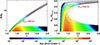 |
Figure 1 Flux observations (>70 MeV protons) by RPS-b and POES (cross-calibrated to RPS-b) in year 2013 at locations with Hmin above 100 km in two different coordinates: Left, (L, B/B0); Right, (L, Hmin/Hmin.eq). Dashed line: Hmin (L) = 1000 km, the reference line to separate the low-altitude region and the high-altitude region of the environment. |
3 Model development
3.1 Modeling framework
The new model represents the trapped proton environment as the product of two primary components: one computes flux within a strictly adiabatic geomagnetic system, and another quantifies atmospheric collisional losses. In the strictly adiabatic system, the proton flux f at a given location (L, X) is expressed as
 (1)
(1)
where the L-shell represents particle’s drift shell and X the bounce location. N0 (L) denotes the flux of the adiabatic system on the geomagnetic equatorial plane. g(L, X) is the geomagnetic field confinement function, which gives the relative flux at the location normalized to N0 (L). X is determined by the approach used in the g function. Two forms of the g function, gb (L, B/B0) and gh(L, Hmin), are independently developed in this work in Section 3.3.
Detailed in Section 3.4, the function r(Hmin,s) provides a scale factor reflecting the impact of collisional loss, where s is a solar cycle activity component. The r function is built upon a scaled atmospheric density function associated with the Hmin of the location. With atmospheric collisional loss accounted for, the proton flux in Earth’s trapped environment is calculated as
![Mathematical equation: $$ f\left(L,X,s\right)={N}_0(L)\cdot g\left(L,X\right)\cdot \left[1-r\left({H}_{\mathrm{min}},s\right)\right]. $$](/articles/swsc/full_html/2026/01/swsc250004/swsc250004-eq3.gif) (2)
(2)
3.2 N0 (L)
Due to the lack of high-quality, cross-calibrated equatorial observations spanning multiple decades, incorporating long-term variation into N0 (L) is currently impractical. With support from both theoretical reasoning and observational evidence, the model treats N0 (L) as time independent.
In a slowly evolving geomagnetic system marked by a weakening dipole moment and contracting drift shells, variations in N0 are expected to be subtle. Lemaire & Singer (2012) projected that fluxes decrease with the dipole weakening, while other studies indicated that shell contraction may increase flux (Farley et al., 1972; Selesnick et al., 2007). These opposing effects likely offset one another to some extent. Given the slow pace of geomagnetic field change relative to the model’s intended time applicability, significant variation in N0 (L) over several decades is unlikely.
Observational data provide further support for the assumption of N0 (L)’s temporal stability. Equatorial measurements remain relatively stable in regions where geomagnetic disturbance is minimal (He et al., 2023). In comparison, N0 has greater stability, since it is unaffected by variations in atmospheric collisional loss driving by geomagnetic field changes or solar modulation.
From a theoretical standpoint, N0 is not directly observable. Equatorial measurements include contributions from particles mirroring at low altitudes, where atmospheric collisional losses reduce flux intensity. As a result, the equatorial measurements inherently include the effects of atmospheric interaction, although such effects are likely minimal at many equatorial locations.
Constructing N0 (L) from observations requires isolating it from atmospheric collisional loss effects. As the systematically available equatorial measurements (denoted as feq) in this work are limited to 2013, N0 (L) in the model is given by
 (3)
(3)
where feq, 2013 (L) is feq of year 2013 and r2013 (Hmin,eq (L), s) is r(Hmin, s) specified for the geomagnetic equatorial locations for year 2013. Extracted from the 2013 observations with B/(B0) < 1.02, feq,2013 is shown in Figure 2.
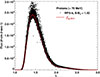 |
Figure 2 Equatorial fluxes (>70 MeV protons) as a function of L-shell value. Discrete data points: observations in year 2013 by RPS-b for locations with B/B0 < 1.02; Solid line in red: feq,2013. |
Replacing the N0 (L) in equation (2) with the expression in equation (3) results in:
![Mathematical equation: $$ f\left(L,X,s\right)=\frac{{f}_{\mathrm{eq},\enspace 2013}(L)}{1-{r}_{2013}\left({H}_{\mathrm{min},{eq}}(L),\enspace {s}\right)}\cdot g\left(L,X\right)\cdot \left[1-r\left({H}_{\mathrm{min}},s\right)\right]. $$](/articles/swsc/full_html/2026/01/swsc250004/swsc250004-eq5.gif) (4)
(4)
This formulation is subsequently used to fit the observational data during the model development and serves as the basis for constructing the g and r functions.
3.3 Geomagnetic field confinement functions
This section presents the derivation and numerical formulations of the gb (L, B/B0) and gh(L, Hmin) functions, which compute the relative flux at a given location, normalized to N0 (L), within a strictly adiabatic magnetic system.
A gb (L, B/B0) function
The distribution of trapped particles along the field line is highly dependent on the local magnetic intensity. The local flux, denoted J(L, B), can be computed by integrating contributions from particles with equatorial pitch angle in the range of [αm, α]. A commonly used equatorial pitch angle distribution (PAD) form is [sin(αi)]k(L) (Selesnick et al., 2014; Ni et al., 2015; Shi et al., 2016; Roussos et al., 2018; Xu et al., 2019; Greeley et al., 2021). Accordingly, with the equatorial flux at 90° for a given L-shell denoted as j0 (L), the local flux J(L, B) is calculated using the integral formulation provided in Roederer (1970):
![Mathematical equation: $$ J\left(L,B\right)=4\frac{B}{{B}_0}\underset{\mathrm{cos}\left(\alpha \right)}{\overset{\mathrm{cos}\left({\alpha }_m\right)}{\int }}{j}_0{(L)\cdot \left[\mathrm{sin}\left({\alpha }_i\right)\right]}^{k(L)}\cdot \frac{\mathrm{cos}\left({\alpha }_i\right)}{\sqrt{1-\frac{B}{{B}_0}\left(1-{\mathrm{cos}}^2\left({\alpha }_i\right)\right)}}d\left(\mathrm{cos}\left({\alpha }_i\right)\right). $$](/articles/swsc/full_html/2026/01/swsc250004/swsc250004-eq6.gif) (5)
(5)
Function gb (L, B/B0), the relative flux normalized to N0 (L), is calculated by J(L, B)/N0 (L). Since N0 (L) = J(L, B0), function gb (L, B/B0) is given as
 (6)
(6)
It is worth noting that in an evolving geomagnetic field, the time dependence in gb (L, B/B0) is obtained through the time variation in αm (L).
Calculations using equation (6) require the value of αm of the shell, or equivalently, the corresponding magnetic field strength Bm. For a particle to complete the longitudinal drift around the Earth, the minimum altitude of its gyration-bounce-drift orbit is required to be above Earth’s surface. Accurate determination of Bm involves a three-dimensional search for the lowest mirroring point where the vertical component of the particle’s gyration radius equals Hmin(L, αm). Trapped protons come closest to Earth’s surface in the SAA region. To simplify the analysis, an approximation is used for the vertical component of the gyration radius near Earth’s surface within this region. Using the formulation in Armstrong et al. (1990), the gyration radius of a 100 MeV proton at the Earth’s surface in the SAA is approximately 60 km. Slightly smaller than the full gyration radius, the vertical component is approximated as 50 km. Accordingly, Hmin(L, αm) = 50 km is used to estimate the corresponding Bm.
Since the integration over the equatorial pitch angle range [αm, α] cannot be performed analytically, a numerical approach is used in this work. To minimize uncertainties, the integration is carried out using a fine step size; specifically, one hundredth of the width of the equatorial pitch angle range [αm, α] is used in the calculations presented in this work.
To determine the geomagnetic location dependence of component k, analysis of high-altitude RPS-b observations indicates that, for a given particle energy, modeling k as a function of L-shell alone is sufficient (see Fig. 3). Accordingly, constructing the gb function for >70 MeV protons reduces to numerically specifying the component k(L).
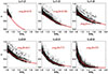 |
Figure 3 y, >70 MeV proton flux observations normalized to feq(L), as a function of B/B0 in six L shells of the IGRF field for year 2013. Discrete data points: based on observations by RPS-b at high altitudes (Hmin > 1000 km) in year 2013; Solid line: gb function, computed with value of k indicated (see Eq. (6)). |
B gh (L, Hmin) function
The g function has a value of 1.0 at the equatorial location. As the location moves along the field line toward Earth’s surface, it decreases gradually and reaches zero at the location where the corresponding equatorial pitch angle α equals αm. To capture this behavior, a power-law function is deliberately chosen:
 (7)
(7)
Preliminary analysis based on RPS-b observations indicates that, for a given particle energy, it is adequate to model the exponent η as a function of L-shell alone (see Fig. 4). With Hmin (L, αm) approximated as 50 km, as discussed in Section 3.3A, the gh (L, Hmin) equation simplifies to:
 (8)
(8)
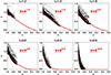 |
Figure 4 y, >70 MeV proton flux observations normalized to feq(L), as a function of x = (Hmin − 50)/(Hmin,eq (L) − 50) in six L shells of IGRF field for year 2013. Discrete data points: based on observations by RPS-b at high altitudes (Hmin > 1000 km) in year 2013; Solid line: gh function of the shell (see Eq. (8)). |
The remaining task in building the gh function for >70 MeV protons is to numerically determine the component η(L).
3.4 Collisional loss function with solar cycle modulations
This section presents the derivation and numerical formulation of the collisional loss function r. Using collision theory (Pechukas, 1976), collisional loss rate is quantified by the following function:
 (9)
(9)
In the equation, a is a collisional interaction coefficient and ρ is a scaled atmospheric density that depends on the Hmin of the location and solar cycle activity parameter s. The function r(Hmin, s) increases with ρ, ranging from 0 (no collisional loss on local flux) to 1 (complete particle loss).
The scaled atmospheric density component ρ(Hmin, s) is computed using a formulation similar to those used for estimating atmospheric density at satellite altitudes (Walker, 1964; Martin, 1965; Jacchia, 1970; Emmert, 2015):
![Mathematical equation: $$ \rho \left({H}_{\mathrm{min}},s\right)={e}^{-\left[{\left(\frac{{H}_{\mathrm{min}}}{{z}_1+{z}_2\bullet s}\right)}^b\right]}. $$](/articles/swsc/full_html/2026/01/swsc250004/swsc250004-eq11.gif) (10)
(10)
In this expression, the solar modulation effect is incorporated into the atmospheric scale height term, z1 + z2s, where both z1 and z2 are positive-valued parameters.
The solar radio flux at 10.7 cm, known as F10.7 and having a long-standing history in atmospheric density modeling at satellite altitudes (Hedin, 1991; Bilitza, 2001; Picone et al., 2002; Emmert, 2015), is employed here as a proxy for tracking solar cycle activity levels.3 Particles mirroring at locations with higher Hmin generally have longer residence times than those mirroring at low altitudes. As a result, the flux at locations with higher Hmin in the SAA region is influenced by solar modulation effects over a longer temporal window. To incorporate this effect, the solar activity level parameter s is calculated as the average F10.7 over a period of m months preceding the target epoch, where m depends on Hmin. Specifically,
 (11)
(11)
This dependency of m on Hmin is empirically derived from POES observations of >70 MeV protons. Complete evaluation of the collisional loss requires specifying the coefficients a, b, z1, and z2.
3.5 Completion of the model for >70 MeV protons
The final step in model development for >70 MeV protons is to specify the pitch angle distribution exponent k(L) needed to calculate gb, the altitude dependence exponent η(L) needed to calculate gh, and the coefficient a, b, z1, and z2 required for the collisional loss function r(Hmin,s). This is accomplished by fitting equation (4) to the observational data from RPS-b (2013) and POES/SEM2 (1998–2013).
The optimization process involves three main steps. First, the numerical forms of k(L) and η(L), along with preliminarily coefficients estimates, are derived from RPS-b 2013 observations from locations with Hmin > 1000 km, where the impact of collisional loss is low. Second, using the k(L) and η(L) from previous step, the collisional interaction coefficient a and the atmospheric scale height coefficients z1, and z2 are estimated by fitting to the POES/SEM2 1998–2013 observations, with the exponent b fixed at 1.0. Finally, all coefficients in the k(L), η(L), and r(Hmin, s) functions are refined through fine-tuning to fit the satellite observations.
The forms of k(L) and η(L) are empirical, chosen for their effectiveness in reproducing the observation data. The resulting optimal expressions are:
 (12)
(12)
and
 (13)
(13)
The optimal values for the coefficients used in the collisional loss function for >70 MeV proton flux are summarized in Table 1.
Coefficient list for the calculation of r(Hmin,s).
Analysis of the model simulations reveals that the optimal gb and gh functions for >70 MeV protons yield very similar values for shells with L < 2.0, with some noticeable differences emerging in shells with L > 2.0. A representative comparison of the gb and gh functions for year 2013 is presented in Figure 5. Analysis also shows that the slight difference in the optimal b values between the r functions for gb and gh results only minor differences between the two r functions.
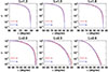 |
Figure 5 Comparison of the optimal g functions for >70 MeV protons (red solid line: gb; dashed blue line: gh), as a function of the corresponding equatorial pitch angle α of a geomagnetic location, evaluated in six L shells of IGRF field for 2013. |
While 50 km is a reasonable approximation for Hmin (L, αm), sensitivity tests using 0 km and 100 km are performed to investigate how the Hmin (L, αm) approximation impacts the model’s performance. The results indicate that the flux uncertainties introduced by the approximation are relatively small and primarily confined to low altitude locations. Since collisional loss to the atmosphere has a greater impact on fluxes at the low altitudes, the uncertainties are largely absorbed into the r function. Tuning the r function yields comparable model performance in fitting the observations (Figs. S1–S4). Overall, the model is robust to reasonable variations in the assumed value of Hmin (L, αm).
4 Results
This section compares model-calculated >70 MeV proton fluxes or the times and locations of the satellite measurements. In general, the model calculations agree well with satellite observations from RPS-b (2013) and POES (1998–2013), as shown in the scatter plots of Figure 6, where the coefficient of determination (R2) is provided as a measure of goodness of fit. Model outputs, using either the gb or gh function along with the respective r function, have similar performances.
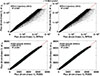 |
Figure 6 Comparison of model calculated >70 MeV proton fluxes with observations. Left panels: model calculations with gb function. Right panels: model calculations with gh function; Upper panels: fluxes along the 1-minute RPS-b trajectory in year 2013; Lower panels: fluxes at POES satellite altitude for each year between 1998–2013; y = x: the perfect fit line (red); Coefficients of determination R2 are denoted. |
Fluxes in the low-altitude region exhibit strong spatial gradients. To assess model performance, Figure 7 presents the >70 MeV trapped proton fluxes measured by POES in geographic coordinates for the years 2003 and 2010 (one year after the solar activity extremes), with Hmin and L overlaid. The new dynamic model accurately locates the flux center and effectively captures the spatial gradient and solar modulation induced variation.
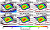 |
Figure 7 >70 MeV proton fluxes in the year following solar activity extremes at POES altitude in the geographic coordinate, with L (1.2, 1.35, 2.0, and 4.0, in black) and Hmin (100 km, 300 km, and 600 km, in red) isolines overlaid, and with the flux peaking area marked by the lines crossing at [50° W, 26° S]; Left panels: observations by POES; Middle panels: model calculations with gb function; Right Panels: model calculations with gh function. |
Fluxes in the low-altitude region are particularly sensitive to changes in the geomagnetic field and solar cycle modulation due to their interaction with the neutral atmosphere. To evaluate the model’s capability in capture these flux changes, Figure 8 presents model-calculated yearly flux profiles from 1998 to 2013 at POES altitude along 26° S latitude and 50° W longitude, compared with corresponding POES observations. The new dynamic model successfully reproduces the variations over the 16-year span, and notably it accurately represents the yearly northwestward drift. This provides strong evidence of model’s ability to account for both the evolving geomagnetic field and the solar modulation.
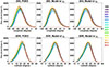 |
Figure 8 Yearly >70 MeV proton fluxes crossing 26° S (upper panels) and 50° W (lower panels) at POES orbit altitude during 1998–2013 (year color coded). Left panels: POES observations; Middle panels: model calculations with gb function; Right panels: model calculations with gh function. |
To examine the model’s ability to capture solar modulation-induced time variations, including the hysteresis effects, Figure 9 presents monthly F10.7 indices alongside the observed and model-simulated fluxes averaged over three Hmin zones. Among the three zones, the hysteresis effect is most pronounced in the zone with the highest Hmin. As the solar activity reaches a maximum in 2002 or a minimum in 2009, fluxes in the Hmin >750 km zone do not reach the corresponding minimum or maximum until one or two years later. Although some uncertainties are evident in the high-altitude zone, the new model captures the time variations in the low-altitude region well, including the hysteresis effects.
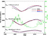 |
Figure 9 Yearly variations in >70 MeV proton flux at POES altitude, averaged over the locations with L in the range of 1.25–1.6 for three Hmin zones; Observations by POES (black); model calculations with gb (solid red); model calculations with gh (blue dashed); Monthly F10.7 variation (green). |
Although the model has demonstrated strong performance in reproducing the long-term POES observations, a thorough validation on longer timescales is constrained by the lack of high-quality observations across extended periods. To partially address this, the model’s capability to predict the northwestward drift of the low-altitude region is evaluated through its ability to reconstruct the SAA location in the AP8-MIN epoch, which corresponds to one of the earliest periods with systematic observations of the trapped proton belt. Figure 10 presents a comparison of model-simulated flux distributions at the POES altitude for the AP8-MIN epoch (1965) and for the year 2013, alongside AP8-MIN model outputs and POES 2013 observations, respectively. The results show that the new model effectively reproduces the drift of the low altitude region over the ~50-year span. For the 1965 environment simulations, the model captures the overall flux distribution well. The differences between the new model and AP8-MIN are largely due to the low spatial resolution of the AP8-MIN model and the lack of cross-calibration between RPS-b and the observing instruments used in the AP8-MIN model construction.
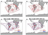 |
Figure 10 Northwestward drift of the low-altitude region of the SAA from 1965 to 2013. The plots show the contour lines of >70 MeV proton flux intensities at 840 km from: a) AP8-MIN; b) POES 2013 observations; c) model calculations (solid red line: with gb; dashed blue: with gh) for year 1965; d) model calculations for year 2013 (solid red line: with gb; dashed blue line: with gh). |
To evaluate the model’s predictive capability beyond its development period, Figure 11 compares model-projected >70 MeV proton fluxes at POES altitude with yearly averaged POES/SEM2 observations for 2020 (solar minimum) and 2024 (solar maximum). The POES observations, available as raw Level 1a data,4 are processed using the same method outlined in Section 2, including a consistent scaling factor. The model reproduces the geographic distribution of >70 MeV proton fluxes with high fidelity. Direct comparisons between model simulations and POES observations yield correlation coefficients of 0.998 for 2020 and 0.985 for 2024, indicating excellent spatial agreement. Despite this strong correlation, the model underestimates by approximately 10%. The origin of this bias remains uncertain and may stem from limitations in the model or from the observational dataset. For example, differences in data processing levels or degradation of instrument hardware, as NOAA-15 approaches the end of its operational life, could distort the measurement data. For reference, AP8-MIN and AP8-MAX simulations (shifted 5° northward and 15° westward to match the observed flux peak), as well as IRENE-AP9 simulations (version 1.57, mean mode), are also compared with POES observations for both years.
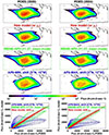 |
Figure 11 >70 MeV proton fluxes in year 2020 (solar minimum) and year 2024 (approximately solar maximum) at POES altitude. upper row: POES observations; second row: simulations by the new method; third row: simulations by IRENE-AP9 (V1.57, mean mode); forth row: simulation by AP8-MIN and AP8-MAX, with geomagnetic field shifting (5° N, 15° W) to match the flux peak location; bottom row: scatter plots to compare model simulations with POES observations. |
5 Discussion
High-performance trapped proton environment models are essential for mission radiation risk analysis. Modeling the low-altitude region is particularly challenging due to its strong spatial and temporal dependencies, driven by geomagnetic field changes and solar modulation, and further complicated by the particle-atmosphere interactions.
This work introduces a framework for a dynamic model composed of two primary components. The first calculates flux within a strictly adiabatic geomagnetic system, constructed from two key elements: N0 (L), representing the equatorial fluxes of a strictly adiabatic geomagnetic system, and the g function, which provides the relative flux normalized to N0 (L). The second primary component quantifies atmospheric collisional loss effects via the r function. The resulting flux is expressed as the product of N0 (L), the g function, and the attenuation factor 1 − r. The IGRF-12 model is used for the geomagnetic field description. Observations from POES (1998–2013) and RPS-b (2013) are used in model construction. N0 (L), derived from RPS-b data for the year 2013, is treated as time-invariant.
The model successfully reproduces the key observational features, such as the northwestward drift, solar cycle variations, and hysteresis effects. This indicates that the model framework and the formulation of the g and r functions effectively capture the underlying mechanisms. The model’s ability to predict the flux peak location and overall flux distributions in the low-altitude region for the AP8 epoch further supports its validity and suggests its applicability for predictions for future decades.
The trapped proton environment consists of protons over a wide range of energies and is highly directional, particularly at low altitudes. The applicability of the current modeling approach to a wider energy range, as well as its possible extension to a directional model, is discussed here.
Particle angle distribution in a strictly adiabatic system is governed by the radial and pitch angle diffusion processes (Roederer, 1970). Based on a widely used formulation for PAD, the term j0 (L)[sin(αi)]k(L) is expected to remain valid across a broad energy range, while k(L) is expected to vary with energy. Such expectations are supported by the analysis presented in Figure S5. Moreover, with the PAD function embedded, the gb function is well-suited for future extension from an omnidirectional model to a directional model.
Compared to the gb function, the gh function has a very simple structure. Preliminary analysis of the RPS-b observations confirms that the structure of the gh function performs well across a wider range of particle energies, with energy dependence encapsulated in the component η (see Fig. S6 for an example). The gh function does not incorporate flux directionality and that constrains its applicability in a directional model. However, its simpler structure offers a computational advantage. The gb function requires numerical integration over the pitch angle range [αm, α] with small step sizes and needs the value of αm (or equivalently Bm) calculated, which is time-dependent and varies with L-shell. In contrast, the gh is analytical and does not require αm or Bm, as the relevant information is encoded in Hmin (L, αm), which can be approximated as 50 km and yields comparable modeling performance. Whether this performance persists across a wider energy range remains to be explored in the development of a full-spectrum model. If confirmed, gh could serve as a fast and effective replacement for gb when an omni-directional model is sufficient.
Collisional loss significantly contributes to flux directionality, with stronger attenuation in directions where particles mirror at lower altitudes. In a directional environment model, this directionality can be introduced via direction-associated Hmin. Energy dependence in the r function is expected, as the gyroradius of trapped protons increases with proton energy, and further analysis is needed to quantify and incorporate it. Nonetheless, the general form of the r function, grounded in collisional theory, is expected to perform well across a broad energy range and for differential fluxes.
This modeling approach has certain limitations due to its simplifying assumptions, and several temporal variations are not accounted for. First, the Earth’s magnetic field is a sum of the internal and external fields. Substantial field changes during geomagnetic storms can lead to flux variations, most pronounced in shells near the outer edge of the radiation belt. Second, some solar activity-related processes are not included in the model. These include solar proton injections, which primarily affect fluxes below a few tens of MeV in the outer shells, and solar modulation of CRAND, whose effects are largely confined to low altitudes in very low-L shells (Selesnick et al., 2007; Bruno et al., 2021). Additionally, the slow change in N0 induced by the geomagnetic field is not considered.
6 Conclusion
Accurate simulation of Earth’s trapped proton environment, with variations driven by geomagnetic field evolution and solar modulation incorporated, is essential for effective radiation risk management. Existing static models, such as AP8 and IRENE-AP9, do not fully capture these time-dependent dynamics. To address this limitation, this work introduces a dynamic modeling framework that incorporates effects of the geomagnetic field evolution and solar cycle modulation.
The model integrates two key components: one describing proton fluxes confined within a strictly adiabatic geomagnetic system, and another quantifying atmospheric collisional losses. Solar cycle modulation is embedded directly into the loss formulation. The model is currently parameterized for >70 MeV protons, using cleaned and cross-calibrated satellite observations from RPS-b (2013) and POES (1998–2013). While some uncertainties remain at higher altitudes within the SAA region, the model effectively reconstructs the observations, including the northwestward drift of the SAA, solar modulation effects, and hysteresis. It also successfully reconstructs the 1965 location of the SAA.
These results demonstrate that the model’s physics-based structure effectively captures the influence of underlying physical mechanisms on the trapped proton environment. Although the current fitting is limited to one single energy channel, the framework is designed to be extensible to a broader energy range and directional flux configurations, providing a robust foundation for future development.
Acknowledgments
We gratefully acknowledge assistance from the IRENE-AP9 development team, especially William Johnston of the Air Force Research Laboratory, who helped with the IRENE-AP9 model installation by providing valuable and technical input. The editor thanks Daniel Heynderickx and an anonymous reviewer for their assistance in evaluating this paper.
Declaration of AI-assisted technologies in the writing process
During the preparation of this work the authors used Microsoft Copilot to review the grammar and language. After using this tool, the authors reviewed and edited the content as needed and take full responsibility for the content of the publication.
Funding
A significant part of this work was performed under NASA’s Advanced Exploration System RadWorks project with support from the Durability, Damage Tolerance, and Reliability Branch of NASA Langley Research Center.
Data availability statement
F10.7 solar indices used in this study are available from https://lasp.colorado.edu/lisird/data/noaa_radio_flux, hosted at Interactive Solar Irradiance Datacenter, Laboratory for Atmospheric and Space Physics, University of Colorado Boulder.
POES/SEM2 data used in this study are available from https://www.ngdc.noaa.gov/stp/satellite/poes/dataaccess.html, hosted at National Geophysical Data Center of National Oceanic and Atmospheric Administration (NOAA).
Van Allen Probes RPS 1-minute averaged Level‐2 data of year 2013 are available from https://cdaweb.gsfc.nasa.gov/pub/data/rbsp/rbspb/l2/rps/psbr-rps-1min/2013/, hosted at the Coordinated Data Analysis Web, NASA Goddard Space Flight Center.
Supplementary material
Section 1. Hmin calculations. Access Supplementary Material
Section 2. Figures.
 |
Figure S1. Model calculated >70 MeV proton fluxes (gb function, |

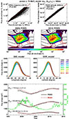 |
Figure S2. Model calculated >70 MeV proton fluxes (with gb function, |

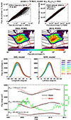 |
Figure S3: Model calculated >70 MeV proton fluxes (with gh function, |

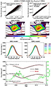 |
Figure S4. Model calculated >70 MeV proton fluxes (with gh function and Hmin(L, αm)=100 km, optimal collisional loss coefficients: a = 17.5, z1 = −50 km, z2 = 0.351, b= 1.142), and their comparisons with the observations by RPS-b (2013) and SEM2/POES (1998–2013). The figures are similar to Figures 6–9. |
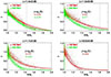 |
Figure S5. Proton flux observations (normalized to the equatorial flux intensity of the shell),y, as a function of B/B0 in four L shells. Discrete data points: based on observations within the L-shell interval by RPS-b in year 2013 (red: >192 MeV; green: >300 MeV); Solid line: gb function, computed with value of k indicated (see Equation (6); Vertical dashed line: |

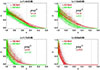 |
Figure S6. y, proton flux observations (normalized to the equatorial flux intensity of the shell), as a function of |


Downloaded from https://cdaweb.gsfc.nasa.gov/pub/data/rbsp/rbspb/l2/rps/psbr-rps-1min/2013/.
Data downloaded from https://lasp.colorado.edu/lisird/data/noaa_radio_flux.
References
- Armstrong, TW, Colborn BL, Watts J. 1990. Characteristics of Trapped Proton Anisotropy at Space Station Freedom Altitudes. Tech. Rep., SAIC90/1474. Science Applications International Corporation. https://ntrs.nasa.gov/api/citations/19910006640/downloads/19910006640.pdf. [Google Scholar]
- Badavi, FF, West KJ, Nealy JE, Wilson JW, Abrahms BL, Luetke NJ. 2006. A dynamic/anisotropic low Earth orbit (LEO) ionizing radiation model. NASA-TP-214533. https://spaceradiation.larc.nasa.gov/nasapapers/2006/20070004574.pdf. [Google Scholar]
- Baker, DN, Erickson PJ, Fennell JF, Foster JC, Jaynes AN, et al. 2018. Space weather effects in the Earth’s radiation belts. Space Sci Rev 214: 17. https://doi.org/10.1007/s11214-017-0452-7. [Google Scholar]
- Bilitza, D. 1992. Solar-terrestrial models and application software. Planet Space Sci 40 (4): 541–544. https://doi.org/10.1016/0032-0633(92)90173-L. [Google Scholar]
- Bilitza, D. 2001. International Reference Ionosphere 2000. Radio Sci 36 (2): 261–275. https://doi.org/10.1029/2000RS002432. [CrossRef] [Google Scholar]
- Bruno, A, Martucci M, Cafagna FS, Sparvoli R, Adriani O, et al. 2021. Solar-cycle variations of South Atlantic anomaly proton intensities measured with the PAMELA Mission. Astrophys J Lett 917: L21. https://doi.org/10.3847/2041-8213/ac1a74. [Google Scholar]
- Daly, EJ, Lemaire J, Heynderickx D, Rodgers DJ. 1996. Problems with models of the radiation belts. IEEE Trans Nucl Sci 43 (2): 403–415. https://doi.org/10.1109/23.490889. [Google Scholar]
- Dragt, AJ. 1971. Solar cycle modulation of the radiation belt proton flux. J Geophys Res 76 (10): 2313–2344. https://doi.org/10.1029/JA076i010p02313. [Google Scholar]
- Emmert, JT. 2015. Thermospheric mass density: A review. Adv Space Res 56 (5): 773–824. https://link.springer.com/article/10.1007/s11214-017-0452-7. [CrossRef] [Google Scholar]
- Evans, D, Greer MS. 2004. Polar orbiting environmental satellite space environment monitor-2. Instrument descriptions and archive data documentation. NOAA Tech. Mem. 1.4. https://ngdc.noaa.gov/stp/satellite/poes/docs/SEM2Archive.pdf. [Google Scholar]
- Evans, D, Garrett H, Jun I, Evans R, Chow J. 2008. Long-term observations of the trapped high-energy proton population (L < 4) by the NOAA Polar Orbiting Environmental Satellites (POES). Adv Space Res 41 (8): 1261–1268. https://doi.org/10.1016/j.asr.2007.11.028. [Google Scholar]
- Farley, TA, Walt M. 1971. Source and loss processes of protons of the inner radiation belt. J Geophys Res 76 (34): 8223–8240. https://doi.org/10.1029/JA076i034p08223. [Google Scholar]
- Farley, TA, Kivelson MG, Walt M. 1972. Effects of the secular magnetic variation on the distribution function of inner-zone protons. J Geophys Res 77 (31): 6087–6092. https://doi.org/10.1029/JA077i031p06087. [Google Scholar]
- Ginet, GP, O’Brien TP, Huston SL, Johnston WR, Guild TB, et al. 2013. AE9, AP9 and SPM: New models for specifying the trapped energetic particle and space plasma environment. Space Sci Rev 179: 579–615. https://doi.org/10.1007/s11214-013-9964-y. [CrossRef] [Google Scholar]
- Greeley, AD, Kanekal SG, Sibeck DG, Schiller Q, Baker DN. 2021. Evolution of pitch angle distributions of relativistic electrons during geomagnetic storms: Van Allen Probes observations. J Geophys Res Space Phys 126: e2020JA028335. https://doi.org/10.1029/2020JA028335. [Google Scholar]
- He, Z, Xu J, Dai L, Wang C, Chen T, et al. 2023. Characteristics of high-energy protons in the equatorial plane of inner radiation belt observed by Van Allen Probes. J Geophys Res Space Phys 128: e2023JA031484. https://doi.org/10.1029/2023JA031484. [Google Scholar]
- Hedin, AE. 1991. Extension of the MSIS thermosphere model into the middle and lower atmosphere. J Geophys Res 96 (A2): 1159–1172. https://doi.org/10.1029/90JA02125. [Google Scholar]
- Heynderickx, D. 1996. Comparison between methods to compensate for the secular motion of the South Atlantic Anomaly. Radiat Meas 26 (3): 369–373. https://doi.org/10.1016/1350-4487(96)00056-X. [Google Scholar]
- Heynderickx, D, Lemaire J, Daly EJ, Evans H. 1996a. Calculating low-altitude trapped particle fluxes with the NASA Models AP-8 and AE-8. Radiat Meas 26: 947–952. https://doi.org/10.1016/S1350-4487(96)00096-0. [Google Scholar]
- Heynderickx, D, Kruglanski M, Lemaire J, Daly EJ. 1996b. Trapped proton modelling at low altitude. In: ESA-SP 392: Symposium Proceedings on Environment Modelling for Space-based Applications, Vol. 392, pp. 75–80. https://orfeo.belnet.be/handle/internal/5499. [Google Scholar]
- Huston, S, Pfitzer K. 1998. Space environment effects: Low-altitude trapped radiation model. Tech. Rep. NASA/CR-1998-208593, NASA/MSFC. https://ntrs.nasa.gov/api/citations/19980222262/downloads/19980222262.pdf. [Google Scholar]
- Huston, S, Kuck G, Pfitzer K. 1998. Solar cycle variation of the low-altitude trapped proton flux. Adv Space Res 21 (12): 1625–1634. https://doi.org/10.1016/S0273-1177(98)00005-2. [Google Scholar]
- IRENE (AE9/AP9/SPM) Development Team. 2017a. IRENE:AE9/AP9/SPM radiation environment model release notes, Version 1.50.001. https://www.vdl.afrl.af.mil/programs/ae9ap9/files/package/Ae9Ap9_v1_50_001_ReleaseNotes.pdf. [Google Scholar]
- IRENE (AE9/AP9/SPM) Development Team. 2017b. AP9 V1.50.001 Model Validation Summary Report. https://www.vdl.afrl.af.mil/programs/ae9ap9/files/package/AP9_V1.50.001_Validation_Summary.pdf. [Google Scholar]
- Jacchia, LG. 1970. New static models of the thermosphere and exosphere with empirical temperature profiles. SAO Special Report 313. https://ntrs.nasa.gov/api/citations/19700027590/downloads/19700027590.pdf. [Google Scholar]
- Johnston, WR, O’Brien TP, Huston SL, Guild TB, Ginet GP. 2015. Recent updates to the AE9/AP9/SPM radiation belt and space plasma specification model. IEEE Trans Nucl Sci 62: 2760–2766. https://ieeexplore.ieee.org/document/7317603. [CrossRef] [Google Scholar]
- Jun, I, Garrett H, Kim W, Zheng Y, Fung SF, et al. In press. A review on radiation environment pathways to impacts: Radiation effects, relevant empirical environment models, and future needs. Adv Space Res. https://doi.org/10.1016/j.asr.2024.03.079. [Google Scholar]
- Kluge, G. 1972. Direct computation of the magnetic shell parameter. Comput Phys Commun 3 (1): 31–35. https://doi.org/10.1016/0010-4655(72)90051-3. [Google Scholar]
- Lemaire, J, Daly EJ, Vette JI, McIlwain CE, McKenna-Lawlor S. 1990. Secular variations in the geomagnetic field and calculations of future low altitude radiation environments. In: ESA-WPP 23: Proceedings of the ESA Workshop on Space Environment Analysis, ESTEC, Noordwijk, The Netherlands. 23. https://orfeo.belnet.be/handle/internal/5715. [Google Scholar]
- Lemaire, JF, Singer SF. 2012. What happens when the geomagnetic field reverses? In: D, Summers, Mann IR, Baker DN, Schulz MDynamics of the Earth’s Radiation Belts and Inner Magnetosphere. Geophysical Monograph Series, Vol. 199, American Geophysical Union, pp. 355–364. https://doi.org/10.1029/2012GM001307. ISBN:9780875904894. [Google Scholar]
- Li, W, MK Hudson. 2019. Earth’s Van Allen radiation belts: From discovery to the Van Allen Probes era. J Geophys Res Space Phys, 124: 8319–8351. https://doi.org/10.1029/2018JA025940. [CrossRef] [Google Scholar]
- Li, X, Xiang Z, Zhang K, Khoo L, Zhao H, et al. 2020. New insights from long‐term measurements of inner belt protons (10s of MeV) by SAMPEX, POES, Van Allen Probes, and simulation results. J Geophys Res Space Phys 125: e2020JA028198. https://doi.org/10.1029/2020JA028198. [Google Scholar]
- Martin, JJ. 1965. Evaluation of the atmospheric density scale height. J Geophys Res 70 (20): 5328–5329. https://doi.org/10.1029/JZ070i020p05328. [Google Scholar]
- Mazur, J, Friesen L, Lin A, Mabry D, Katz N, et al. 2013. The Relativistic Proton Spectrometer (RPS) for the radiation Belt storm probes mission. Space Sci Rev 179: 221–261. https://doi.org/10.1007/s11214-012-9926-9. [Google Scholar]
- McIlwain, CE. 1961. Coordinates for mapping the distribution of magnetically trapped particles. J Geophys Res 66: 3681–3691. https://doi.org/10.1029/JZ066i011p03681. [CrossRef] [Google Scholar]
- Nakano, G, Heckman H. 1968. Evidence for solar-cycle changes in the inner-belt protons. Phys Rev Lett 20 (15): 806–809. https://journals.aps.org/prl/pdf/10.1103/PhysRevLett.20.806. [Google Scholar]
- Ni, B, Zou Z, Gu X, Zhou C, Thorne RM, et al. 2015. Variability of the pitch angle distribution of radiation belt ultra-relativistic electrons during and following intense geomagnetic storms: Van Allen Probes observations. J Geophys Res Space Phys 120 (6): 4863–4876. https://doi.org/10.1002/2015JA021065. [Google Scholar]
- O’Brien, TP, Looper MD, Mazur JE, Mazur EL. 2021. Relativistic proton spectrometer flux determination and data products. Aerospace Technical Report ATR-2021-02018. https://spdf.gsfc.nasa.gov/pub/data/rbsp/documents/rps/ATR-2021-02018-Relativistic_Proton_Spectrometer_Flux_Determination_and_Data_Products.pdf. [Google Scholar]
- Pechukas, P. 1976. Statistical approximations in collision theory. In: WH, Miller (Ed.), Dynamics of molecular collisions. modern theoretical chemistry. Vol. 2, Springer, Boston, MA. https://doi.org/10.1007/978-1-4757-0644-4_6. Online ISBN: 978-1-4757-0644-4. [Google Scholar]
- Picone, J, Hedin A, Drob D, Aikin A. 2002. NRLMSISE-00 empirical model of the atmosphere: Statistical comparisons and scientific issues. J Geophys Res 107: A12. https://doi.org/10.1029/2002JA009430. [Google Scholar]
- Qin, M, Zhang X, Ni B, Song H, Zou H, et al. 2014. Solar cycle variations of trapped proton flux in the inner radiation belt. J Geophys Res Space Phys 119 (12): 9658–9669. https://doi.org/10.1002/2014JA020300. [Google Scholar]
- Roederer, JG. 1970. Dynamics of geomagnetically trapped radiation. Springer-Verlag Berlin, Heidelberg. ISBN 978-3-642-49300-3. https://doi.org/10.1007/978-3-642-49300-3. [Google Scholar]
- Roussos, E, Kollmann P, Krupp N, Kotova A, Regoli L, et al. 2018. A radiation belt of energetic protons located between Saturn and its rings. Science (New York, NY) 362 (6410): eaat1962. https://doi.org/10.1126/science.aat1962. [Google Scholar]
- Sawyer, DM, Vette JI. 1976. AP-8 trapped proton environments for solar maximum and solar minimum. NSSDC/WDC-A-R&S 76–06. https://ntrs.nasa.gov/api/citations/19770012039/downloads/19770012039.pdf. [Google Scholar]
- Selesnick, RS, Baker DN, Jaynes AN, Li X, Kanekal SG, et al. 2014. Observations of the inner radiation belt: CRAND and trapped solar protons. J Geophys Res Space Phys 119: 6541–6552. https://doi.org/10.1002/2014JA020188. [Google Scholar]
- Selesnick, RS, Looper MD, Mewaldt RA. 2007. A theoretical model of the inner proton radiation belt. Space Weather 5 (4): S04003. https://doi.org/10.1029/2006SW000275. [Google Scholar]
- Shi, R, Summers D, Ni B, Manweiler JW, Mitchell DG, et al. 2016. A statistical study of proton pitch angle distributions measured by the Radiation Belt Storm Probes Ion Composition Experiment. J Geophys Res Space Phys 121: 5233–5249. https://doi.org/10.1002/2015JA022140. [Google Scholar]
- Singer, SF. 1958. Trapped Albedo theory of the radiation belt. Phys Rev Lett 1: 181–183. https://link.aps.org/doi/10.1103/PhysRevLett.1.181. [Google Scholar]
- Stassinopoulos, EG, Xapsos MA, Stauffer CA. 2015. Forty-Year “Drift” and Change of the SAA. NASA/TM–2015-217547. https://ntrs.nasa.gov/citations/20160003393. [Google Scholar]
- Thébault, E, Finlay CC, Beggan CD, Alken P, Aubert J, et al. 2015. International Geomagnetic Reference Field: the 12th generation. Earth Planet Space 67: 79. https://doi.org/10.1186/s40623-015-0228-9. [CrossRef] [Google Scholar]
- Vette, JI. 1966. Models of the trapped radiation environment, Volume 1: Inner zone protons and Electrons. NASA SP-3024. National Aeronautics and Space Administration. https://ntrs.nasa.gov/citations/19660006765. [Google Scholar]
- Walker, J. 1964. The upper atmosphere. Space Aeronautics 42: 56–63. https://ntrs.nasa.gov/api/citations/19660028679/downloads/19660028679.pdf. [Google Scholar]
- Xu, J, He Z, Baker DN, Roth I, Wang C, et al. 2019. Characteristics of high-energy proton responses to geomagnetic activities in the inner radiation belt observed by the RBSP satellite. J Geophys Res Space Phys 124 (9): 7581–7591. https://doi.org/10.1029/2018JA026205. [Google Scholar]
Cite this article as: Xu X, Blattnig S, Badavi F, Clowdsley M & Semones E, et al. 2026. Dynamic modeling of the Earth’s trapped proton environment. J. Space Weather Space Clim. 16, 5. https://doi.org/10.1051/swsc/2025057.
All Tables
All Figures
|
Figure 1 Flux observations (>70 MeV protons) by RPS-b and POES (cross-calibrated to RPS-b) in year 2013 at locations with Hmin above 100 km in two different coordinates: Left, (L, B/B0); Right, (L, Hmin/Hmin.eq). Dashed line: Hmin (L) = 1000 km, the reference line to separate the low-altitude region and the high-altitude region of the environment. |
| In the text | |
|
Figure 2 Equatorial fluxes (>70 MeV protons) as a function of L-shell value. Discrete data points: observations in year 2013 by RPS-b for locations with B/B0 < 1.02; Solid line in red: feq,2013. |
| In the text | |
|
Figure 3 y, >70 MeV proton flux observations normalized to feq(L), as a function of B/B0 in six L shells of the IGRF field for year 2013. Discrete data points: based on observations by RPS-b at high altitudes (Hmin > 1000 km) in year 2013; Solid line: gb function, computed with value of k indicated (see Eq. (6)). |
| In the text | |
|
Figure 4 y, >70 MeV proton flux observations normalized to feq(L), as a function of x = (Hmin − 50)/(Hmin,eq (L) − 50) in six L shells of IGRF field for year 2013. Discrete data points: based on observations by RPS-b at high altitudes (Hmin > 1000 km) in year 2013; Solid line: gh function of the shell (see Eq. (8)). |
| In the text | |
|
Figure 5 Comparison of the optimal g functions for >70 MeV protons (red solid line: gb; dashed blue line: gh), as a function of the corresponding equatorial pitch angle α of a geomagnetic location, evaluated in six L shells of IGRF field for 2013. |
| In the text | |
|
Figure 6 Comparison of model calculated >70 MeV proton fluxes with observations. Left panels: model calculations with gb function. Right panels: model calculations with gh function; Upper panels: fluxes along the 1-minute RPS-b trajectory in year 2013; Lower panels: fluxes at POES satellite altitude for each year between 1998–2013; y = x: the perfect fit line (red); Coefficients of determination R2 are denoted. |
| In the text | |
|
Figure 7 >70 MeV proton fluxes in the year following solar activity extremes at POES altitude in the geographic coordinate, with L (1.2, 1.35, 2.0, and 4.0, in black) and Hmin (100 km, 300 km, and 600 km, in red) isolines overlaid, and with the flux peaking area marked by the lines crossing at [50° W, 26° S]; Left panels: observations by POES; Middle panels: model calculations with gb function; Right Panels: model calculations with gh function. |
| In the text | |
|
Figure 8 Yearly >70 MeV proton fluxes crossing 26° S (upper panels) and 50° W (lower panels) at POES orbit altitude during 1998–2013 (year color coded). Left panels: POES observations; Middle panels: model calculations with gb function; Right panels: model calculations with gh function. |
| In the text | |
|
Figure 9 Yearly variations in >70 MeV proton flux at POES altitude, averaged over the locations with L in the range of 1.25–1.6 for three Hmin zones; Observations by POES (black); model calculations with gb (solid red); model calculations with gh (blue dashed); Monthly F10.7 variation (green). |
| In the text | |
|
Figure 10 Northwestward drift of the low-altitude region of the SAA from 1965 to 2013. The plots show the contour lines of >70 MeV proton flux intensities at 840 km from: a) AP8-MIN; b) POES 2013 observations; c) model calculations (solid red line: with gb; dashed blue: with gh) for year 1965; d) model calculations for year 2013 (solid red line: with gb; dashed blue line: with gh). |
| In the text | |
|
Figure 11 >70 MeV proton fluxes in year 2020 (solar minimum) and year 2024 (approximately solar maximum) at POES altitude. upper row: POES observations; second row: simulations by the new method; third row: simulations by IRENE-AP9 (V1.57, mean mode); forth row: simulation by AP8-MIN and AP8-MAX, with geomagnetic field shifting (5° N, 15° W) to match the flux peak location; bottom row: scatter plots to compare model simulations with POES observations. |
| In the text | |
|
Figure S1. Model calculated >70 MeV proton fluxes (gb function, |
| In the text | |
|
Figure S2. Model calculated >70 MeV proton fluxes (with gb function, |
| In the text | |
|
Figure S3: Model calculated >70 MeV proton fluxes (with gh function, |
| In the text | |
|
Figure S4. Model calculated >70 MeV proton fluxes (with gh function and Hmin(L, αm)=100 km, optimal collisional loss coefficients: a = 17.5, z1 = −50 km, z2 = 0.351, b= 1.142), and their comparisons with the observations by RPS-b (2013) and SEM2/POES (1998–2013). The figures are similar to Figures 6–9. |
| In the text | |
|
Figure S5. Proton flux observations (normalized to the equatorial flux intensity of the shell),y, as a function of B/B0 in four L shells. Discrete data points: based on observations within the L-shell interval by RPS-b in year 2013 (red: >192 MeV; green: >300 MeV); Solid line: gb function, computed with value of k indicated (see Equation (6); Vertical dashed line: |
| In the text | |
|
Figure S6. y, proton flux observations (normalized to the equatorial flux intensity of the shell), as a function of |
| In the text | |
Current usage metrics show cumulative count of Article Views (full-text article views including HTML views, PDF and ePub downloads, according to the available data) and Abstracts Views on Vision4Press platform.
Data correspond to usage on the plateform after 2015. The current usage metrics is available 48-96 hours after online publication and is updated daily on week days.
Initial download of the metrics may take a while.