| Issue |
J. Space Weather Space Clim.
Volume 15, 2025
|
|
|---|---|---|
| Article Number | 33 | |
| Number of page(s) | 12 | |
| DOI | https://doi.org/10.1051/swsc/2025031 | |
| Published online | 31 July 2025 | |
Technical Article
Statistical modelling of the variability of the electron radiation belts for long-term environment specification
1
DPHY, ONERA, Université de Toulouse, 31000 Toulouse, France
2
Institute for Astronomy, Astrophysics, Space Applications and Remote Sensing, National Observatory of Athens, 15236 Athens, Greece
3
Department of Physics, National and Kapodistrian University of Athens, 15784 Athens, Greece
4
European Space Research and Technology Centre (ESTEC), Space Environment and Effects Section, Keperlaan 1, 2200AG Noordwijk, The Netherlands
* Corresponding author: This email address is being protected from spambots. You need JavaScript enabled to view it.
Received:
5
March
2025
Accepted:
5
July
2025
Abstract
Specifying the electron radiation belts environment is crucial to enable satellite manufacturers and designers to adequately account for its harsh conditions, thereby mitigating risks of unforeseen malfunctions, data loss, and catastrophic failures that can impact spacecraft longevity. We present a novel statistical methodology for developing a radiation belt specification model that provides short- to long-term flux averages for spacecraft mission profiles, accounting for variability due to launch date and space weather/climate conditions. For this, we use an existing reanalysis database constructed using a physics-based radiation belt model and data assimilation. We analyse its flux distributions as well as the space and time correlation functions, and build a representative statistical model of the reanalysis database. Using this statistical representation, we build an innovative specification model prototype that is fast and easy to use, but can effectively be used for mission profiles at all timescales.
Key words: Radiation belts / Specification model / Statistical modelling
© A. Brunet et al., Published by EDP Sciences 2025
 This is an Open Access article distributed under the terms of the Creative Commons Attribution License (https://creativecommons.org/licenses/by/4.0), which permits unrestricted use, distribution, and reproduction in any medium, provided the original work is properly cited.
1 Introduction
The Earth’s radiation belts are regions of the magnetosphere where the geomagnetic field is able to trap energetic particles, such as electrons and protons. Its short-term dynamics are mainly driven by the activity of the Sun, and it is a focal point of the space weather community. On the other hand, the variability of the solar activity at the timescales of one or more solar cycles induces a climatological variability on the radiation belt environment. One of the main objectives of the study of space climate is the precise specification of the radiation belt environment, which poses significant risks to satellite electronics and overall mission longevity. The harsh conditions within Earth’s magnetosphere, characterized by intense fluxes of energetic particles, can lead to unforeseen malfunctions, data loss, and even catastrophic failures if not adequately accounted for in spacecraft design.
In this paper, we introduce a novel statistical methodology to build a radiation belts specification model using a long-term reanalysis database. To meet the emerging needs of the spacecraft manufacturers, this new specification model should provide short- to long-term flux averages estimations for a given mission profile, accounting for the variability of the environment depending on the launch date. This natural variability, which corresponds to the space weather and space climate variability of the environment, means that the same mission launched at different times will witness different average and worst-case radiation environments.
For very long missions (for instance more than one solar cycle), one might expect that the spacecraft will observe all the possible states of the radiation belts, and that the long-term average flux intensity along the trajectory is appropriate to model the mean flux that the satellite will see during its mission. This modelling approach has been used extensively in the past for specification models, as it can be relatively simply estimated using in-situ observations.
For shorter missions, however, the mean observed fluxes might be very far off from the climatological averages, and there is a need to account for the variability of the environment, which is complex and depends on the mission profile, and in particular the spacecraft orbit, as well as the energies and species of interest. Hence, it is generally difficult to estimate the impact of this variability on the mean flux (or, equivalently, the total fluence) for a given mission. One modelling approach used consists of producing an explicitly solar-cycle-dependent, but still long-term averaged, model. Several approaches have been used:
either producing solar maximum and solar minimum models, as is famously done in the AE8 (Vette, 1991) and AP8 (Sawyer & Vette, 1976) environment models,
or producing one model for each year of the solar cycle, as it was done in the International Geostationary Electron (IGE) – 2006 model (Sicard-Piet et al., 2008) and the Global Radiation Earth Environment (GREEN) model (Sicard et al., 2018),
or using a solar cycle proxy, such as F10.7 or the Sunspot Number, as a driving parameter, as for instance in the OPAL model (Boscher et al., 2014).
We note that IGE and GREEN also provide so-called “upper envelope” estimations, which aim at representing the mean environment during the worst solar cycle.
When using all these models, and unless the mission dates are known, one typically evaluates the model for each possible configuration and takes the worst case as their environment specification. While this methodology does provide an estimation of the variability of the environment, it does not properly account for the mission duration and the variability between different solar cycles. Moreover, it does not apply to missions with durations shorter than approximately 1 year.
One notable specification model which attempts to fully address these issues is the International Radiation Environment Near Earth framework (IRENE, O’Brien et al., 2018; Ginet et al., 2013), which is composed of the AE9, AP9 and SPM environment models. The IRENE family does provide facilities to account for the natural variability induced by space weather and space climate effects. It does so using the so-called Monte-Carlo mode, which produces dynamic scenarios of the environment including randomly sampled variations at different timescales. However, as many runs are typically required to appropriately sample the resulting flux distribution, this can become very costly for complex or long simulations (Kwan & O’Brien, 2015).
Nearly all specification models of the radiation environment were directly built from in-situ observations, using appropriate filtering, calibration, and statistical binning methodologies. However, available data is heavily biased towards popular regions of the magnetosphere, mainly at low altitudes and near the geostationary arc, where we have relatively long, permanent records of the radiation environment. Due to this very large imbalance in the quantities of available data across different regions of the magnetosphere and for different parts of the energy spectrum, global specification models have to deal with poor data statistics in some regions of interest.
One of the solutions to this problem is to use physics-based modelling as a way to interpolate between the available observations. In Dahmen et al. (2025), we introduced the GLORAB reanalysis database, which aimed at reconstructing the long-term evolution of the electron radiation belts state. From this reconstruction, we will present in this article a method to extract a compact statistical representation of the global dynamics, which allows us to build an efficient and very informative specification model prototype. The same methodology was also applied to model the proton environment, but this article will focus on the electron modelling.
We present the GLORAB dataset used for this study in Section 2, and Section 3 gives an overview of the methodology that we have developed for our model. Sections 4 and 5 present, respectively the statistical distribution and covariance modelling performed using our dataset. We present in Section 6 how this statistical representation allows us to construct a prototype specification model for the electron radiation belts. Example results are presented in Section 7.
2 Data
For this study, we have used the GLORAB electron reanalysis database (Dahmen et al., 2025). This database is composed of 3D maps of the electron phase-space density (PSD), expressed as a function of the energy Ec, the equatorial pitch angle αeq, and Roederer’s L* parameter. The database covers the period 2014–2022 with an hourly time resolution.
For the purpose of this study, we have converted the PSD maps to omnidirectional, differential electron flux (FEDO) maps, expressed in cm−2 s−1 MeV−1 sr−1. The FEDO maps are expressed as a function of Ec,  and L* and are computed by integrating the unidirectional differential electron flux (FEDU, which is proportional to the PSD), along the local pitch angles:
 (1)
(1)
 (2)
(2)
where p is the particle momentum, and α is the local pitch angle. To compute this integral numerically, we use logarithmic interpolation for the PSD and the energy, and linear interpolation for L* and αeq. We note that the omnidirectional fluxes presented in this paper have been normalized by a 4π sr factor, following the COSPAR PRBEM guidelines (Bourdarie et al., 2012).
3 Methodology overview
The goal of this study is to develop a specification model that can be applied to all mission profiles, with mission durations ranging from a few months to decades. The model should provide mission-averaged flux estimations, precisely accounting for the variability of the environment. As this average flux is variable in time, the model will estimate the probability of occurrence of the various possible flux intensities and produce the corresponding distribution. For short missions, this distribution is expected to have a large spread (similarly to what is observed for instantaneous fluxes), and for very long missions, this distribution will narrow towards the long-term average.
Figure 1 presents an illustration of such distributions obtained from the Magnetospheric Particle Sensor-High (MPS-HI, Galica et al., 2016), on the GOES-16 geostationary satellite. The left panel presents, in blue, the observed daily differential fluxes (FEDO) at 678 keV, during several years. The blue curve in the right panel presents the corresponding cumulative distribution. One can see on this curve that the daily GEO flux at this energy ranges from around 103 to 106 cm−2 s−1 MeV−1 sr−1 on this period, with a median value of approximately 105 cm−2 s−1 MeV−1 sr−1. The other coloured curves present the weekly, monthly, and semi-annual averages of the same flux, and the resulting distributions. One can notice that, as the duration of averaging is increased, the distribution does indeed concentrates towards the long-term average, computed on the full period, represented by the dotted black line.
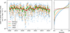 |
Figure 1 GOES-16 MPS-HI Omnidirectional Differential Electron Flux (FEDO) data from 2018 to 2024. Daily, weekly, monthly, and semi-annual averages are presented on the left plot. The corresponding cumulative distributions are presented on the right, with the mean flux level represented by the black dotted line. |
In this work, we model the instantaneous and averaged fluxes, at one location or averaged along a trajectory, as random variables. The distributions of these variables represent the possible observations of the fluxes on a long timescale.
For instantaneous fluxes, we can estimate their distributions, depending on the energy and location, either by binning in-situ observations or by using the empirical distributions from a reanalysis database. As the reanalysis database has limited resolution, some statistical modelling is required to produce a global, continuous estimation of the flux distributions. The spatial distribution model developed during this project is presented in Section 3.
The distribution of the average flux (or, equivalently, of the fluence) along a given trajectory can be obtained from the joint distribution of the instantaneous fluxes at the different points of the trajectory. Indeed, if we note Xi the random variable representing the flux at the ith point of the trajectory, the average flux can be represented by the variable
 (3)
(3)
where T is the total duration, and dti is the time passed around each trajectory point.
We note however that, in general, the Xi are not independent variables (actually, they are often highly correlated), which means that, to compute the distribution of the mean flux  , we need to know not only the distribution of each Xi independently, but also their complete joint probability distribution, which accounts for the correlation structure between all the different components.
To model such a dependency structure between random variables, and given that the fluxes distributions do not have a simple form in general (e.g., they are not Gaussian), a classical statistical approach is to introduce the copula of the distribution (Durante & Sempi, 2010). The copula C of a multivariate distribution (X1, …, Xn), with marginal cumulative distributions (CDF) Fi(xi) = Pr[Xi ≤ xi], is the joint distribution function:
![Mathematical equation: $$ C({u}_1={F}_1({X}_1),\dots,{u}_n={F}_n({X}_n))=\mathrm{Pr}[{F}_1({X}_1)\le {u}_1,\dots,{F}_n({X}_n)\le {u}_n]. $$](/articles/swsc/full_html/2025/01/swsc250019/swsc250019-eq6.gif) (4)
(4)
By normalizing each component by its CDF, we can decouple the specific characteristic of each component (which is represented by the corresponding marginal CDF), of the dependency structure between the components (which is represented by the copula). If we can model this copula for a given list of trajectory points, we can then sample the joint distribution and properly estimate the distribution of the mean flux or fluence along the trajectory. The covariance modelling performed in this project is presented in Section 5.
Modelling both the local flux distributions and the correlation structure allows us to produce a very powerful model. By sampling the joint probability, we obtain scenarios of possible flux observations along the spacecraft trajectory, which can then be analysed to produce the distributions of multiple quantities of interest:
the instantaneous flux distribution at each point of the trajectory (this is simply the local flux distribution at each point of the trajectory),
the cumulative fluence distribution along the trajectory,
the distributions of the mean flux on arbitrary periods (e.g., a few hours) along the trajectory.
The estimation of these distributions directly responds to the user’s need for environment specification, both for peak flux effects (such as charging) and for long-term average effects (such as dose). Moreover, a statistical sampling of the fluxes along the trajectory could also be directly fed to effect models, providing a probabilistic estimation of the corresponding risk.
4 Modelling local flux distributions
To model the global distributions of the fluxes, as presented above, we first need to build a model of the local distribution at each point in space and in energy. These local distributions correspond to the marginals of a joint distribution of the fluxes along the trajectory of the spacecraft and represent the local variability of the radiative environment.
In the literature, various analytical distribution functions have been used to model the observed flux distributions (O’Brien, 2005), including most notably the log-normal distribution (Brunet et al., 2021) and the Weibull distribution (Ginet et al., 2013). We can fit such analytical distribution functions on the fluxes from the GLORAB reanalysis database.
For simplicity, another numerical approach was used, which avoids the limitations of the analytical formula by just computing pairs of flux and probability values from the data points themselves and then uses interpolations in between these to estimate the flux values for a given probability of exceedance. Naturally, this method is incapable of producing estimates outside the limits of fluxes/probabilities that are already in the data, as it does not use an analytical form that can be used for that, so no extrapolations are possible. Thankfully, the number of data points that are in each grid point is enough to allow for estimates up to the 99th percentile for almost all points, so this is not as critical a drawback as it is for other applications of this method where fewer data are concerned.
5 A spatio-temporal covariance model for the particle fluxes
In this section, we present the development of a novel statistical model for the covariance of the fluxes along a spacecraft trajectory.
A large literature exists on statistical modelling of high dimensional copulas (Müller & Czado, 2019), and multiple families of copulas were introduced in the past, including most notably the Archimedean copulas (Nelsen, 1997), Vine copulas (Czado & Nagler, 2022), and Elliptical copulas (Frahm et al., 2003), which have different properties regarding their flexibility and tractability.
We note that often these copula models are fitted from a database of samples of the distribution of interest. However, in our case, the trajectory points are mission-dependent and only known during the runtime of the model, at which point we do not have access to the full reanalysis database to perform such fitting of the covariance functions.
The goal of the covariance model is to estimate, from the spatial and temporal coordinates of the points of the trajectory, the copula of the joint distribution of the fluxes at each point:
![Mathematical equation: $$ {Ec},\{{P}_i=({y}_i,{L}_i^{\mathrm{*}},{t}_i)|i\in [1,n]\}\to {C}_{{X}_1,\dots,{X}_n}. $$](/articles/swsc/full_html/2025/01/swsc250019/swsc250019-eq7.gif) (5)
(5)
5.1 Selection of a copula family
To select a modelling strategy, we first had to analyse the joint distributions between different points. Figure 2 presents, in the top row, the joint distributions between the 1 MeV normalized electron fluxes at various points of the Salammbô domain. We notice a wide range of regimes depending on the points considered, with densities highly clustered around the diagonal for points on the same L-shell (column on the right), slightly more spread out for points in the outer belt (middle column), and nearly uniform joint densities between the inner and outer belts (column on the left). We note that the statistical sampling in the inner belt is poorer than in the outer belt due to the greater characteristic timescales involved.
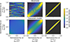 |
Figure 2 Joint distributions of the normalized 1MeV FEDO at L* = 5.7 and αeq = 86° and at different points of the domain (the coordinates of each point are presented at the bottom of each column). The top row shows the empirical joint probability distribution density, and the bottom row presents the corresponding probability density of a fitted Gaussian copula. |
We also note that there is no significant asymmetry in the joint distributions, which allows us to investigate the use of a Gaussian copula, which is defined as the copula function of a multivariate Gaussian distribution. This copula is a simple, elliptical, symmetric copula entirely determined by its correlation matrix R, with the following expression:
 (6)
(6)
where ΦR is the joint CDF of a multivariate normal distribution with zero mean and a correlation matrix equal to r, and Φ−1 is the inverse CDF of a standard normal distribution. Note that, while the Pearson correlation matrix Rij is usually used to parametrize the Gaussian copula, it can equivalently be parametrized by the Spearman rank correlation coefficients  , which corresponds to the Pearson correlation matrix of the normalized uniform variables, with the following correspondence formula (Kendall, 1949):
 (7)
(7)
In the following, we only deal with the normalized uniform variables, so all correlation coefficients will correspond to the Spearman correlation coefficients Rs.
This copula is presented in Figure 2, in the bottom row, with a correlation matrix R fitted on the reanalysis fluxes. Remarkably, we can see that the Gaussian copula is able to replicate the different regimes depending on the points coordinates, at least as a first-order approximation.
Hence, this justifies our choice to use a Gaussian copula model in this work. Our model, then has to estimate the correlation matrix R between the normalized fluxes at each point of the input trajectory. This significantly reduces the dimension of our problem, because each coefficient Rij of the correlation matrix only depends on the coordinates of two points of the trajectory and the temporal interval between them.
5.2 Temporal correlation model
Using the normalized fluxes obtained from the reanalysis database, we can study the variation of the correlation coefficient R as a function of the points’ coordinates, energy, and time interval. As one could expect, we have noticed an important and complex impact of the time interval on the correlation coefficient. Figure 3 presents, in blue, the evolution of the autocorrelation of the normalized electron fluxes at one point of the domain, as a function of the time interval. We note a strong variation of the R coefficient, with noticeable oscillations at different periods.
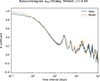 |
Figure 3 Autocorrelogram of the normalized equatorial electron fluxes at 566 keV and L* = 4.49, data from the reanalysis database (in blue) and fitted temporal model (in orange). |
We can physically explain the observed oscillations in the correlogram by space weather and space climate processes that affect the trapped particles’ fluxes:
the Solar Cycle (SC, Miyoshi & Kataoka, 2011) modulates the sun activity, and hence the radiation belt fluxes, with a periodicity of around 11 years,
the Semi-Annual Variation (SAV, Katsavrias et al., 2021), which corresponds to the evolution of the geomagnetic configuration as the Earth orbits the sun, and leads to a periodic variation of the geoeffectiveness of solar storms, with a periodicity of 6 months,
the effect of Corotating Interaction Regions (CIR, Hudson et al., 2008), which are linked to persistent coronal holes on the sun’s surface and periodically impact the Earth due to the apparent rotation of the surface of the sun, with a period of about 27 days. The coronal holes structures can persist from a few months to around one year on the sun surface (Bohlin, 1976), so we expect a decreasing impact on the correlograms with increasing time intervals, with no noticeable effects for time intervals above 1 year.
We note that the relative impact of each of these periodic components is highly dependent on the considered points locations and energies. For instance, fluxes in the outer radiation belt will be highly impacted by space weather effects (SAV and CIR), much more than the fluxes in the inner belt. Moreover, while the periods of these components are fixed, the phase of each component depends on the considered points too.
With this a priori knowledge of the dynamics of the radiation belts’ fluxes, we introduce the following temporal model Rθ:
 (8)
(8)
 (9)
(9)
 (10)
(10)
 (11)
(11)
 (12)
(12)
with θ = (R0, τstorm, τcir, αcir, Φcir, αsav, Φsav, αsc, Φsc) is the temporal model parameters, and ωsc = 11 years, ωsav = 0.5 years and ωcir = 27.27 days. This model, fitted to the data, is shown in orange in Figure 3. One can readily observe that the temporal dynamics of the correlation coefficient is properly captured by the model.
5.3 Correlation modelling
To model the correlation coefficient for an arbitrary pair of points using the temporal correlation presented above, we need to map from the points’ coordinates and time interval to the temporal parameters vector θ. Due to the dimension of the input space, the number of parameters of the temporal model, and the non-linear relationship between them, we have chosen a machine-learning approach to build this mapping. A large random sampling of pairs of points  in the domain was performed, and the corresponding temporal model parameters θ(Pi, Pj, Δt) were fitted on the correlograms obtained from the reanalysis database.
Several machine-learning models were compared. As a baseline for comparison, we have fitted a linear model. Then we have fitted a Gradient Boosting regressor (Bentéjac et al., 2021), using the Histogram-based implementation from the Scikit-Learn library (Pedregosa et al., 2011). Finally, we have defined and trained a neural network model (Marquez et al., 1991), using 3 dense hidden layers of size 512 with Rectified Linear Units (Zeiler et al., 2013) activation functions and dropout layers (LeCun et al., 2015). Each model was fitted using the same pre-computed sample database. In the case of the neural network, 10% of the points were randomly chosen for validation, and the remaining points were used for the training.
To compare the fitted models, we have selected representative points in L* and energy, and computed the correlation coefficients between them and every point in a grid in L*, equatorial pitch angle, and time interval. For each representative point, we have then computed the root-mean-square error (RMSE) between the R values computed from the reanalysis database and those predicted by the different models. The resulting RMSE values are presented in Table 1. We can see that, with the selected parameters, the Neural Network model significantly outperforms all other models.
Modelling error (RMSE) for the different models of correlation.
We note that, in the case of the Gradient Boosting model, we could increase the accuracy of the model by changing its parameters, at the cost of increased processing time during the fitting, but more crucially during the prediction at runtime. The results presented here correspond to a trade-off between the model error and the execution time of the model, which are already about 25 times slower than the Neural Network model. During the development, we did not find that a very large Gradient Boosting model would significantly outperform our Neural Network model, and that the processing time for such a model would be prohibitively large for the end-user model.
Figure 4 presents an overview of the correlation model results, compared to the observed correlation from the GLORAB reanalysis database. While some discrepancies can be observed locally, for instance near the loss-cone, or for very low L* values at low energy, we can see that the model is able to reproduce the various correlation structures at the different L* and energy values.
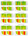 |
Figure 4 Observed and modelled correlation coefficient for normalized electron fluxes. Each group of four plots represents the correlation coefficient for the equatorial fluxes at a given L* and energy with all equatorial points at the same energy as a function of L* and time interval (top plots) and with all points at the same energy with no time interval as a function of L* and y (bottom plots). |
The residual neural network modelling RMSE ranges from 4% to 8%, depending on the considered L* value, according to Table 1. We note that it would be hard to predict how these errors would affect the final flux predictions on a given trajectory, which spans different L* and y values. While more resources could be dedicated to improve the model precision, for instance by sampling more data points, or increasing the model complexity, we believe the model outputs are precise enough, given the comparatively large uncertainties in the input reanalysis database used in this study.
6 Specifying the radiation belt environment for a spacecraft mission
Here we present the architecture of the GLORAB radiation belt specification model, which uses the statistical model presented above to estimate the distributions of the instantaneous fluxes and the cumulative fluences along a given spacecraft trajectory.
The GLORAB model uses a two-pass method to compute the flux distributions for a wide range of missions.
The first pass takes the user-supplied trajectory of the mission and produces samples of instantaneous fluxes scenarios along this trajectory, using the correlation and distribution models presented above.
The second pass, which is optional, allows to estimate the evolution of the fluxes when the input trajectory segment is repeated a number of times. This can be used for long missions for which the trajectory is highly repetitive, and provides an estimation of the mean flux for each trajectory segment along the full mission duration.
From the sampled fluxes (along the trajectory and for different trajectory repetitions), we can compute the cumulative fluence distribution or the average fluxes on different time intervals.
6.1 Input user trajectory
The trajectory is provided as a SPENVIS (Heynderickx et al., 2004) trajectory file, which contains the geographic coordinates of the trajectory points and the time epoch.
From these geographic coordinates, we compute the magnetic coordinates (y, L*) with the Olson-Pfitzer Quiet magnetic field model (Olson & Pfitzer, 1974), using the IRBEM library (Boscher et al., 2022).
6.2 First pass – estimating flux distributions along the trajectory
During the first pass, we produce samples of the flux along the trajectory. Each sample corresponds to a possible flux evolution at the different points of the trajectory.
The model constructs the correlation matrix of the normalized fluxes at the different points by evaluating the correlation model presented in Section 5 for each pair of trajectory points. This correlation matrix is then factorized using an Eigenvalue Decomposition (Dietrich & Newsam, 1997):
 (13)
(13)
where Q is a square matrix composed of the eigenvectors of R, and Λ is a diagonal matrix containing the corresponding eigenvalues. We note that the eigenvalue decomposition has this form because R is real and symmetric. As R is a correlation matrix, it should be positive semi-definite and the eigenvalues should all be non-negative. However, as this property is not strictly enforced in the correlation model, in practice, we observe some slightly negative eigenvalues, which we truncate to zero. We build the square root matrix
 (14)
(14)
where  is the diagonal matrix containing the square root of the eigenvalue, so we have
 (15)
(15)
Then, if X is a random vector of size N, the number of trajectory points, with multivariate normal distribution with zero mean and identity covariance matrix, HX is a normally-distributed random vector with zero mean and correlation matrix HINHT = R. Hence, we can randomly sample a vector with independent normal components and, by multiplying by the H matrix, obtain a sample of a multivariate normal distribution with a correlation matrix of R. We can then compute the sampled normalized fluxes ui by applying to each component the CDF of the normal distribution.
The flux samples xi are then produced by applying the inverse CDF  , presented in Section 4 at each point of the trajectory to the normalized fluxes:
 (16)
(16)
This sampling is performed a large number of times, producing an ensemble of flux samples along the trajectory. In the following, we use the superscript to denote the index of a sample in the ensemble, so that  represents the sampled flux at the ith trajectory point for the kth ensemble member.
6.3 Second pass – estimating mean flux distributions for trajectory repetitions
When the spacecraft trajectory is highly repetitive, which is the case for most missions, we would like to know the radiation environment for the complete mission without sampling the full trajectory. Indeed, precisely sampling the trajectory for very long repetition would unnecessarily require a huge number of trajectory points, and modelling its radiation environment could quickly become intractable. For these missions, as is typical for specification models, the user should only provide one period of the trajectory, and somehow specify the total mission duration. Here we note that one period of the trajectory should be understood in magnetic coordinates, and often corresponds to multiple orbit revolutions, due to longitudinal effects.
In our model, the user can provide the number of period repetitions to model, and it will produce samples of the mean flux for each period repetition of the input trajectory segment. To do this, we need to estimate the marginal distribution of the mean flux during one trajectory segment, as well as the temporal covariance between the mean fluxes during different segment repetitions.
The marginal distribution of the mean flux during one trajectory segment can be estimated empirically from the ensemble of instantaneous flux samples produced during the first pass. For each sample, we can compute the average flux
 (17)
(17)
yielding the empirical distribution of the flux averaged over one trajectory period.
To estimate the temporal covariance between the fluxes at different trajectory repetitions, we will use the temporal correlation model presented in Section 5, evaluated at a representative trajectory point. To identify this representative point, we compute the correlation between the fluxes at each trajectory point with the average flux, and select the point i* at which this correlation is maximum:
 (18)
(18)
where the correlation is taken along the k members of the sampled ensemble.
We expect the flux at this representative point to be highly correlated to the average flux, and to have a temporal auto-correlation function very close to that one of the average flux.
Using the correlation model presented in Section 5, we compute this auto-correlation function R(Δt), and construct the correlation matrix of the normalized mean flux at the different trajectory period repetitions. As the time interval between successive repetitions is constant, the obtained correlation matrix has a very particular structure, where each diagonal is constant. This type of matrix is called a Toeplitz matrix (Gray, 2006) in the literature. This particularity means that we do not need to actually construct the full matrix, as its first row or column is a sufficient, space efficient representation. To sample the distribution represented by this correlation matrix, we could perform a factorization as before, but this factorization would not have a sparse representation. A common technique to perform the sampling of such a distribution (often called a stationary Gaussian process) is to embed the Toeplitz correlation matrix in a larger so-called circulant matrix, which can be sampled efficiently using a Fast Fourier Transform (Dietrich & Newsam, 1997). As before, the sampled points are normalized using the CDF of the unit normal distribution to obtain the sampled normalized fluxes. The latter are then used to compute the mean flux for each trajectory repetition by applying the empirical inverse CDF of the average flux distribution.
6.4 Model outputs
From the sampled ensemble of fluxes along the trajectory and mean fluxes along the trajectory repetitions, the model then evaluates any quantile levels of the instantaneous flux distributions along the trajectory and of the cumulative fluence distributions across the different orbit repetitions.
As examples, Figure 5 presents the summary plots obtained with the electron model for the orbit of the Arase (Miyoshi et al., 2017). For this plot, one orbit revolution was used as input trajectory, and we have set a number of trajectory repetitions to reach around 10 years of mission.
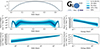 |
Figure 5 GLORAB model results overview for the Arase orbit. The top panel presents the L* coordinate of the satellite along its orbit. The left panels present the predicted distributions at 380 keV for the instantaneous fluxes along the trajectory (at the centre) and the cumulative distributions along the mission (at the bottom). The panels on the right present the mean orbital (at the centre) and total mission fluence (at the bottom) distributions as a function of the energy. |
We can observe, on the instantaneous flux plot at 380 keV, both the inner and outer radiation belts, once on the ascending and once on the descending parts of the orbit. At this energy, we notice the large spread in the fluxes, for L* values above 2. The mean orbital flux spectrum plot on the right shows that the variance is relatively uniform in energy. The bottom plot presents the cumulative fluence at 380 keV along the mission. We notice that the distribution progressively narrows down to a mean, and that this progression is not uniform in time. We see in particular a steeper decrease in the variance between 1000 and 3000 days, which is due to the effect of the solar cycle. Comparing the total mission fluence spectrum plot at the bottom right of Figure 5 with the mean orbital flux spectrum plot, we notice this effective shrinking of the distribution, which is due to the averaging on the long mission duration.
This example highlights the usefulness of the model and its capability to give a much more detailed overview of the expected radiation environment for a given mission profile, compared to traditional models. Indeed, this model not only provides long-term average spectrum, but also depicts its dynamics at all timeframes.
7 Model results and comparison
The only other publicly available specification model which provides a similarly detailed specification of the radiation environment is the IRENE model (Ginet et al., 2013), using its Monte-Carlo mode. Hence, in this section, we will compare our model with AE9 (the energetic electron component of IRENE).
We illustrate the model predictions on the orbit of the American GPS satellite Navstar 54 (NS54), since we have approximately 20 years of electron flux observation by the Combined X-ray and Dosimeter (CXD2R, Morley et al., 2017) instrument onboard. This instrument provides 15 channels of differential electron flux measurements, from 120 keV to 10 MeV.
As input trajectory, we have used 10 days of the satellite trajectory, which corresponds to 20 orbit revolutions, sampled at a period of 30 min – thus consisting of 480 trajectory points. This 10 days trajectory segment was then repeated 401 times to construct an 11 years mission. In our model this number of repetition is one of the model parameters. For AE9, the segment was simply repeated in the input trajectory, giving 192,480 trajectory points.
As mentioned above, the AE9 model was used in Monte-Carlo mode, using 200 members. IRENE version 1.58.001 was used. The total computing time was around 120 s for the GLORAB model and around 12 h for the AE9 model.
Figure 6 presents an overview of the obtained spectra, compared to the CXD2R observations. The solid lines present for each dataset the median long-term (11 years) mean flux. It is apparent that there is a large disagreement between the two models and with the data, albeit this disagreement is not the same at all energies.
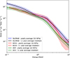 |
Figure 6 Yearly averages distribution and median 11-year average for the electron fluxes along the NS54 trajectory. The blue curves present our model results, the red curves the CXD2R observations, and the green curves the AE9 results. |
At low (<300 keV) and very high (>2.5 MeV) energies, our model slightly over-predicts the fluxes compared to both the AE9 prediction and the observation, which can be explained by the physical limitations of the underlying 3D drift-averaged Salammbô model (Dahmen et al., 2025). At low energies, the AE9 gives an excellent prediction for the fluxes, which closely matches the NS54 observations, both in terms of long-term average and for the distribution of yearly averages. Similarly, at very high energies, the AE9 prediction seems to match the observations, although the predicted spread in the yearly averages is significantly smaller than observed. Generally, concerning the spread of the yearly average distributions, both models predict similar spreads, which are nearly constant across all energies.
Around 1 MeV, however, our model shows close agreement with the NS54 observations. This is expected because the GPS data was assimilated during the construction of the database in this energy range. On this energy range, the AE9 prediction of the flux is significantly lower.
One of the key features of our model is its capability to predict the cumulative fluence distribution along the spacecraft mission. This is illustrated in Figure 7, which presents the predicted and observed cumulative 2 MeV fluence distributions for the NS54 satellite over a duration of 10 years. In Figure 7, the panel on the left shows the raw data, from both our model (in blue) and AE9 (in green). The red curves show the cumulative fluence distribution observed by CXD2R, by integrating the fluxes over the given duration and from varying start dates in the dataset.
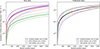 |
Figure 7 Cumulative fluences along the NS54 mission. The left panel shows the raw datasets (our model in blue, NS54/CXD2R data in red, AE9 in green). The right panel shows the same fluence with both models calibrated to have the same median long-term average as the observation data. In each plot, the thick solid lines present the median values and the dashed lines present the 10th and 90th percentiles. |
It can be seen that our model is able to produce a good reconstruction of the observed fluence distributions along the mission duration. However, it is hard to compare the two models and the observation data using Figure 7, because of the important bias between their long-term means. To compensate for this bias, we have calibrated both models so that their long-term (11 years) averages match the one from the observation. The resulting fluences are presented in Figure 7 on the right panel.
When using calibrated models, it is apparent that both our model and the AE9 model can reproduce the dynamics of the median of the fluence distribution along time. Concerning the spread of this distribution, as represented by the 10th and 90th percentiles in Figure 7, our model follows more closely the evolution observed in the data, with a much steeper narrowing of the distribution from 1000 to 3500 days of mission duration, compared to AE9 which has a nearly constant relative variance at all times.
8 Conclusion
In this paper, we presented the construction of a statistical model extracted from the GLORAB reanalysis database introduced in Dahmen et al. (2025). This model was used as the core of the GLORAB prototype specification model of the radiation environment.
By using a statistical model that not only describes the distribution of the energetic particles fluxes in space, but also how they correlate in space and time, we were able to build a very powerful specification model. Indeed, the GLORAB model can produce, for a given space mission profile, not only the instantaneous flux distributions, but also the cumulative fluences along the mission for any required mission duration. We believe this novel approach can help spacecraft designers to better take into account the natural variability of the trapped radiation environment. While powerful, our model remains fast to run (with complex missions taking from a few seconds to a few minutes to compute), and easy to use for all radiation models users. In particular, it is much faster than the IRENE framework in Monte-Carlo mode, which provides comparable outputs.
The main limitation of this approach is its dependence on a good-quality reanalysis database. Contrary to the IRENE models, which incorporate a very extensive database of radiation belt observations, our method relies on the availability of full PSD maps, which can only be produced using data assimilation and modelling. As was presented here, the GLORAB reanalysis database time range is quite limited (mainly to the Van Allen Probes era and later), and does show some bias, especially at low energies or high L* values. In future works, we expect that new developments in both the physical modelling of the radiation belts and in data assimilation methods will allow the community to produce better and longer reanalysis databases, which would allow us to improve the GLORAB specification model.
Acknowledgments
The authors gratefully acknowledge the CXD team at Los Alamos National Laboratory for the use of the GPS CXD data and NOAA for the use of the GOES-16 MPS-HI data. The editor thanks two anonymous reviewers for their assistance in evaluating this paper.
Funding
This work received funding from the European Space Agency under ESA Contract 4000137689/22/NL/CRS.
Data availability statement
Data access to the GPS-NS54 and GPS-NS72 CXD electron fluxes is provided by the NOAA Solar and Terrestrial Physics Branch (https://www.ncei.noaa.gov/products/space-weather/partners/lanl-products-data).
The GOES-16/MPS-HI particle data were produced by the NOAA Space Weather Prediction Center (SWPC) and are distributed by the NOAA National Centers for Environmental Information (NOAA-NCEI, https://data.ngdc.noaa.gov/platforms/solar-space-observing-satellites/goes/goes16/l2/data/mpsh-l2-avg1m_science/).
References
- Bentéjac C, Csörgő A, Martínez-Muñoz G. 2021. A comparative analysis of gradient boosting algorithms. Artif Intell Rev 54(3): 1937–1967. https://doi.org/10.1007/s10462-020-09896-5. [Google Scholar]
- Bohlin J. 1976. The physical properties of coronal holes. In: Physics of Solar Planetary Environments: Proceedings of the International Symposium on Solar-Terrestrial Physics, June 7–18, Boulder, Colorado, vol. I, American Geophysical Union (AGU), pp. 114–128. ISBN 978-1-118-66904-4. https://doi.org/10.1029/SP007p0114. [Google Scholar]
- Boscher D, Bourdarie S, O’Brien P, Guild T, Heynderickx D, et al. 2022.PRBEM/IRBEM: V5.0.0. Zenodo. Available at https://doi.org/10.5281/zenodo.6867768. [Google Scholar]
- Boscher D, Sicard-Piet A, Lazaro D, Cayton T, Rolland G. 2014. A new proton model for low altitude high energy specification. IEEE Trans Nucl Sci 61(6): 3401–3407. https://doi.org/10.1109/TNS.2014.2365214. [CrossRef] [Google Scholar]
- Bourdarie S, Blake B, Cao JB, Friedel R, Miyoshi Y, Panasyuk M, Underwood C. 2012. Standard file format guidelines for particle fluxes, Technical Report V1.2, COSPAR Panel on Radiation Belt Environment Modeling (PRBEM). Available at https://prbem.github.io/documents/Standard_File_Format.pdf. [Google Scholar]
- Brunet A, Sicard A, Papadimitriou C, Lazaro D, Caron P. 2021. OMEP-EOR: a MeV proton flux specification model for electric orbit raising missions. J Space Weather Space Clim 11: 55. https://doi.org/10.1051/swsc/2021038. [Google Scholar]
- Czado C, Nagler T. 2022. Vine copula based modeling. Ann Rev Stat Appl 9: 453–477. https://doi.org/10.1146/annurev-statistics-040220-101153. [Google Scholar]
- Dahmen N, Papadimitriou C, Brunet A, Sicard A, Aminalragia-Giamini S, Sandberg I. 2025. Robust reanalysis of the electron radiation belt dynamics for physics driven space climatology applications. J Space Weather Space Clim 15: 13. https://doi.org/10.1051/swsc/2025009. [Google Scholar]
- Dietrich CR, Newsam GN. 1997. Fast and exact simulation of stationary gaussian processes through circulant embedding of the covariance matrix. SIAM J Sci Comput 18(4): 1088–1107. https://doi.org/10.1137/S1064827592240555. [Google Scholar]
- Durante F, Sempi C. 2010. Copula theory: an introduction. In: Copula theory and its applications, Jaworski P, Durante F, Härdle WK, Rychlik T (Eds.), Springer, Berlin, Heidelberg, pp. 3–31. ISBN 978-3-642-12465-5. https://doi.org/10.1007/978-3-642-12465-5_1. [Google Scholar]
- Frahm G, Junker M, Szimayer A. 2003. Elliptical copulas: applicability and limitations. Stat Probab Lett 63(3): 275–286. https://doi.org/10.1016/S0167-7152(03)00092-0. [Google Scholar]
- Galica GE, Dichter BK, Tsui S, Golightly MJ, Lopate C, Connell JJ. 2016. GOES-R space environment in-situ suite: instruments overview, calibration results, and data processing algorithms, and expected on-orbit performance. In: Earth Observing Missions and Sensors: Development, Implementation, and Characterization IV, vol. 9881, SPIE, pp. 237–251. https://doi.org/10.1117/12.2228537. [Google Scholar]
- Ginet GP, O’Brien TP, Huston SL, Johnston WR, Guild TB, et al. 2013. AE9, AP9 and SPM: new models for specifying the trapped energetic particle and space plasma environment. Space Sci Rev 179(1): 579–615. https://doi.org/10.1007/s11214-013-9964-y. [CrossRef] [Google Scholar]
- Gray RM. 2006. Toeplitz and circulant matrices: a review. Found Trends Commun Inf Theory 2(3): 155–239. https://doi.org/10.1561/0100000006. [Google Scholar]
- Heynderickx D, Quaghebeur B, Wera J, Daly EJ, Evans HDR. 2004. New radiation environment and effects models in the European Space Agency’s Space Environment Information System (SPENVIS). Space Weather 2(10): S10S03. https://doi.org/10.1029/2004SW000073. [Google Scholar]
- Hudson MK, Kress BT, Mueller H-R, Zastrow JA, Bernard Blake J. 2008. Relationship of the Van Allen radiation belts to solar wind drivers. J Atmos Sol Terr Phys 70(5): 708–729. https://doi.org/10.1016/j.jastp.2007.11.003. [Google Scholar]
- Katsavrias C, Papadimitriou C, Aminalragia-Giamini S, Daglis IA, Sandberg I, Jiggens P. 2021. On the semi-annual variation of relativistic electrons in the outer radiation belt. Ann Geophys 39(3): 413–425. https://doi.org/10.5194/angeo-39-413-2021. [Google Scholar]
- Kendall MG. 1949. Rank and product-moment correlation. Biometrika 36(1/2): 177–193. https://doi.org/10.2307/2332540. [Google Scholar]
- Kwan BP, O’Brien TP. 2015. Using static percentiles of AE9/AP9 to approximate dynamic monte carlo runs for radiation analysis of spiral transfer orbits. IEEE Trans Nucl Sci 62(3): 1357–1361. https://doi.org/10.1109/TNS.2015.2423235. [Google Scholar]
- LeCun Y, Bengio Y, Hinton G. 2015. Deep learning. Nature 521(7553): 436–444. https://doi.org/10.1038/nature14539. [Google Scholar]
- Marquez L, Hill T, Worthley R, Remus W. 1991. Neural network models as an alternative to regression. In: Proceedings of the Twenty-Fourth Annual Hawaii International Conference on System Sciences, vol. 4, Kauai, HI, USA, 08–11 January, pp. 129–135. https://doi.org/10.1109/HICSS.1991.184052. [Google Scholar]
- Miyoshi Y, Kasaba Y, Shinohara I, Takashima T, Asamura K, et al. 2017. Geospace exploration project: arase (ERG). J Phys Conf Ser 869(1): 012095. https://doi.org/10.1088/1742-6596/869/1/012095. [Google Scholar]
- Miyoshi Y, Kataoka R. 2011. Solar cycle variations of outer radiation belt and its relationship to solar wind structure dependences. J Atmos Sol Terr Phys 73(1): 77–87. https://doi.org/10.1016/j.jastp.2010.09.031. [Google Scholar]
- Morley SK, Sullivan JP, Carver MR, Kippen RM, Friedel RHW, Reeves GD, Henderson MG. 2017. Energetic particle data from the global positioning system constellation. Space Weather 15(2): 283–289. https://doi.org/10.1002/2017SW001604. [CrossRef] [Google Scholar]
- Müller D, Czado C. 2019. Dependence modelling in ultra high dimensions with vine copulas and the graphical lasso. Comput Stat Data Anal 137: 211–232. https://doi.org/10.1016/j.csda.2019.02.007. [Google Scholar]
- Nelsen RB. 1997. Dependence and order in families of archimedean copulas. J Multivariate Anal 60(1): 111–122. https://doi.org/10.1006/jmva.1996.1646. [Google Scholar]
- O’Brien TP. 2005. A framework for next-generation radiation belt models. Space Weather 3(7): S07B02. https://doi.org/10.1029/2005SW000151. [Google Scholar]
- O’Brien TP, Johnston WR, Huston SL, Roth CJ, Guild TB, Su Y-J, Quinn RA. 2018. Changes in AE9/AP9-IRENE version 1.5. IEEE Trans Nucl Sci 65(1): 462–466. https://doi.org/10.1109/TNS.2017.2771324. [CrossRef] [Google Scholar]
- Olson WP, Pfitzer KA. 1974. A quantitative model of the magnetospheric magnetic field. J Geophys Res 79(25): 3739–3748. https://doi.org/10.1029/JA079i025p03739. [Google Scholar]
- Pedregosa F, Varoquaux G, Gramfort A, Michel V, Thirion B, et al. 2011. Scikit-learn: machine learning in Python. J Mach Learn Res 12(85): 2825–2830. http://jmlr.org/papers/v12/pedregosa11a.html. [Google Scholar]
- Sawyer DM, Vette JI. 1976. AP-8 trapped proton environment for solar maximum and solar minimum, Technical Report NSSDC/WDC-A-R/S-76-06. Available at https://ntrs.nasa.gov/citations/19770012039. [Google Scholar]
- Sicard A, Boscher D, Bourdarie S, Lazaro D, Standarovski D, Ecoffet R. 2018. GREEN: the new global radiation earth environment model (beta version). Ann Geophys 36(4): 953–967. https://doi.org/10.5194/angeo-36-953-2018. [Google Scholar]
- Sicard-Piet A, Bourdarie S, Boscher D, Friedel RHW, Thomsen M, Goka T, Matsumoto H, Koshiishi H. 2008. A new international geostationary electron model: IGE-2006, from 1 keV to 5.2 MeV. Space Weather 6(7): S07003. https://doi.org/10.1029/2007SW000368. [CrossRef] [Google Scholar]
- Vette JI. 1991. The AE-8 trapped electron model environment. Technical Report NSSDC/WDC-A-RS-91-24, National Space Science Data Center (NSSDC), World Data Center A for Rockets and Satellites. Available at https://ntrs.nasa.gov/citations/19920014985. [Google Scholar]
- Zeiler M, Ranzato M, Monga R, Mao M, Yang K, et al. 2013. On rectified linear units for speech processing. In 2013 IEEE International Conference on Acoustics, Speech and Signal Processing, Vancouver, BC, Canada, 26-31 May IEEE, pp. 3517–3521. https://doi.org/10.1109/ICASSP.2013.6638312. [Google Scholar]
All Tables
All Figures
|
Figure 1 GOES-16 MPS-HI Omnidirectional Differential Electron Flux (FEDO) data from 2018 to 2024. Daily, weekly, monthly, and semi-annual averages are presented on the left plot. The corresponding cumulative distributions are presented on the right, with the mean flux level represented by the black dotted line. |
| In the text | |
|
Figure 2 Joint distributions of the normalized 1MeV FEDO at L* = 5.7 and αeq = 86° and at different points of the domain (the coordinates of each point are presented at the bottom of each column). The top row shows the empirical joint probability distribution density, and the bottom row presents the corresponding probability density of a fitted Gaussian copula. |
| In the text | |
|
Figure 3 Autocorrelogram of the normalized equatorial electron fluxes at 566 keV and L* = 4.49, data from the reanalysis database (in blue) and fitted temporal model (in orange). |
| In the text | |
|
Figure 4 Observed and modelled correlation coefficient for normalized electron fluxes. Each group of four plots represents the correlation coefficient for the equatorial fluxes at a given L* and energy with all equatorial points at the same energy as a function of L* and time interval (top plots) and with all points at the same energy with no time interval as a function of L* and y (bottom plots). |
| In the text | |
|
Figure 5 GLORAB model results overview for the Arase orbit. The top panel presents the L* coordinate of the satellite along its orbit. The left panels present the predicted distributions at 380 keV for the instantaneous fluxes along the trajectory (at the centre) and the cumulative distributions along the mission (at the bottom). The panels on the right present the mean orbital (at the centre) and total mission fluence (at the bottom) distributions as a function of the energy. |
| In the text | |
|
Figure 6 Yearly averages distribution and median 11-year average for the electron fluxes along the NS54 trajectory. The blue curves present our model results, the red curves the CXD2R observations, and the green curves the AE9 results. |
| In the text | |
|
Figure 7 Cumulative fluences along the NS54 mission. The left panel shows the raw datasets (our model in blue, NS54/CXD2R data in red, AE9 in green). The right panel shows the same fluence with both models calibrated to have the same median long-term average as the observation data. In each plot, the thick solid lines present the median values and the dashed lines present the 10th and 90th percentiles. |
| In the text | |
Current usage metrics show cumulative count of Article Views (full-text article views including HTML views, PDF and ePub downloads, according to the available data) and Abstracts Views on Vision4Press platform.
Data correspond to usage on the plateform after 2015. The current usage metrics is available 48-96 hours after online publication and is updated daily on week days.
Initial download of the metrics may take a while.