| Issue |
J. Space Weather Space Clim.
Volume 14, 2024
Topical Issue - CMEs, ICMEs, SEPs: Observational, Modelling, and Forecasting Advances
|
|
|---|---|---|
| Article Number | 1 | |
| Number of page(s) | 15 | |
| Section | Research Article | |
| DOI | https://doi.org/10.1051/swsc/2023032 | |
| Published online | 02 February 2024 | |
A Bayesian approach to the drag-based modelling of ICMEs
1
SP2RC, School of Mathematics and Statistics, University of Sheffield, Hicks Building, Broomhall, Sheffield S3 7RH, UK
2
Department of Physics, University of Rome “Tor Vergata”, Via della Ricerca Scientifica 1, Rome I-00133, Italy
3
IA, Instituto De Astrofisica E Ciências Do Espaço, University of Coimbra, Coimbra 3004-531, Portugal
4
Univ Lyon, CNRS, École Centrale de Lyon, INSA Lyon, Univ Claude Bernard Lyon I, LMFA UMR 5509, Ecully cedex F-69134, France
5
Dipartimento di Scienze Fisiche e Chimiche, Università dell’Aquila, Via Vetoio, L’Aquila 67100, Italy
6
Space Weather Research Technology Education Center (SWx-TREC), University of Colorado, Boulder, CO 80309, USA
7
Queen Mary University of London, London E1 4NS, UK
8
Department of Physics, Sapienza University of Rome, Piazzale Aldo Moro 5, Rome 00185, Italy
9
Department of Astronomy, Eötvös Loránd University, Pázmány Péter sétány 1/A, Budapest H-1112, Hungary
10
Hungarian Solar Physics Foundation, Petőfi tér 3, Gyula H-5700, Hungary
* Corresponding author: This email address is being protected from spambots. You need JavaScript enabled to view it.
Received:
23
August
2023
Accepted:
29
November
2023
Abstract
Coronal Mass Ejections (CMEs) are huge clouds of magnetised plasma expelled from the solar corona that can travel towards the Earth and cause significant space weather effects. The Drag-Based Model (DBM) describes the propagation of CMEs in an ambient solar wind as analogous to an aerodynamic drag. The drag-based approximation is popular because it is a simple analytical model that depends only on two parameters, the drag parameter  and the solar wind speed
  . DBM thus allows us to obtain reliable estimates of CME transit time at low computational cost. Previous works proposed a probabilistic version of DBM, the Probabilistic Drag Based Model (P-DBM), which enables the evaluation of the uncertainties associated with the predictions. In this work, we infer the “a-posteriori” probability distribution functions (PDFs) of the
  and
and  parameters of the DBM by exploiting a well-established Bayesian inference technique: the Monte Carlo Markov Chains (MCMC) method. By utilizing this Bayesian method through two different approaches, an ensemble and an individual approach, we obtain specific DBM parameter PDFs for two ensembles of CMEs: those travelling with fast and slow solar wind, respectively. Subsequently, we assess the operational applicability of the model by forecasting the arrival time of CMEs. While the ensemble approach displays notable limitations, the individual approach yields promising results, demonstrating competitive performances compared to the current state-of-the-art, with a Mean Absolute Error (MAE) of 9.86 ± 4.07 h achieved in the best-case scenario.
Key words: Coronal Mass Ejections / Drag Based Model / Space weather
© S. Chierichini et al., Published by EDP Sciences 2024
 This is an Open Access article distributed under the terms of the Creative Commons Attribution License (https://creativecommons.org/licenses/by/4.0), which permits unrestricted use, distribution, and reproduction in any medium, provided the original work is properly cited.
1. Introduction
Coronal Mass Ejections (CMEs) are the primary eruptive phenomena originating in the solar atmosphere and are known to cause severe space weather effects. The passage of their interplanetary counterparts (ICMEs) can lead to significant variations in near-Earth space solar wind conditions, posing a threat to space- and ground-based technologies (Schwenn, 2006; Pulkkinen, 2007; Temmer, 2021). Obtaining reliable predictions of the Time of Arrival (ToA) and Velocity of Arrival (VoA) of CMEs is a challenging task. Various limitations, including physical, observational, and modelling factors, hinder the effectiveness of existing CME forecasting methods (Vourlidas et al., 2019). In the past two decades, extensive efforts have been made to model CMEs and forecast their arrival on Earth. Established approaches initially included fully magnetohydrodynamic (MHD) models such as the WSA-ENLIL and EUFHORIA models (Odstrcil, 2003; Pomoell & Poedts, 2018). Although these methods proved reasonably efficient in providing arrival time prediction of CMEs, they are typically computationally intensive. However, more recently, with the advent of Artificial Intelligence (AI), forecasting tools based on Machine Learning (ML) methods have proved to be also effective using e.g. deep learning, and logistic regression ML. (Huang et al., 2018; Camporeale, 2019; Korsós et al., 2021). ML methods offer the advantage of providing timely predictions once the models have been trained; see e.g. the CME Arrival Time Prediction Using Machine learning Algorithms (CAT-PUMA) tool (Liu et al., 2018) or using convolutional neural network (CNN) approaches (Wang et al., 2019). Additionally, a category of (M)HD-based models has emerged, leveraging the hypothesis that the dynamics of CMEs in interplanetary space are governed exclusively by their interaction with the ambient solar wind (Cargill, 2004; Owens & Cargill, 2004; Shi et al., 2015). One popular model in this category is the Drag-Based Model (DBM) (Vršnak et al., 2013; Cargill, 2004; Napoletano et al., 2018; Dumbović et al., 2018). The DBM provides a simplified description of CME propagation dynamics in the solar wind, leveraging a description analogous to an aerodynamic drag due to the interplanetary medium. The DBM assumes that beyond a certain distance from the Sun (approximately 20 solar radii), ICMEs tend to adjust their velocity to match the interplanetary medium, with fast ICMEs decelerating and slow ICMEs tending to accelerate (Gopalswamy et al., 2000). However, despite of all the efforts, the accuracy of ToA predictions is still impacted by the limitations of available data. These limitations arise from the challenges of assessing CME properties at launch from remote sensing observations and the inability to accurately characterize the inner heliosphere. In a previous study, Napoletano et al. (2018), hereafter referred to as N1, introduced a probabilistic version of the DBM, the Probabilistic-DBM (P-DBM), to address the lack of information and provide estimates of the inherent uncertainty in CME forecasts. The P-DBM method upgrades the constant values of the DBM parameters with a-priori probability distributions (PDFs). In this way, it exploits the ensemble model approach to provide PDFs of ToA and VoA at a target location. This framework enables the generation of the most probable estimates of ToA and VoA, along with the associated prediction uncertainty (e.g. Del Moro et al., 2019; Piersanti et al., 2020). In a subsequent study, Napoletano et al. (2022) proposed a modified version of these PDFs employing an inversion procedure of DBM equations based on a Monte Carlo-like N1 and N2 explore the possibility that the PDF of the DBM parameters may differ depending on the type of solar wind accompanying the propagation of the CMEs. The dynamics of CMEs are modelled as that of a solid body moving in a fluid stream, suggesting that an appropriate description of the propagation dynamics is required for accelerated or decelerated CMEs. On average, they improved the knowledge of the parameters PDFs leading to a better prediction of the ToA. In this paper, we re-visit the P-DBM and propose to further improve the P-DBM by leveraging a popular Bayesian inference technique, the Monte Carlo Markov Chains (MCMC). MCMC algorithms are a class of Monte Carlo techniques that allow for the simulation of unknown distributions and open the way for their application to new problems (Brooks, 1998; Brooks et al., 2011). By utilizing MCMC methods, it is possible to numerically map a-posteriori distributions, even in highly complex frameworks involving high-dimensional parameter spaces and complex posterior structures with multiple peaks. We propose an update to the P-DBM parameter PDFs by harnessing the power of the Metropolis-Hastings MCMC algorithm and studying the application of these PDFs in the prediction of CME arrival time. Section 2 provides a description of the methods employed in this analysis, presenting a brief description of the DBM, emphasizing the features of the probabilistic version and outlining the main characteristics of MCMC methods. In Section 3 we introduce the dataset employed for the analysis. Finally, Sections 4 and 5 describe and discuss the results obtained.
2 Methods
2.1 The Drag-Based Model
The Drag-Based Model (Cargill, 2004; Vršnak et al., 2013) is a simplified kinematic model used to describe the propagation of CMEs in the interplanetary medium, the solar wind. The DBM framework assumes that the CMEs propagation is primarily influenced by a hydrodynamic-like drag force resulting from the interaction with the ambient solar wind. In this framework, the radial acceleration of a CME is determined by the solar wind speed w(r) and the drag parameter γ(r), following the equation:
![Mathematical equation: $$ a=-\gamma (r)[(v-w(r))]|v-w(r)|, $$](/articles/swsc/full_html/2024/01/swsc230044/swsc230044-eq5.gif) (1)
(1)
where v represents the CME velocity and r is the distance from the Sun. The drag parameter γ encapsulates information about the interaction between ICMEs and the solar wind and can be expressed as a function of the ICME cross-sectional area (A), the solar wind density (ρw), the ICME mass (M), and the virtual mass ( , where V is the ICME volume) (Cargill, 2004). It is typically expressed as:
 (2)
(2)
where cd is the drag coefficient. In general, the drag parameter γ may vary with time, but it is reasonable to assume that γ(r) and w(r) remain constant beyond approximately 20 solar radii (Cargill, 2004; Vršnak et al., 2013). Under this assumption, one can obtain the CME velocity v(t) and the heliospheric distance r(t) as functions of time:
 (3)
(3)
![Mathematical equation: $$ r(t)=\pm \frac{1}{\gamma }\mathrm{ln}[1\pm \gamma ({v}_0-w)t]+{wt}+{r}_0, $$](/articles/swsc/full_html/2024/01/swsc230044/swsc230044-eq9.gif) (4)
(4)
where v0 represents the initial CME velocity, and r0 is the initial heliospheric distance. The DBM framework allows us to make predictions for the ToA and the impact velocity (VoA) of a CME by fixing the travelled distance ( ) and using the DBM parameters as inputs. In N1, a probabilistic version of the DBM was introduced, referred to as P-DBM, which employs a-priori distributions of γ and w to obtain estimates of ToA and VoA along with their associated errors. In N1, the drag parameter γ is modelled using a log-normal probability distribution function (PDF) with mean μ = −0.70 and standard deviation σ = 1.01. The solar wind speed
  is modelled using a Gaussian PDF. Additionally, a distinction is made between decelerated CMEs (associated with slow solar wind) and accelerated CMEs (associated with fast solar wind). In the slow wind case, a Gaussian PDF centred at 400 km/s with a standard deviation of σ = 33 km/s is used, while in the fast wind case, the PDF is centred at 600 km/s with a standard deviation of σ = 66 km/s. This distinction reflects the fact that the solar wind characteristics vary depending on the solar activity regime. In N2, the PDFs for the DBM parameters are obtained using a Monte Carlo method, based on the inversion of the DBM equations, involving 213 CME events. The N2 study shows that the concatenated individual distributions converge to the proposed empirical PDFs. Additionally, N2 explores a refinement of P-DBM by defining separate PDFs for the drag parameter γ, again considering the distinction between accelerated and decelerated CMEs. This hypothesis is supported by the fact that previous studies have investigated significantly different PDFs for the γ parameter compared to the one used N1 (Rollett et al., 2016; Dumbović et al., 2018; Čalogović et al., 2021; Paouris et al., 2021). This suggests that employing a single PDF to describe the hydrodynamic drag of all types of CMEs with the ambient solar wind may be overly simplistic. To distinguish between CMEs accompanied by slow or fast solar wind in N2, an algorithm is applied that associates this distinction based on the presence of coronal holes at the time of CME launch. Coronal holes are typically associated with fast solar wind streams. While the existence of a coronal hole may indeed affect the propagation of interplanetary CMEs (e.g. Gopalswamy et al., 2009), relying solely on this information for classification could be restrictive. We therefore apply a more robust definition, presented by Mugatwala et al. (2023). In Section 3, we outline the procedure used to create the dataset, which includes a different method for assigning the fast and slow labels.
2.2 Bayesian inference of the parameters
The Monte Carlo techniques allow sampling from an unknown distribution, with a guaranteed convergence towards the true (unobserved) distribution. In this work, we employed an MCMC method based on the popular Metropolis-Hasting algorithm (Metropolis et al., 1953; Hastings, 1970). The MCMC approach involves constructing a chain of samples in the parameter space of interest, which progressively converges to a stationary distribution representing the target posterior probability distribution. The strength of these Bayesian methods lies in their ability to explore the parameter space in search of the zone that best represents the observations in terms of likelihood. The algorithm can be summarised in the following steps:
A parameter set
 is sampled from the parameter space, using a proposal distribution centred around the values sampled at the previous step,
  . The initial parameter set is sampled from the prior.
The proposed set of parameters
 is used to solve the DBM equations (3), (4) and obtain estimates of the arrival time and velocity
  of the CME events in the dataset.
The acceptance probability α is calculated using the Metropolis-Hastings ratio:
 (5)
(5)
where
 (6)
(6)
Here,  depends on the likelihood function (
 ) and the prior distribution of the parameters. The likelihood function assesses the agreement between the result obtained with the proposed parameters and the observed data and it is the key component of the technique. The a-priori distribution incorporates previous knowledge about the parameters. By exploring the parameter space guided by the likelihood function, the MCMC algorithm efficiently explores the parameter space and constructs a so-called posterior distribution. The main idea here is to find a distribution for the DBM parameters that are valid to represent the observations of all CMEs contained in the dataset (or belonging to an ensemble with specific characteristics, such as accelerated or decelerated CMEs). To take this into account, the likelihood function for a set of parameters θ given an ensemble
  of CMEs is defined as the product of the individual likelihoods associated with each CME event. Each individual likelihood is proportional to a bivariate normal distribution centred on the observed (ToA, VoA) values. Hence, for a sampled set (γ, w) and an ensemble
  of CMEs (e.g. slow solar wind speed CMEs or fast solar wind speed CMEs) we write the likelihood function as:
![Mathematical equation: $$ \mathcal{L}({\theta }|\mathcal{D})={\mathcal{L}}_{\mathcal{G}}(\gamma,w)=\prod_{\mathrm{cme}\in \mathcal{G}} \mathcal{N}\left(\left[\begin{array}{l}\mathrm{To}{\mathrm{A}}_{\mathrm{cme}}\\ \mathrm{Vo}{\mathrm{A}}_{\mathrm{cme}}\end{array}\right],{\mathrm{\Sigma }}_{\mathrm{cme}}\right)\left(\left[\begin{array}{l}\mathrm{T}\widehat{\mathrm{o}}{\mathrm{A}}_{\mathrm{cme}}\\ \mathrm{V}\widehat{\mathrm{o}}{\mathrm{A}}_{\mathrm{cme}}\end{array}\right]\right), $$](/articles/swsc/full_html/2024/01/swsc230044/swsc230044-eq22.gif) (7)
(7)
![Mathematical equation: $$ {\mathrm{\Sigma }}_{\mathrm{cme}}=\left[\begin{array}{ll}\mathrm{Var}[\mathrm{To}{\mathrm{A}}_{\mathrm{cme}}],& \mathrm{Cov}[\mathrm{To}{\mathrm{A}}_{\mathrm{cme}},\mathrm{Vo}{\mathrm{A}}_{\mathrm{cme}}]\\ \mathrm{Cov}[\mathrm{To}{\mathrm{A}}_{\mathrm{cme}},& \mathrm{Vo}{\mathrm{A}}_{\mathrm{cme}}],\mathrm{Var}[\mathrm{Vo}{\mathrm{A}}_{\mathrm{cme}}]\end{array}\right], $$](/articles/swsc/full_html/2024/01/swsc230044/swsc230044-eq23.gif) (8)
(8)
where  represents a bivariate normal distribution with mean values (
 ,
,  ) and covariance matrix
  , evaluated in the estimates (
 ) obtained solving the DBM equations with the proposed parameter set θt. The covariance matrix
  in equation (8) captures the uncertainties in the observed values, allowing for deviations up to 10% of the observed values (
![Mathematical equation: $ \mathrm{Var}[\mathrm{To}{\mathrm{A}}_{\mathrm{cme}}]\enspace =\enspace 0.10\enspace \times (\mathrm{To}{\mathrm{A}}_{\mathrm{cme}}{)}^2$](/articles/swsc/full_html/2024/01/swsc230044/swsc230044-eq30.gif) ,
, ![Mathematical equation: $ \mathrm{Var}[\mathrm{Vo}{\mathrm{A}}_{\mathrm{cme}}]=0.10\times (\mathrm{Vo}{\mathrm{A}}_{\mathrm{cme}}{)}^2$](/articles/swsc/full_html/2024/01/swsc230044/swsc230044-eq31.gif) ). They should ideally be equal to the estimated error measure, but to allow an easier convergence of the MCMC method we allow for likely errors up to 10% of the observed values. We tested the 10% threshold and found it to be a robust compromise between convergence and acceptance rate.
). They should ideally be equal to the estimated error measure, but to allow an easier convergence of the MCMC method we allow for likely errors up to 10% of the observed values. We tested the 10% threshold and found it to be a robust compromise between convergence and acceptance rate.
The anti-diagonal coefficient of  accounts for the covariance between ToA and VoA that, in this case, is taken as the empirical correlation obtained from our data set and then scaled by the square root of the diagonal coefficient (
![Mathematical equation: $ \mathrm{Cov}[\mathrm{To}{\mathrm{A}}_{\mathrm{cme}},\mathrm{Vo}{\mathrm{A}}_{\mathrm{cme}}]\enspace =\enspace \mathrm{Corr}[\mathrm{To}{\mathrm{A}}_{\mathrm{cme}},\mathrm{Vo}{\mathrm{A}}_{\mathrm{cme}}]\times \sqrt{\mathrm{Var}[\mathrm{To}{\mathrm{A}}_{\mathrm{cme}}]}\sqrt{\mathrm{Var}[\mathrm{Vo}{\mathrm{A}}_{\mathrm{cme}}]}$](/articles/swsc/full_html/2024/01/swsc230044/swsc230044-eq33.gif) ). To simplify computations, we utilize the log-likelihood to convert products of exponentials into sums of their respective arguments. The MCMC method allows for the incorporation of prior information on the parameters through the prior distribution term π(θ) in the acceptance probability calculation. In this study, we utilized uniform (hence non-informative) prior distributions with boundaries extending well beyond physically plausible values for w and γ (
). To simplify computations, we utilize the log-likelihood to convert products of exponentials into sums of their respective arguments. The MCMC method allows for the incorporation of prior information on the parameters through the prior distribution term π(θ) in the acceptance probability calculation. In this study, we utilized uniform (hence non-informative) prior distributions with boundaries extending well beyond physically plausible values for w and γ (![Mathematical equation: $ w\in [\mathrm{0,1000}][\mathrm{km}/\mathrm{s}]$](/articles/swsc/full_html/2024/01/swsc230044/swsc230044-eq34.gif) and
and ![Mathematical equation: $ \gamma \in [\mathrm{0,1}{0}^{-7}][\mathrm{k}{\mathrm{m}}^{-1}])$](/articles/swsc/full_html/2024/01/swsc230044/swsc230044-eq35.gif) . By using non-informative priors, we ensure that the posterior distributions are not influenced by specific prior assumptions, enabling an objective comparison with previous results. The MCMC algorithm in this work includes the uncertainty in the travelled distance by incorporating it as a free parameter with a uniform prior distribution (
. By using non-informative priors, we ensure that the posterior distributions are not influenced by specific prior assumptions, enabling an objective comparison with previous results. The MCMC algorithm in this work includes the uncertainty in the travelled distance by incorporating it as a free parameter with a uniform prior distribution (![Mathematical equation: $ R\in [\mathrm{0.97,1.20}][{AU}]$](/articles/swsc/full_html/2024/01/swsc230044/swsc230044-eq36.gif) ). The algorithm is designed to accept candidate parameters only if they can solve the DBM equations for all CMEs in the ensemble. This approach, referred to as the ensemble approach, provides parameter distributions representative of an ensemble of CMEs, allowing for modelling the interplanetary propagation of all CMEs belonging to that ensemble. Additionally, we developed an alternative version of the algorithm, referred to as the individual approach, that returns parameter distributions for each CME in the dataset independently. Before describing the results, it is important to briefly highlight the methods used to assess the convergence of the algorithm and ensure the reliability of the obtained posterior distributions.
). The algorithm is designed to accept candidate parameters only if they can solve the DBM equations for all CMEs in the ensemble. This approach, referred to as the ensemble approach, provides parameter distributions representative of an ensemble of CMEs, allowing for modelling the interplanetary propagation of all CMEs belonging to that ensemble. Additionally, we developed an alternative version of the algorithm, referred to as the individual approach, that returns parameter distributions for each CME in the dataset independently. Before describing the results, it is important to briefly highlight the methods used to assess the convergence of the algorithm and ensure the reliability of the obtained posterior distributions.
2.3 Convergence diagnostic
To ensure the convergence of the MCMC algorithm and assess the reliability of the obtained posterior distributions, we use the Gelman–Rubin (GR) diagnostic tool (Gelman & Rubin, 1992; Brooks & Gelman, 1998) specifically the potential scale reduction factor (PSRF).
The GR diagnostic is a quantitative method for checking if the MCMC chains accurately sample the stationary distribution. It involves using multiple parallel chains  with
with  , each launched from different starting points but ultimately sampling the same area of the parameter space corresponding to the stationary distribution. The GR method relies on two variance estimators: the within-chain variance (W) and the between-chain variance (B). The within-chain variance measures the variability of the samples within each chain, while the between-chains variance quantifies the variability between the chains. These variances are calculated as follows:
 (9)
(9)
 (10)
(10)
where  and
and  are the sample posterior mean and variance of the ith chain,
  is the overall sample posterior mean, N is the chain length, and M is the number of parallel chains. The PSRF score is then calculated as:
 (11)
(11)
where  is the pooled variance (Gelman & Rubin, 1992). The PSRF measures the convergence of the chains to the stationary distribution. Ideally, the PSRF should be close to one, indicating that the chains have converged and are effectively sampling the target distribution. If the PSRF is significantly larger than one, it suggests that either more iterations are needed to achieve convergence, or the posterior distribution is not robust. In our analysis, we check the convergence using the PSRF for each parameter in the MCMC chains. Additionally, since the chains are essentially random walks in the parameter space, the extracted samples are typically correlated. To mitigate the issue of autocorrelation in the samples, a thinning technique (Jones & Qin, 2022) can be applied to retain only distant samples in the chain. In the next section, we will introduce the dataset employed for the analysis.
3 Dataset
In N2, a dataset of CMEs was constructed by combining information from the Richardson and Cane CME/ICME list (Richardson & Cane, 2010) and the SOHO-LASCO CATALOGUE1 (Yashiro et al., 2004). This dataset contains various information necessary to solve the DBM equations (3) and (4), which serves as input for the MCMC algorithm. Some quantities are directly extrapolated from the source lists, and others derived as part of the results obtained in N2. The dataset includes the ToA of the ICMEs and its estimated error, the Velocity of Arrival (VoA) of the ICMEs and the initial velocity (v0) of the CMEs, along with their estimated errors. Mugatwala et al. (2023) produced a revised version of the dataset introduced in N2 (the CME-ICME dataset produced by Mugatwala et al. (2023) is uploaded on Zenodo). They employed a Monte Carlo approach to analytically invert the DBM equations (3), (4) and obtain a sampling of possible values for the DBM parameters for each CME. This work provided two essential additional information about the CMEs. Firstly, they identified the most suitable events for a DBM-based description by clustering the CME events based on their affinity with the DBM, using the acceptance rate of the Monte Carlo inversion. Secondly, they labelled the CMEs as either propagating in fast solar wind conditions (if the solar wind speed w > 500 km/s) or propagating in slow solar wind conditions if the solar wind speed w < 500 km/s). The resulting dataset contains a total of 213 CME events from 1996 to 2018, with 178 labelled as “slow solar wind events” (slow SW) and 32 labelled as “fast solar wind events” (fast SW). In the next section, we will describe the results obtained by applying the MCMC algorithm to the CME dataset, including the assessment of convergence using the GR diagnostic tool.
4 Results
In the following, we present the results including the convergence diagnostics, the statistical properties of the parameter distributions, and the forecasting performances. For the sake of clarity, we divide the discussion into two subsections, focused on the ensemble and the individual approaches, respectively.
4.1 Ensemble approach
The goal of the ensemble approach is to obtain the PDFs of the DBM parameters γ and w for a specific group of CME events. We focus on two categories of CMEs: those accompanied by slow solar wind (slow ensemble) and those accompanied by fast solar wind (fast ensemble). Therefore, we only include CMEs labelled as “Nice Fits” by Mugatwala et al. (2023), which are most suitable for DBM description. This selection prevents unsuitable events from affecting the convergence of the algorithm’s posterior PDFs. The slow ensemble consists of 87 CMEs, while the fast ensemble consists of 15 CMEs.
The inputs to the MCMC algorithm are the CME data required to solve the DBM equations and the prior distributions of the parameters. Typically, prior PDFs encode known information about the inferred parameters. To test both the convergence and stability of the posterior PDFs obtained with the MCMC approach, we proceed as follows. We generate four different subsets of events for both the fast and slow ensembles by randomly sampling 80% of the total dataset. Having four subsets serve two purposes. Firstly, they are used to test the stability of the MCMC approach. The goal is to obtain distributions for the DBM parameters that represent CMEs travelling in slow and fast solar wind conditions. In other words, we aim to obtain w and γ PDFs for both the fast SW and slow SW ensemble. By applying the MCMC algorithm to four different versions of the same ensemble, we ensure that consistent output distributions are obtained. Secondly, this framework allows us to evaluate the forecasting performance of the resulting distributions within a probabilistic DBM framework by keeping a number of CMEs as test data. Further details will be explained later (Sect. 4.1.1) For each subset, we initiate four MCMC chains from different points in the parameter space and let them evolve for 10,000 iterations each. This chosen number of iterations ensures a balanced trade-off between the computation time and the acceptance rate of the resulting output distributions. Consequently, we have 10,000 parameter samples for each subset, resulting in a total of 40,000 samples (10,000 for each chain associated with a specific subset). Figure 1 shows the evolution of the algorithm at different stages for the slow ensemble. Although the four chains start from different points in the parameter space, they tend to converge to the same region of the parameter space for a specific subset.
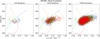 |
Figure 1 MCMC evolution plot showing three different states of the algorithm’s evolution for the slow ensemble. The starting points (shown as dots) of the four chains are drawn from a density that is over-dispersed with respect to the target density, and progressively they all end up sampling the same area of the parameter space defined by γ and w. The first plot shows 100 iterations, the second shows 1000 and the third shows 10,000 iterations. |
Out of the 10,000 samples from the four chains, we discard the burn-in phase (the first 900 samples) and thin them out by keeping 1 value every 30 (based on the computed autocorrelation time). Hence, each subset, for both the fast and slow cases, consists of 1256 samples after burn-in and thinning. This procedure is applied to all four subsets. Figure 2 illustrates the histograms of the marginal distributions of γ (on the left) and w (on the right) obtained from the four subsets in the fast (top) and slow (bottom) cases. Additionally, we report the cumulative distribution functions (CDFs) of the subsets in the same order (Figure 3). The PSRF score (described in Sect. 2.3) measures the ratio of intra-chain variance to inter-chain variance, indicating the level of convergence. If PSRF is approximately one, it suggests that the chains are sampling the same area of parameter space.
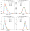 |
Figure 2 Probability distribution functions for solar wind speed w and drag parameter |

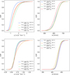 |
Figure 3 Cumulative distribution functions for solar wind speed w and drag parameter γ for fast (top) and slow (bottom) CMEs obtained leveraging four different folds of the dataset. The legend reports the mean value (avg), the standard deviation (std) and the PSRF score of the folds. |
The PSRF scores (reported in Figure 2) confirm the convergence of the chains in all cases. Additionally, the PDFs of the different subsets exhibit very similar mean values. We calculated the standard deviation of the average values of the PDFs, which is close to zero (reported in Figure 2). This indicates that the algorithm remains stable even with slight changes in the dataset. Based on these results, we can assert that the algorithm demonstrates robustness in terms of both convergence and stability. Thus, we can conclude that all the extracted samples belong to the same stationary posterior distribution, which is the desired posterior distribution that distinguishes the fast case from the slow case. Figure 4 shows the joint and marginal PDFs of γ and w.
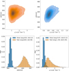 |
Figure 4 Posterior PDFs obtained from MCMC approach (upper left). Joint distribution of DBM parameters ( |


In the fast SW case, the posterior PDF of the solar wind speed (w) exhibits an average value of 600 km/s, while in the slow case, the average value of w is 430 km/s. In the fast SW case, the w values never fall below 500 km/s, while in the slow case, the highest value remains below 480 km/s. These results align with our assumed definition of CMEs propagating in slow and fast solar wind conditions. However, the marginal distributions of the drag parameter (γ) show noticeable differences. The drag parameter models the interaction between the CME and the solar wind. Figure 4 (lower left) illustrates that the algorithm tends to prefer larger values of γ in the fast SW ensemble case compared to the slow SW ensemble case. This observation is further supported by the slight correlation present in the posterior PDF of the slow data (Figure 4 (upper right)); as w increases, γ also increases. It is important to mention that the dispersion around the mean value in the two cases differs significantly. In the slow SW case, the values accepted by the MCMC algorithm tend to cluster more closely around the mean value, resulting in a smaller standard deviation. This difference can be attributed to the disparity in the ensemble sizes. Indeed, the slow SW case contains a larger number of elements than the fast SW case. The most stringent constraint placed on the ensemble approach is that a new sample (γ, w) is accepted if the proposed values allow solving the DBM equations for all CMEs in the ensemble. This condition makes the slow case more conservative, as the samples must fit a broader spectrum of events compared to the fast case. The resulting PDFs are then defined by the samples accepted under this assumption. Such samples, in principle, may not be the pair of values (γ, w) that best represent all the CMEs in the ensemble. To clarify this concept further, we provide additional details. In this framework, we assume that a probabilistic version of the DBM can model the dynamics of CMEs in interplanetary space. Thus, the evolution of each CME is described by the DBM equations, with the parameters (γ, w) represented as probability distributions rather than fixed values. The PDFs of the DBM parameters are, in principle, not identical for all CMEs, as the solar wind speed naturally varies because of the solar cycle, the solar rotation, as well as the different origin sources of the wind itself on the Sun. The assumption made in the ensemble approach leads to accepting DBM parameter samples that satisfy the model for all events, so the algorithm focuses on the areas of parameter space that best fit the ‘average’ behaviour of CMEs in the DBM framework. In the subsequent section, we will describe the results obtained using these PDFs for forecasting the transit time of CMEs.
4.1.1 Validation: transit time forecasting
One of the primary applications of P-DBM is to forecast the transit time and impact speed of CMEs with and their associated error. This can be achieved within a probabilistic framework by leveraging the estimated PDFs of the DBM parameters and, thus, generating an ensemble of value pairs ( ,
,  ). These values produce an ensemble of predictions for the transit time through the DBM. The average of the predictions and their standard deviation serve as transit time estimates and their associated error interval. In this work, we aim to test the forecasting capabilities of the PDFs extracted from the P-DBM framework. To ensure an unbiased evaluation, we employ a cross-validation technique. The dataset is divided into four training and test folds, where the training consists of randomly sampling 80% of the events from the dataset, and the remaining 20% of events serve as the test set. The training folds align with the four subsets described in the previous section. Hence, the PDFs are generated using the training set and the forecasting performances are evaluated on the test set. The four training subsets consist of 68 events for the slow case and 12 for the fast case, and four test subsets consist of 17 events in the slow case and 3 in the fast case. In total, we have 68 slow test events and 12 fast test events. This approach provides robustness to the performance evaluation of P-DBM and a relatively large test sample of CMEs to assess its performance. Using the P-DBM framework, we are able to generate a distribution of transit times as a result, rather than just isolated values. The average value within this distribution is treated as the estimated transit time (
 ) for the CMEs. In order for the model to be probabilistically reliable, we expect the true value of CME transit time (T) to fall within the confidence interval of 1σ in approximately 68% of the cases. Transit time forecasting results are summarised in Figure 5. The results show that the DBM manages to achieve prediction performances in line with the literature. The average Mean Absolute Errors (MAEs) of the predictions across the folds are approximately 10 h (slow case) and 7 h (fast case), with standard deviations of 3.4 h and 0.8 h, respectively (Figure 5 (left)). Additionally, the transit time forecast residuals (Figure 5 (left)) indicate a negligible bias in the fast case (−0.9 h) and a slight underestimation trend in the slow case (−4.55 h) in terms of mean error (ME). From a probabilistic perspective, the performance of the resulting P-DBM is relatively low. The true values of the transit time fall within the 1σ confidence intervals less than 68% of the cases for the slow and fast cases (Figure 5 (left)) We believe that the lack of consistency in the resulting confidence intervals is due to the structure of the inference method, which imposes strict constraints on the values of the DBM parameters, as mentioned at the end of Section 4.1. This leads to narrow posterior PDFs and the acceptance of samples carrying high errors in the likelihood. In the next section, we will explore the description of the individual approach.
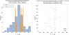 |
Figure 5 The transit time forecasting results with P-DBM obtained via the ensemble approach (left). Histogram of the residuals |


4.2 Individual approach
The ensemble approach yields PDFs of DBM parameters for a specific group of CMEs. With the individual approach we aim to further investigate the potential of the MCMC algorithm to obtain a specific P-DBM description for each CME event in the dataset. The structure of the algorithm is similar to that of the ensemble approach, but there are several distinctions, which are listed below. First, the input data for the algorithm pertains to individual CMEs, aiming to generate an output specific to each individual CME in the dataset. In this case, the output consists of PDFs of the DBM parameters for each CME event in the dataset. The limitations that required the samples to fit all CMEs of a specific ensemble are removed. We introduce a new free parameter for the MCMC algorithm, namely the initial velocity v0 of the CMEs. The reason is that the errors associated with the initial velocity in the dataset are very heterogeneous (some very large and some very small); this significantly penalises convergence. To prevent the algorithm from having too many degrees of freedom, we set the heliospheric distance to be 1 AU. Achieving convergence in the individual approach is more challenging compared to the ensemble case. In principle, the dynamics of each CME event are described by different parameters in the context of the DBM. Ideally, the data should drive the algorithm’s decisions by producing PDFs tailored to individual events. Therefore, in this case, we opt for weakly informative prior PDFs. For instance, we use a broad Gaussian distribution for the solar wind speed w with a mean of 400 km/s and a standard deviation of 200 km/s. The prior for v0 is a Gaussian distribution centred around the values stored in the dataset with a standard deviation of 200 km/s. For the drag parameter γ, we choose a log-normal PDF. These priors guide the algorithm to prefer sampling in parameter space regions close to the most probable parameter values. The convergence study remains unchanged: we run four chains with different initialization values for each CME and record the PSRF score values. At the end of the process, we discard the burn-in phase and thin the chains. This approach allows for the investigation of CMEs individually, meaning that the algorithm produces PDFs for the DBM parameters for each event in the dataset. For each event, we save statistical indicators describing these PDFs, such as the mean and standard deviation of the extracted samples, the convergence of the chains, and the acceptance rate of the algorithm. Since the algorithm is applied individually in this case, there is no a-priori distinction between CMEs belonging to the slow or fast ensemble. We define the PDFs of the slow ensemble and the fast ensemble by concatenating the samples of the CMEs labelled slow and fast, respectively, by Mugatwala et al. (2023). In essence, we construct an ensemble PDF (whether slow or fast) by aggregating all the individual PDFs (more specifically, all the samples defining such PDFs) of the CMEs belonging to the ensemble.
Figure 6 shows histograms of the marginal fast and slow PDFs of the DBM parameters obtained using the individual approach. The distribution of fast values for w appears noisier compared to the slow case due to the smaller number and potential heterogeneity of events in the fast ensemble. The results align with those obtained using the ensemble approach, but the marginal distributions are broader. The mean w values are 415 km/s and 514 km/s for the slow and fast cases, respectively. The average values for γ are  and
and  . This demonstrates that even with the individual approach, the algorithm tends to prefer values of solar wind speed
  for the slow case and
  for the fast case. Additionally, for γ, the fast case tends to assume higher values compared to the slow case, resulting in a distribution with a longer tail.
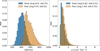 |
Figure 6 Histograms of marginal DBM parameter PDFs for the slow (blue) and fast ensemble (orange); obtained via individual approach. |
It is essential to highlight that the algorithm does not achieve convergence for all CME events. Some events exhibit non-robust convergence based on the PSRF score and acceptance rate data. Examining the most robust events identified by the algorithm is intriguing. We choose events with a PSRF score <1.05 for all free parameters and an acceptance rate greater than 5%. Out of the 213 CMEs in the dataset, 117 demonstrate good convergence according to the adopted convergence criteria. Among the 102 events categorized as “Nice Fits” by Mugatwala et al. (2023), 64 are determined to exhibit good convergence. There is an additional noteworthy observation. Inconsistencies are found when comparing the average values of the PDFs obtained through MCMC with the fast and slow labels used by Mugatwala et al. (2023).
Figure 7 illustrates that some events labelled as slow exhibit MCMC PDFs with mean values exceeding 500 km/s. Furthermore, most events with high solar wind speeds are recorded during the ascending or descending phase of the solar cycle. Consequently, a new labelling scheme for CMEs based on the average values of PDFs obtained via MCMC is adopted. Out of the 117 well-converged CMEs, 90 CMEs exhibit an average solar wind speed w < 500 km/s, and they are labelled as MCMC Slow, while 27 CMEs display an average solar wind speed w > 500 km/s and are labelled as MCMC fast.
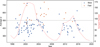 |
Figure 7 Scatter plot depicting the average solar wind speed ( |

Figure 8 displays the PDFs of the new ensembles alongside the previous ones (from Mugatwala et al. (2023) labels, in grey). The PDFs remain similar to the previous ones, ranging approximately the same interval of values. The distribution of w for the new slow ensemble shifts towards lower values, with an average of 400 km/s. In contrast, the new fast ensemble collects higher w samples, with an average of 580 km/s. A shift is also observed in the distributions of the drag parameter γ. The mean values of both MCMC and Mugatwala et al. (2023) ensembles are higher than before, and the gap between the two widens. Particularly, the tail of the distribution for the new fast ensemble is thicker and longer. The fast distribution remains noisy even with a larger sample of events, particularly for w. Finally, the individual approach PDFs are employed to test the forecasting capability of CME arrival time.
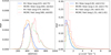 |
Figure 8 Histograms depicting the PDFs of marginal DBM parameters for the MCMC slow ensemble (MCMC slow), and the MCMC fast ensemble (MCMC fast) obtained via the individual approach. We also report Mugatwala et al. (2023) ensembles PDFs (M-I slow and fast) for comparison. |
4.2.1 Validation: transit time forecasting
In this section, we present the results of transit time forecasting of CMEs using the Individual approach with P-DBM. The individual approach allows us to obtain specific PDFs for each CME event in the dataset, which can then be used to define PDFs representing ensembles of CMEs with common characteristics. We defined two versions of the PDFs for the slow and fast ensembles. In the first version, the PDFs are constructed using the labels from Mugatwala et al. (2023) as in the ensemble approach, resulting in 87 slow events and 15 fast events. In the second version, we expanded the dataset by including all CMEs that showed good convergence criteria, resulting in 90 slow events and 27 fast events. To evaluate the forecasting performance, we used a 4-fold cross-validation method, similar to the ensemble approach. The dataset was divided into four sub-ensembles: three for training and validation to define the PDFs and one as a test set for evaluation. For the first version, each training set consisted of 68 slow events and 12 fast events, while each test set consisted of 17 slow events and 3 fast events. For the second version, the training sets consisted of 72 slow events and 22 fast events, while the test sets consisted of 18 slow events and 5 fast events. The forecasting results are summarised in Figure 9 for both versions.
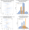 |
Figure 9 The transit time forecasting results with P-DBM obtained via individual approach (right). Scatter-plot of the residuals |


The graphs in the figure show the forecasting results obtained using the individual approach with P-DBM. The upper graphs represent the ensembles defined by Mugatwala et al. (2023) labelling, while the lower graphs represent the ensembles obtained by relabeling via MCMC. Overall, the forecasting performance of the individual approach is consistent with that of the ensemble approach. The MAE values are comparable, indicating similar levels of accuracy. In the first version of the PDFs, the slow ensemble shows slightly lower average error, while this is higher for the fast ensemble. Although the model exhibits reliability from a probabilistic perspective, the extensive error bars associated with the transit time estimates can be attributed to the broadness of the PDFs. Similar to the ensemble approach, the model tends to underestimate the transit time. However, the results for the MCMC ensemble PDFs are less promising. The MAE values are higher, indicating larger errors; in particular, the overcast for fast CMEs is much more evident. This discrepancy is further evident in the probabilistic performance, as the 1σ confidence intervals are not respected. Conversely, the forecasting performance for the slow ensemble remains satisfactory, considering the larger size of the test set.
5 Discussion and conclusions
In this section, we present a discussion of the results obtained from both the ensemble approach and the individual approach in producing PDFs for DBM parameters and forecasting the transit time of CMEs using the P-DBM framework. To evaluate the performance of transit time forecasting, we used a cross-validation technique. The P-DBM framework leveraged the PDFs of the DBM parameters to generate ensemble predictions for transit time. In the ensemble approach, we employed an MCMC algorithm to estimate the posterior distributions of the DBM parameters for an ensemble of CMEs. The algorithm was designed to only accept candidate parameter sets that satisfied the DBM equations for all CMEs within the group. This approach allowed us to obtain a distribution of parameters that represents the collective behaviour of the CMEs with common features. We examined the posterior distributions of the drag parameter (γ) and the solar wind speed (w) for two categories of CMEs: either interacting with slow (slow ensemble) or fast (fast ensemble) solar wind. The resulting PDFs provided an average representation of the behaviour of CMEs propagating in different heliospheric conditions. These PDFs yielded transit time predictions that showed relatively good performance in terms of Mean Absolute Error (MAE), considering the size of the test set and the simplicity of the model. However, the model proved to be probabilistically unreliable. In contrast, the individual approach aimed to obtain specific PDFs for each CME event in the dataset. We introduced the initial velocity v0 as a free parameter and employed weakly informative prior distributions for the DBM parameters. The algorithm was applied individually to each event, and the resulting PDFs were used to define PDFs for the slow and fast ensembles of CMEs. The evaluation of the forecasting results demonstrated similar performance between the ensemble approach and the individual approach, with comparable MAEs. Considering the advantages and disadvantages of each approach, the individual approach exhibited greater probabilistic robustness, providing a more reliable representation of the uncertainty associated with the transit time estimates. However, the error bars associated with the transit time estimates obtained through the individual approach were relatively large, indicating significant uncertainty in the predictions. In Table 1, we collect the primary descriptors of the PDFs obtained in this work. Additionally, we compare them with the results obtained in previous works. Overall, the PDFs obtained in this study align with the findings of previous research. CMEs propagating in slow solar wind conditions exhibit PDFs centered around low values of w (w < 500 km/s). Conversely, CMEs propagating in fast solar wind are characterized by PDFs centred at higher greater of w (w > 500 km/s). This observation holds true for the earlier studies as well (e.g. in Napoletano et al., 2018; Mugatwala et al., 2023), with the sole exception being the fast case in N2, where the average value for the PDF of w is found to be 490 km/s. Regarding the γ parameter, the discussion becomes more intricate. A notable distinction is observed in the γ PDFs when employing the ensemble approach versus the individual approach. Within the group approach, the algorithm appears to indicate a trend of higher γ values being associated with higher values of w. This is evident as the γ mean value of the fast case is notably greater than that of the slow case. Moreover, the joint distribution of the slow case (Fig. 4 top-right) also reveals a slight positive correlation between w and γ. Conversely, when considering the individual approach, this outcome is less evident. The disparity between the PDFs of γ in the fast and slow cases is not pronounced enough to strongly imply a distinct characterization in terms of the drag parameter. It is crucial to highlight that the sample of labelled CMEs as traveling in fast solar wind is exceedingly limited. This limitation poses a challenge when attempting to draw robust conclusions regarding the ensemble of fast cases. The positive correlation observed in the group approach may potentially arise as a mathematical compensation effect, driven by the stringent constraints inherent to that approach. Furthermore, Table 2 displays the results for CME transit time forecasting as presented in this research, along with the corresponding findings from other works utilizing the DBM framework, namely, the P-DBM and the drag-based ensemble model (DBEM). We also present results achieved by utilizing machine learning models, in order to provide a broader range of comparisons. Generally, comparing results across various studies is challenging. This difficulty primarily arises from the fact that different criteria are typically employed to create datasets for building or training models and subsequently assessing their performance. This issue is particularly pronounced in data-driven methods, as the input space defines the phenomenon one aims to represent. Additionally, the size of the sample has an impact on the evaluation metrics. To provide a comprehensive perspective on the results across different studies, additional information on the models employed, the validation technique, and the size of the test set are also included. It is worth noting the intriguing fact that the outcomes obtained for both the ensemble approach and the individual approach (specifically, M-I slow and fast) stem from the same training/test sets and employ the same evaluation methodology, rendering them readily comparable.
This table presents the moments of the distributions obtained in the current study for the DBM parameters w and γ, along with a comparative analysis against findings from prior research. The reported values comprise the mean and standard deviation of the distributions.
The table compiles the Mean Absolute Error (MAE) results achieved in this study for transit time forecasting and compares them with those obtained in earlier works that employed the DBM framework.
It is important to acknowledge that data-driven techniques heavily rely on the quality of the available data. Unfortunately, the data we have for modelling CMEs are affected by recurring errors, e.g. due to the approximation or the erroneous CME/ICME association. More importantly, the number of CME events employed here is limited, highly influencing the results. These limitations became evident when comparing the results between the slow SW and fast SW cases. The algorithm struggled to provide a comprehensive description of the fast SW ensemble due to the smaller number of available CME events compared to the slow case. Furthermore, this work was based on the assumption that there are only two types of CMEs, which is a strong approximation. The ensemble approach imposed restrictive conditions for accepting samples, ensuring they solve the DBM equations for all CMEs. However, it is likely that the DBM is not optimal to precisely describe all CME events in the dataset. On the other hand, the individual approach, which utilized PDFs obtained for each CME event, allowed more flexibility but carried the risk of losing the collective characteristics in favour of CME-specific ones. Moving forward, these findings suggest the potential for testing the algorithm on various ensembles of CMEs, corresponding to different phases of the solar cycle. Additionally, our analysis indicates a tendency for the algorithm to associate higher values with the solar wind speed in the ascending and descending phases of the solar cycle, as observed in Figure 7. Finally, we employed an MCMC algorithm based on the popular Metropolis-Hastings method. Exploring more sophisticated MCMC techniques (e.g. Goodman & Weare, 2010) could enhance sampling efficiency and acceptance rates, leading to more appropriate PDFs.
In conclusion, the DBM provides a valuable and efficient tool for CME forecasting. Enhancing the characterization of this model is essential for advancing CME forecasting efforts. Bayesian methods, particularly the MCMC algorithm, show promise in the probabilistic characterization of the DBM. Further exploration of these Bayesian approaches is warranted to improve our understanding and utilization of the DBM for CME forecasting.
Acknowledgments
This research work has been a part of the Space Weather Awareness Training NETwork (SWATNet) project. SWATNet has received funding from the European Union’s Horizon 2020 research and innovation programme under the Marie Sklodowska-Curie Grant Agreement No. 955620. This research has been also carried out in the framework of the CAESAR project, supported by the Italian Space Agency and the National Institute of Astrophysics through the ASI–INAF n.2020-35-HH.0 agreement for the development of the ASPIS prototype of the scientific data centre for Space Weather. This research has received financial support from the European Union’s Horizon 2020 research and innovation program under grant agreement No. 824135 (SOLARNET). E.C. was partially supported by NASA grants 80NSSC20K1580 “Ensemble Learning for Accurate and Reliable Uncertainty Quantification” and 80NSSC20K1275 “Global Evolution and Local Dynamics of the Kinetic Solar Wind”. R.E. is grateful to STFC (UK, grant No. ST/M000826/1), NKFIH OTKA (Hungary, grant No. K142987) and the ISSI-Beijing programme “Step forward in solar flare and Coronal Mass Ejection (CME) forecasting” for the support received. D.D.M. is grateful to the Italian Space Weather Community (SWICo). R.F. acknowledges support from the project “EVENTFUL” (ANR-20-CE30-0011), funded by the French “Agence Nationale de la Recherche” – ANR through the program AAPG-2020. The editor thanks two anonymous reviewers for their assistance in evaluating this paper.
The catalogue can be found at https://cdaw.gsfc.nasa.gov/CME_list/.
References
- Brooks S 1998. Markov chain Monte Carlo method and its application. J R Stat Soc Series D (the Statistician) 47(1), 69–100. https://doi.org/10.1111/1467-9884.00117. [Google Scholar]
- Brooks SP, Gelman A. 1998. General methods for monitoring convergence of iterative simulations. J Comput Graph Stat 7(4), 434–455. https://doi.org/10.1080/10618600.1998.10474787. [Google Scholar]
- Brooks S, Gelman A, Jones G, Meng X-L. 2011. Handbook of Markov Chain Monte Carlo, CRC Press. [CrossRef] [Google Scholar]
- Čalogović J, Dumbović M, Sudar D, Vršnak B, Martinić K, Temmer M, Veronig AM. 2021. Probabilistic drag-based ensemblemodel (DBEM) evaluation for heliospheric propagation of CMEs. Sol Phys 296(7), 114. https://doi.org/10.1007/s11207-021-01859-5. [CrossRef] [Google Scholar]
- Camporeale E. 2019. The challenge of machine learning in space weather: nowcasting and forecasting. Space Weather 17(8), 1166–1207. https://doi.org/10.1029/2018SW002061. [CrossRef] [Google Scholar]
- Cargill PJ. 2004. On the aerodynamic drag force acting on interplanetary coronal mass ejections. Sol Phys 221(1), 135–149. https://doi.org/10.1023/B:SOLA.0000033366.10725.a2. [CrossRef] [Google Scholar]
- Del Moro D, Napoletano G, Forte R, Giovannelli L, Pietropaolo E, Berrilli F. 2019. Forecasting the 2018 February 12th CME propagation with the P-DBM model: a fast warning procedure. Ann Geophys 62(4), GM456–GM456. https://doi.org/10.4401/ag-7750. [Google Scholar]
- Dumbović M, Čalogović J, Vršnak B, Temmer M, Mays ML, Veronig A, Piantschitsch I. 2018. The drag-based ensemble model (DBEM) for coronal mass ejection propagation. Astrophys J 854(2), 180. https://doi.org/10.3847/1538-4357/aaaa66. [CrossRef] [Google Scholar]
- Gelman A, Rubin DB. 1992. Inference from iterative simulation using multiple sequences. Stat Sci 7(4), 457–472. https://doi.org/10.1214/ss/1177011136. [Google Scholar]
- Goodman J, Weare J. 2010. Ensemble samplers with affine invariance. Commun Appl Math Comput Sci 5(1), 65–80. https://doi.org/10.2140/camcos.2010.5.65. [CrossRef] [Google Scholar]
- Gopalswamy N, Lara A, Lepping R, Kaiser M, Berdichevsky D, Cyr OSt . 2000. Interplanetary acceleration of coronal mass ejections. Geophys Res Lett 27(2), 145–148. https://doi.org/10.1029/1999GL003639. [CrossRef] [Google Scholar]
- Gopalswamy N, Mäkelä P, Xie H, Akiyama S, Yashiro S. 2009. CME interactions with coronal holes and their interplanetary consequences. J Geophys Res Space Phys 114(A3). https://doi.org/10.1029/2008JA013686. [Google Scholar]
- Hastings WK. 1970. Monte Carlo sampling methods using Markov chains and their applications. Biometrika 57(1), 97–109. https://doi.org/10.1093/biomet/57.1.97. [NASA ADS] [CrossRef] [Google Scholar]
- Huang X, Wang H, Xu L, Liu J, Li R, Dai X. 2018. Deep learning based solar flare forecasting model. I. Results for line-of-sight magnetograms. Astrophys J 856(1), 7. https://doi.org/10.3847/1538-4357/aaae00. [CrossRef] [Google Scholar]
- Jones GL, Qin Q. 2022. Markov chain Monte Carlo in practice. Annu Rev Stat Appl 9(1), 557–578. https://doi.org/10.1146/annurev-statistics-040220-090158. [CrossRef] [Google Scholar]
- Korsós MB, Erdélyi R, Liu J, Morgan H. 2021. Testing and validating two morphological flare predictors by logistic regression machine learning. Front Astron Space Sci 7, 113. https://doi.org/10.3389/fspas.2020.571186. [Google Scholar]
- Liu J, Ye Y, Shen C, Wang Y, Erdélyi R. 2018. A new tool for CME arrival time prediction using machine learning algorithms: CAT-PUMA. Astrophys J 855(2), 109. https://doi.org/10.3847/1538-4357/aaae69. [Google Scholar]
- Metropolis N, Rosenbluth AW, Rosenbluth MN, Teller AH, Teller E. 1953. Equation of state calculations by fast computing machines. J Chem Phys 21(6), 1087–1092. https://doi.org/10.1063/1.1699114. [CrossRef] [Google Scholar]
- Mugatwala R, Chierichini S, Francisco G, Napoletano G, Foldes R, Giovannelli L, Gasperis GD, Camporeale E, Erdélyi R, Moro DD. 2023. A catalogue of observed geo-effective CME/ICME characteristics. https://doi.org/10.48550/arXiv.2311.13429. [Google Scholar]
- Napoletano G, Forte R, Del Moro D, Pietropaolo E, Giovannelli L, Berrilli F. 2018. A probabilistic approach to the drag-based model. J Space Weather Space Clim 8, A11. https://doi.org/10.1051/swsc/2018003. [CrossRef] [EDP Sciences] [Google Scholar]
- Napoletano G, Foldes R, Camporeale E, de Gasperis G, Giovannelli L, Paouris E, Pietropaolo E, Teunissen J, Tiwari AK, Del Moro D. 2022. Parameter distributions for the drag-based modeling of CME propagation. Space Weather 20(9), e2021SW002925. https://doi.org/10.1029/2021SW002925. [CrossRef] [Google Scholar]
- Odstrcil D. 2003. Modeling 3-D solar wind structure. Adv Space Res 32(4), 497–506. https://doi.org/10.1016/S0273-1177(03)00332-6. [CrossRef] [Google Scholar]
- Owens M, Cargill P. 2004. Predictions of the arrival time of coronal mass ejections at 1 AU: an analysis of the causes of errors. Ann Geophys 22(2), 661–671. https://doi.org/10.5194/angeo-22-661-2004. [CrossRef] [Google Scholar]
- Paouris E, Čalogovic′ J, Dumbovic′ M, Mays ML, Vourlidas A, Papaioannou A, Anastasiadis A, Balasis G. 2021. Propagating conditions and the time of ICME arrival: a comparison of the effective acceleration model with ENLIL and DBEM models. Sol Phys 296(1), 12. https://doi.org/10.1007/s11207-020-01747-4. [CrossRef] [Google Scholar]
- Piersanti M, De Michelis P, Del Moro D, Tozzi R, Pezzopane M, et al. 2020. From the Sun to Earth: effects of the 25 August 2018 geomagnetic storm. Ann Geophys 38(3), 703–724. https://doi.org/10.5194/angeo-38-703-2020. [CrossRef] [Google Scholar]
- Pomoell J, Poedts S. 2018. EUHFORIA: European heliospheric forecasting information asset. J Space Weather Space Clim 8, A35. https://doi.org/10.1051/swsc/2018020. [Google Scholar]
- Pulkkinen T. 2007. Space weather: terrestrial perspective. Living Rev Sol Phys 4(1), 1–60. https://doi.org/10.12942/lrsp-2007-1. [CrossRef] [Google Scholar]
- Richardson IG, Cane HV. 2010. Near-Earth interplanetary coronal mass ejections during solar cycle 23 (1996–2009): catalog and summary of properties. Sol Phys 264(1), 189–237. https://doi.org/10.1007/s11207-010-9568-6. [CrossRef] [Google Scholar]
- Rollett T, Möstl C, Isavnin A, Davies JA, Kubicka M, Amerstorfer UV, Harrison RA. 2016. ElEvoHI: a novel CME prediction tool for heliospheric imaging combining an elliptical front with drag based model fitting. Astrophys J 824(2), 131. https://doi.org/10.3847/0004-637X/824/2/131. [CrossRef] [Google Scholar]
- Schwenn R. 2006. Space weather: the solar perspective. Living Rev Sol Phys 3(1), 1–72. https://doi.org/10.12942/lrsp-2006-2. [CrossRef] [Google Scholar]
- Shi T, Wang Y, Wan L, Cheng X, Ding M, Zhang J. 2015. Predicting the arrival time of coronal mass ejections with the graduated cylindrical shell and drag force model. Astrophys J 806(2), 271. https://doi.org/10.1088/0004-637X/806/2/271. [CrossRef] [Google Scholar]
- Temmer M. 2021. Space weather: the solar perspective. Living Rev Sol Phys 18(1), 4. https://doi.org/10.1007/s41116-021-00030-3. [CrossRef] [Google Scholar]
- Vourlidas A, Patsourakos S, Savani N. 2019. Predicting the geoeffective properties of coronal mass ejections: current status, open issues and path forward. Philos Trans R Soc A 377(2148), 20180096. https://doi.org/10.1098/rsta.2018.0096. [CrossRef] [Google Scholar]
- Vršnak B, Žic T, Vrbanec D, Temmer M, Rollett T, et al. 2013. Propagation of interplanetary coronalmass ejections: the drag-based model. Sol Phys 285(1–2), 295–315. https://doi.org/10.1007/s11207-012-0035-4. [CrossRef] [Google Scholar]
- Wang Y, Liu J, Jiang Y, Erdélyi R. 2019. CME arrival time prediction using convolutional neural network. Astrophys J 881(1), 15. https://doi.org/10.3847/1538-4357/ab2b3e. [CrossRef] [Google Scholar]
- Yashiro S, Gopalswamy N, Michalek G, OCSt Cyr, Plunkett SP, Rich NB, Howard RA. 2004. A catalog of white light coronal mass ejections observed by the SOHO spacecraft J Geophys Res Space Phys 109(A7). https://doi.org/10.1029/2003JA010282. [CrossRef] [Google Scholar]
Cite this article as: Chierichini S, Francisco G, Mugatwala R, Foldes R, Camporeale E, et al. 2024. A Bayesian approach to the drag-based modelling of ICMEs. J. Space Weather Space Clim. 14, 1. https://doi.org/10.1051/swsc/2023032.
All Tables
This table presents the moments of the distributions obtained in the current study for the DBM parameters w and γ, along with a comparative analysis against findings from prior research. The reported values comprise the mean and standard deviation of the distributions.
The table compiles the Mean Absolute Error (MAE) results achieved in this study for transit time forecasting and compares them with those obtained in earlier works that employed the DBM framework.
All Figures
|
Figure 1 MCMC evolution plot showing three different states of the algorithm’s evolution for the slow ensemble. The starting points (shown as dots) of the four chains are drawn from a density that is over-dispersed with respect to the target density, and progressively they all end up sampling the same area of the parameter space defined by γ and w. The first plot shows 100 iterations, the second shows 1000 and the third shows 10,000 iterations. |
| In the text | |
|
Figure 2 Probability distribution functions for solar wind speed w and drag parameter |
| In the text | |
|
Figure 3 Cumulative distribution functions for solar wind speed w and drag parameter γ for fast (top) and slow (bottom) CMEs obtained leveraging four different folds of the dataset. The legend reports the mean value (avg), the standard deviation (std) and the PSRF score of the folds. |
| In the text | |
|
Figure 4 Posterior PDFs obtained from MCMC approach (upper left). Joint distribution of DBM parameters ( |
| In the text | |
|
Figure 5 The transit time forecasting results with P-DBM obtained via the ensemble approach (left). Histogram of the residuals |
| In the text | |
|
Figure 6 Histograms of marginal DBM parameter PDFs for the slow (blue) and fast ensemble (orange); obtained via individual approach. |
| In the text | |
|
Figure 7 Scatter plot depicting the average solar wind speed ( |
| In the text | |
|
Figure 8 Histograms depicting the PDFs of marginal DBM parameters for the MCMC slow ensemble (MCMC slow), and the MCMC fast ensemble (MCMC fast) obtained via the individual approach. We also report Mugatwala et al. (2023) ensembles PDFs (M-I slow and fast) for comparison. |
| In the text | |
|
Figure 9 The transit time forecasting results with P-DBM obtained via individual approach (right). Scatter-plot of the residuals |
| In the text | |
Current usage metrics show cumulative count of Article Views (full-text article views including HTML views, PDF and ePub downloads, according to the available data) and Abstracts Views on Vision4Press platform.
Data correspond to usage on the plateform after 2015. The current usage metrics is available 48-96 hours after online publication and is updated daily on week days.
Initial download of the metrics may take a while.