| Issue |
J. Space Weather Space Clim.
Volume 15, 2025
Topical Issue - Swarm 10-Year Anniversary
|
|
|---|---|---|
| Article Number | 26 | |
| Number of page(s) | 11 | |
| DOI | https://doi.org/10.1051/swsc/2025022 | |
| Published online | 30 June 2025 | |
Technical Article
A climatological model of the equatorial electrojet based on Swarm satellite magnetic intensity observations
1
Division of Geomagnetism and Geospace, DTU Space, Technical University of Denmark, Centrifugevej 356, DK-2800 Kongens Lyngby, Denmark
2
Cooperative Institute for Research in Environmental Sciences, University of Colorado Boulder, 216 UCB, Boulder, CO, USA
3
ESA–ESRIN, via Galileo Galilei 2, I-00044 Frascati, Italy
* Corresponding author: This email address is being protected from spambots. You need JavaScript enabled to view it.
Received:
20
November
2024
Accepted:
11
May
2025
Abstract
The Equatorial Electrojet (EEJ) is a spatially localized electric current in the ionospheric dynamo region, flowing along the magnetic dip equator at an altitude of about 110 km, mainly on the dayside. Previous empirical models of the EEJ were based on magnetic intensity observations from the Ørsted, CHAMP, and SAC-C satellites. However, with the launch of the Swarm satellite trio in November 2013, a considerable amount of new data is available. We use latitudinal profiles of EEJ sheet current densities based on magnetic intensity measurements of the Swarm A and B satellites to construct a climatological model of the EEJ. This model describes sheet current density variations with local time, longitude, season, lunar phase, and the F10.7 solar flux. We validate our model with independent EEJ current density estimates from the Swarm C and CSES satellites.
Key words: Geomagnetism / Equatorial electrojet / Swarm satellites / Inverse problems
Now at University of Oslo, Norway
© N. Olsen et al., Published by EDP Sciences 2025
 This is an Open Access article distributed under the terms of the Creative Commons Attribution License (https://creativecommons.org/licenses/by/4.0), which permits unrestricted use, distribution, and reproduction in any medium, provided the original work is properly cited.
1 Background
Atmospheric winds and tidal oscillations in the ionospheric dynamo region (100–150 km altitude) cause an electrical current system that is referred to as the Sq current system (e.g. Chapman & Bartels, 1940; Matsushita, 1967; Yamazaki & Maute, 2016). It is responsible for daily magnetic field variations that can be measured at the Earth’s surface and by low-Earth orbiting satellites. The Sq current system can be roughly described by two vortices, one centred on each dayside hemisphere at around ±35° magnetic latitude and local noon, which tangentially meet each other at the magnetic dip equator. Because of the specific configuration of the ambient magnetic field near the equator, the local eastward Sq currents are amplified, creating the “Equatorial Electrojet” (EEJ) (e.g. Matsushita, 1967; Onwumechili, 1967; Jadhav et al., 2002; Yamazaki & Maute, 2016; Thomas et al., 2017; Lühr et al., 2021). Figure 1 shows the median height-integrated magnetic eastward EEJ currents for bins in Quasi-Dipole (QD) latitude (Richmond, 1995) and Local Time T (LT), based on 11 years of magnetic field observations from the Swarm satellites (details are given below). One can immediately recognise the eastward flowing “main body” (red) of the EEJ currents around the dip equator (QD latitude of 0°). Besides this “main body”, the EEJ often shows reverse (westward) current sidebands at ±5° QD latitude peaking around local noon. These sidebands are assumed to be caused by gradients of eastward zonal wind velocities with altitude and the resulting vertical shear (Liu et al., 2019; Lühr et al., 2021; Sreelakshmi et al., 2024).
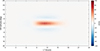 |
Figure 1 Median EEJ sheet current density as a function of Quasi-Dipole (QD) latitude and Local Time T based on 11 years of magnetic field observations from the Swarm A satellite. Eastward (i.e. positive) currents are indicated in red, and westward (i.e. negative) ones in blue. 10 A/km contour line interval. |
The strength of the EEJ can vary significantly over time and space. For example, while most often the EEJ at the dip equator flows in an eastward direction, in certain circumstances a westward so-called “counter equatorial electrojet” (CEJ) occurs (e.g. Vichare & Rajaram, 2011). Most commonly, CEJs appear during the morning hours (around 06 LT), when the nighttime westward electric field is still prevalent, but they can also develop in the afternoon.
The main external drivers of ionospheric current system variability are the Sun (e.g. variations in solar irradiation, solar activity, and geomagnetic disturbances) and variations in atmospheric processes (e.g. atmospheric tides and winds, Liu et al., 2019). The left part of Figure 2 shows the variation of the EEJ sheet current at the dip-equator as a function of Local Time T and geographic longitude ϕ, estimated from the same 11 years of Swarm satellite data. There is a clear longitudinal dependence of the EEJ, with four maxima and four minima, i.e. a longitudinal wavenumber of nϕ = 4.
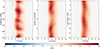 |
Figure 2 Left: Median EEJ sheet current density at the dip-equator as a function of Local Time T and longitude ϕ (left), season s (middle), and lunar phase ν, respectively. Same data as in Figure 1. |
The variation of the EEJ with season is illustrated in the middle panel of Figure 2. The EEJ has maxima around the equinoxes; however, in addition to this expected semi-annual variation, there is a secondary maximum during winter.
In addition to the solar forcing of the EEJ (which is mainly thermal) there is also a small lunar contribution to the EEJ, caused by gravitational forcing, which results in a thermospheric wind system that follows lunar Local Time Tl = T − ν, where lunar phase ν varies between 0 h and 24 h (ν = 0 h for New Moon and ν = 12 h for Full Moon). The right panel of Figure 2 reveals a lunar dependency with period 2ν, which is expected since the semi-diurnal M2 tidal mode is the largest lunar forcing term. Multiplication of semi-diurnal lunar thermospheric winds proportional to cos(2Tl) with ionospheric conductivity that is a function of solar Local Time T leads to Chapman’s phase law (e.g. Chapter 3.8.4 of Chapman & Bartels, 1940)
 (1)
(1)
where the quantity L can be e.g. magnetic field or sheet current density.
To understand the physics and structure of the EEJ, various empirical models of the EEJ have been derived using magnetic field observations from the ground and satellites (e.g. Jadhav et al., 2002; Doumouya et al., 2003; Alken & Maus, 2007). In 1999 and 2000, three satellites for geomagnetic surveying were launched: Ørsted, CHAMP, and SAC-C (e.g. Olsen et al., 2010). All three satellites carried a scalar absolute magnetometer and a vector magnetometer, providing highly accurate geomagnetic data for over a decade. SAC-C was slightly less successful, and no vector data were available due to missing attitude data. However, the data of all three satellites have been used extensively to investigate the EEJ and its variation with e.g. season and local time.
The hitherto most sophisticated model of the EEJ has been derived by Alken & Maus (2007) who constructed an empirical model based on CHAMP, Ørsted, and SAC-C satellite magnetic field observations, after removing model values of the core, lithospheric, and magnetospheric field from the data. The EEJ is modelled as a current sheet band at 108 km altitude, approximated by a set of line currents in the East-West direction. The model includes dependencies on longitude ϕ, Local Time T, season, and a linear dependence on solar activity. The authors use sine and cosine functions for describing variations in longitude and season. Dependence on Local Time is described by cubic B-spline functions with uniform knots. The original model (Alken & Maus, 2007) was later updated to include lunar variations as well (Alken, 2009). These models, termed respectively EEJM and EEJM-2, are available online1.
Since the release of the EEJM and EEJM-2 models, additional data have been collected by the Swarm and CSES satellite missions. In this paper, we use data from these two missions, along with records of auxiliary variables like geomagnetic and solar activity indices, to derive and validate a new climatological model of the EEJ.
2 Data
ESA’s Swarm satellite trio is dedicated to surveying the Earth’s magnetic field (Friis-Christensen et al., 2008; Olsen & Floberghagen, 2018). For this purpose, three identical satellites, respectively referred to as Alpha, Bravo, and Charlie (or A, B, and C), were put into near-polar low orbits on the 22nd of November 2013. Satellites Alpha and Charlie fly side-by-side (at a distance of about 50–150 km), thereby measuring the East-West gradient of the magnetic field. They orbit at slightly lower altitudes (initially at 462 km) than satellite Bravo (initially at 511 km). Each satellite carries a scalar magnetometer that provides highly accurate absolute measurements of the Earth’s magnetic field intensity, and a vector magnetometer co-mounted with a triple-head star imager to obtain attitude.
One of the Swarm Level-2 data products is the “Equatorial Electric Field” (EEF). This data product is derived from observations of the magnetic field intensity and includes latitudinal profiles of the height-integrated EEJ sheet current densities, the equatorial electric field strengths, and other related variables for each of the three Swarm satellites on an orbit-by-orbit basis. Details of the algorithm can be found in Alken et al. (2013, 2015). The currently operational Swarm EEF data product (EEFx_TMS_2F, where x=A, B, or C denotes the satellite) only includes dayside EEJ current density estimates. However, we applied a similar algorithm to magnetic measurements covering all local times and derived an extended dataset that includes both local day- and nighttime EEJ current density estimates for all three Swarm satellites for the period November 2013 to December 2024. These extended datasets have been used to derive the climatological model of the EEJ described in the present paper and allow us to determine a model of the EEJ covering all local times.
Eleven years’ worth of Swarm EEJ current density estimates, from the start of observations on the 25th of November 2013 until the 31st of December 2024, have been considered. The orbital period of Low-Earth-Orbiting (LEO) satellites is approximately 90 min, and thus approximately 32 equatorial crossing latitudinal profiles (16 when the satellite is northbound, and 16 when it is southbound) are available per day for each Swarm satellite. Each profile consists of 81 height-integrated magnetic eastward current values spanning the QD latitudes −20.0°, −19.5°, −19.0 °, …, −0.5°, 0.0°, +0.5°, …, +19.5°, +20.0°. In the following, we will concentrate on the EEJ at the dip-equator (QD latitude = 0°) but will extend to other latitudes in Section 6.
Data from the Swarm A and B satellites are used to derive the model. We validate our model with additional data that have not been used in constructing the model: in addition to data from Swarm C, we use current estimates derived by applying the EEF algorithm to magnetic intensity measurements taken by the Chinese Seismo-Electromagnetic Satellite (CSES-01) (Huang et al., 2018; Yang et al., 2021). This satellite was launched on the 2nd of February 2018 by the Chinese National Space Administration into a sun-synchronous orbit (02, resp. 14 LT) at an altitude of about 500 km. The satellite’s payload includes an absolute scalar magnetometer, the data of which, similarly to the Swarm satellite magnetic field observations, can be used to derive EEJ sheet current densities on an orbit-by-orbit basis. Because of the limited local time coverage (02/14 LT) this dataset is not suitable for deriving the full LT variation of the EEJ. However, CSES data are of particular interest for validating empirical models based on the Swarm data. In our study, we use CSES data between August 2018 and December 2024; however, there are gaps of several months duration for which no data are available.
Outliers have been removed from each of the four datasets used in our study (i.e. the extended Swarm A, B, and C datasets that cover all LT, and the CSES dataset for 02/14 LT) in the following way: let q1 and q99 be the 1st and 99th percentiles of each dataset, respectively. We removed data that were not in the range between q1 − 1.5Δq and q99 + 1.5Δq, with Δq = q99 − q1. The number of removed outliers approximately corresponds to what one would discard based on visual inspection. For the extended Swarm A and B datasets, 0.15% of the observations are removed, while the corresponding numbers for the CSES and Swarm C datasets are 0.35% and 0.10%, respectively.
3 Model parameterisation and model estimation
We assume that the EEJ sheet current density at a given QD latitude can be described by an expansion in periodic (sine and cosine) functions in Universal Time (UT) t (in radians, where t = 0 corresponds to 00:00 UT and t = 2π corresponds to 24:00 UT), geographic longitude ϕ (in radians), season s (in radians, counted from s = 0 on 20 March to s = 2π on 20 March of the following year), and lunar phase ν (in radians, where ν = 0 corresponds to New Moon and ν = π is Full Moon). The main component representing the daily temporal variation of the EEJ current density is a 24-hour periodic function of local time T = t + ϕ. This is because only one peak in the EEJ current density is observed per day around noon (cf. Fig. 1). However, since the EEJ peaks around local noon (T = 12 h) but almost vanishes during night between T = 18 h and T = 6 h, a proper description of the EEJ requires higher harmonics with periods that are integer fractions of the 24 h period. Following previous works for describing the LT-dependence of geomagnetic daily variations (e.g. Malin, 1973; Winch, 1981), we include nt = 4 daily harmonics (e.g. periods of 24 h, 12 h, 8 h, and 6 h).
To model the wavenumber-four longitudinal signature of the EEJ (cf. Fig. 2), we include longitudinal wavenumbers up to nϕ = 4. In addition, our model includes seasonal variations, including at least an annual periodic to capture summer/winter variations (Alken & Maus, 2007) and semi-annual periodic functions to model the expected peaks at the equinoxes (caused by maximum solar illumination near the equator). However, Figure 2 reveals shorter seasonal EEJ current density variations and thus our model includes seasonal variations of periods 12 months, 6 months, 4 months, and 3 months, i.e. up to ns = 4.
To account for the lunar tides, the corresponding periodic functions include a period of half a lunar phase ν, since the EEJ is strongest around New and Full Moon, resulting in a time dependence proportional to cos(−2ν). Note that the lunar phase variation “propagates” in the opposite direction of the daily solar variation (which is the reason for the negative sign of the time dependency in Eq. (1)). This is because the lunar tidal day (24.84 h) is longer than a solar tidal day (24 h).
Ignoring any variation with solar activity, the sheet current density J at a given QD latitude is modelled according to
![Mathematical equation: $$ J(t,\phi,s,\nu )=\sum_{p\stackrel{*}{=}0}^{{n}_t} \enspace \sum_{m\stackrel{*}{=}-{n}_{\phi }}^{{n}_{\phi }} \enspace \sum_{k\stackrel{*}{=}-{n}_s}^{{n}_s} \enspace \sum_{l\stackrel{*}{\in }{l}_{{sel}}} [{a}_{p,m,k,l}\enspace \mathrm{cos}\left({pt}+{m\phi }+{ks}+{l\nu }\right)\enspace +{b}_{p,m,k,l}\enspace \mathrm{sin}\left({pt}+{m\phi }+{ks}+{l\nu }\right)], $$](/articles/swsc/full_html/2025/01/swsc240083/swsc240083-eq2.gif) (2)
(2)
with lsel = [0, −2]. This periodic dependency in UT t, longitude ϕ, and season s is similar to that used in the Comprehensive Model (CM) series for describing ionospheric current systems (e.g. Sabaka et al., 2002). As already mentioned, the maximum order of the expansion in Universal Time t (nt = 4), in longitude ϕ (nϕ = 4), and in season s (ns = 4) have been selected after careful investigations of what is necessary to describe the observations (see also Fig. 2) and is further justified below. Counting the number of coefficients, one would naively expect (nt + 1) × (2nϕ + 1) × (2ns + 1) × 2 = 810 coefficients ap,m,k,l and a similar number for bp,m,k,l, resulting in 1620 coefficients in total. However, various combinations of p, m, k, and l are not allowed; for instance, b0,0,0,0 does not exist since the corresponding argument of the sine function is zero in that case. Invalid parameter combinations for both ap,m,k,l and bp,m,k,l occur if either (p = l = 0 and m < 0) or (p = l = m = 0 and k < 0). In combination with the exclusion of b0,0,0,0, this results in M = 1539 model parameters.
Collecting the N EEJ sheet current density data for a given QD latitude in the data vector d and the M model parameters in the model vector m, one can rewrite the problem as:
 (3)
(3)
where the design matrix G of dimension N × M is constructed following equation (2).
We solve for the model vector m using Iteratively Reweighted Least Squares (IRLS) with Huber weights with a tuning constant of 1.5 (cf. Huber, 1981):
 (4)
(4)
where the diagonal matrix W contains the Huber weights wi, i = 1, 2, … N. We thus minimize the weighted data misfit (see Eq. (7a)) where the data residual vector r = d − dmod with elements ri contains the differences between the actual observations d and the model predictions  .
.
The model parameterisation of equation (2), which we denote as Model 1, does not account for variations of the EEJ sheet current density with solar activity. We therefore consider a slightly more complex model, where the harmonic expansion of equation (2) is modulated with a linear function that depends on solar activity. Following Alken & Maus (2007) we use the solar flux proxy EUVAC (Extreme UltraViolet flux model for Aeronomic Calculations, Richards et al., 1994), defined as Fs = (F10.7 + F10.7A)/2, where F10.7 is the daily solar flux at 10.7 cm wavelength, and F10.7A is its 81-day running mean. Both F10.7 and Fs are given in “solar flux units” (s.f.u.). This leads to
![Mathematical equation: $$ \begin{array}{c}J(t,\phi,s,\nu,{F}_s)=(1+R\enspace {F}_s)\times \\ \sum_{p\stackrel{*}{=}0}^{{n}_t} \enspace \sum_{m\stackrel{*}{=}-{n}_{\phi }}^{{n}_{\phi }} \enspace \sum_{k\stackrel{*}{=}-{n}_s}^{{n}_s} \enspace \sum_{l\stackrel{*}{\in }{l}_{{sel}}} [{a}_{p,m,k,l}\enspace \mathrm{cos}\left({pt}+{m\phi }+{ks}+{l\nu }\right)\\ +{b}_{p,m,k,l}\enspace \mathrm{sin}\left({pt}+{m\phi }+{ks}+{l\nu }\right)].\end{array} $$](/articles/swsc/full_html/2025/01/swsc240083/swsc240083-eq6.gif) (5)
(5)
Co-estimation of the solar flux regression coefficient R, together with the expansion coefficients ap,m,k,l and bp,m,k,l, makes the problem weakly non-linear. It is solved iteratively (e.g. Chapter 9 of Aster et al., 2013) using starting values from the solution of the linear problem, equation (2), for ap,m,k,l and bp,m,k,l and R = 20 · 10−3 s.f.u. for the solar flux regression coefficient. The solution converged after 10 iterations. Note that all expansion coefficients are assumed to vary with the same regression coefficient R, which means that there is no change of “shape” of the current system but just a “scaling”. We denote this solution as Model 2, which consists of M = 1540 model parameters.
We finally estimate a third model for which each expansion coefficient ap,m,k,l and bp,m,k,l depends linearly on EUVAC:
![Mathematical equation: $$ \begin{array}{c}J(t,\phi,s,\nu,{F}_s)=\sum_{p\stackrel{*}{=}0}^{{n}_t} \enspace \sum_{m\stackrel{*}{=}-{n}_{\phi }}^{{n}_{\phi }} \enspace \sum_{k\stackrel{*}{=}-{n}_s}^{{n}_s} \enspace \sum_{l\stackrel{*}{\in }{l}_{{sel}}} \\ [\left({\bar{a}}_{p,m,k,l}+{\mathop{a}\limits^\tilde}_{p,m,k,l}\cdot {F}_s\right)\enspace \mathrm{cos}\left({pt}+{m\phi }+{ks}+{l\nu }\right)+\\ \left({\bar{b}}_{p,m,k,l}+{\mathop{b}\limits^\tilde}_{p,m,k,l}\cdot {F}_s\right)\enspace \mathrm{sin}\left({pt}+{m\phi }+{ks}+{l\nu }\right)].\end{array} $$](/articles/swsc/full_html/2025/01/swsc240083/swsc240083-eq7.gif) (6)
(6)
This doubles the number of model parameters and therefore the resulting Model 3 consists of M = 2 × 1539 = 3078 model parameters.
To assess the degree to which a model fits a given dataset, we use the root-mean-square error data misfit, rms, its weighted variant, wrms, and the Mean Absolute Deviation (MAD), defined as
 (7a)
(7a)
 (7b)
(7b)
 (8)
(8)
4 EEJ model sheet current density at the dip equator
Starting with the EEJ sheet current density at the dip-equator (0° QD latitude) we estimated the following three models: Model 1 follows the parameterisation of equation (2) (no dependency on solar activity, M = 1539 model parameters); Model 2 is based on equation (5) (linear scaling with EUVAC solar flux, M = 1540 model parameters), while Model 3 is based on equation (6) (each coefficient has separate linear dependence on EUVAC solar flux, M = 3078 model parameters). All three models are estimated from the combination of the extended Swarm A and B datasets.
For all three models, the condition number of the GTWG matrix in the final iteration is small (below 10), which indicates the stability of the solution for the chosen model parameterisation and no model regularisation was necessary.
Table 1 lists the obtained data misfit values. The IRLS estimation procedure minimises the “all day” weighted rms misfit wrms (bold number in the Table 1), but due to the different properties of the EEJ sheet current density during day and night, we also list data misfit statistics for daytime (06 – 18 LT) and nighttime (18 – 06 LT) conditions, respectively.
Unweighted root-mean-squared data misfit values (rms), Huber-weighted rms data misfit (wrms), and Mean Absolute Deviation (MAD), in A/km, for the three models of the EEJ sheet current density at the dip equator. Misfit values that are minimized by the inversion process are shown in bold.
Accounting for a common linear dependence on solar flux (Model 2) reduces the weighted rms misfit by about 5% compared to Model 1 (reduction from 15.64 A/km to 14.85 A/km), while only adding one single model parameter R. In comparison, allowing for each expansion coefficient ap,m,k,l and bp,m,k,l to vary with solar flux (and thus doubling the number of model parameters, Model 3) further reduces the weighted rms misfit by only 2% while doubling the number of model parameters. From this, we conclude that a linear scaling of the model current with solar flux, i.e. Model 2, is sufficient.
What is the impact of model parameterisation other than nt = ns = nϕ = 4, i.e. of changing the maximum order of the expansion of equation (5)? To investigate this, we derive three variants of Model 2, parametrised by (nt = 6, ns = nϕ = 4), (ns = 6, nt = nϕ = 4), and (nϕ = 6, nt = ns = 4), respectively. This change increases the number of model parameters by about 44% but results in almost no change in the rms data misfit: for the two models with either nt = 6 or ns = 6, the weighted data misfit decreases by about 0.1 A/km. For the third case, increasing nϕ from 4 to 6, the misfit decreased by 0.55 A/km (from wrms = 14.85 A/km to wrms = 14.30 A/km). However, this corresponds to a misfit reduction of only 4% despite increasing the number of model parameters by 44%. We, therefore, choose Model 2, with nt = ns = nϕ = 4, as our preferred solution and use this model parameterisation in the following.
The blue and red curves in Figure 3 represent the MAD as a function of Local Time between Model 2 and the data that have been used to derive that model (extended EEF data sets for Swarm A and B). The MAD statistics between the Swarm A data and the EEJM-2 model (Alken & Maus, 2007) derived from CHAMP satellite data, shown by the light blue curve, are slightly higher compared to those obtained with the model derived in this study.
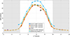 |
Figure 3 Mean Absolute Deviation (MAD) of observations minus model predictions at the dip equator as a function of Local Time for the various data sets. Grey areas represent nighttime hours. |
The maxima around local noon indicate the highest scatter (i.e. variations between observed and modelled values) during daytime when the EEJ sheet current densities are largest. Given a typical strength of the EEJ sheet currents of 100 A/km during noon (cf. Fig. 2), the MAD of 20–30 A/km indicates a large orbit-to-orbit variability, i.e. the EEJ sheet current density of a particular orbit can be rather different from that of the following orbit about 90 min later. This is confirmed by the relatively low correlation coefficient ρ ≈ 0.6 of the EEJ between two consecutive equatorial crossings, shown by the blue curve in the left part of Figure 4 for the extended Swarm A dataset. Interestingly, the correlation is slightly higher in the morning compared to the evening.
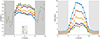 |
Figure 4 Left: Correlation between observed (extended Swarm A dataset) and modelled sheet current density at the dip equator as a function of Local Time, after averaging over K consecutive values. Right: Same, but for the MAD between observed and modelled values. Grey areas represent nighttime hours. |
To investigate this orbit-to-orbit variability further, we calculate misfit statistics and correlation coefficients after averaging observed (extended Swarm A dataset) and modelled EEJ current estimates over K consecutive orbits. Averaging over K = 7 values (which corresponds to averaging over 7 × 90 min = 10.5 h) reduces the MAD during noon by almost a factor of 2 (from 28 A/km to 15 A/km) and increases the correlation coefficient to ρ ≈ 0.7. Averaging over K = 30 consecutive orbits (corresponding to 2 days) lead to ρ = 0.9 and reduce the MAD to less than 10 A/km. From this, we conclude that our model can reproduce changes in the EEJ occurring on time scales longer than a few days – as expected for a good climatological model – but is not able to capture orbit-to-orbit variations.
Figure 5 shows the EEJ sheet current density at the dip-equator as a function of longitude ϕ and Local Time T, for different seasons, as given by Model 2. Several aspects are worthwhile to notice: a) the EEJ is strongest during equinoxes and weakest during solstices; b) the peak of the EEJ current occurs slightly before local noon; c) although there is a rather sharp onset of the EEJ between 07 and 08 LT for all longitudes, post-noon features of the EEJ differ with longitude. In the morning, westward currents (i.e. morning CEJs) seem to be present at almost all longitudes, with peaks around the longitudes where the eastward daytime EEJ is relatively weak. It has been suggested that the strong morning CEJs are due to the relatively high prevalence of meteor incidences in this period (Alken & Maus, 2007). Meteoric dust particles from meteor ablation trails create a negatively charged layer in the lower E-region. Thus, a downward electric field is established that supports a westward current. The occurrence of evening CEJs is less consistent with season and longitude.
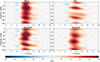 |
Figure 5 Model EEJ sheet current density at the dip-equator (QD latitude = 0°) as a function of longitude ϕ and Local Time T, for different seasons and a mean solar flux of |

5 Model validation
To validate our model, we calculate the misfit statistics between model predictions and observations that were not used in deriving the model. Figure 3 shows that the misfit of the Swarm C (orange curve) and CSES data sets (magenta dot) are comparable to those of the Swarm A and B data (red and blue) that have been used for estimating the model. We only show misfit values for 14 LT since the CSES satellite operates from a sun-synchronous orbit, and dayside EEJ profiles are only available for 14 LT. Surprisingly, the MAD misfit to CSES data, which have not been used in the model estimation, is lower than those for the Swarm A and B data from which the model was derived. This, however, is likely due to the subset of years for which CSES data are available; selecting Swarm B data (which flies at a similar altitude as CSES) for the same years, and Local Time window as CSES leads to a comparable low misfit (green dot).
The similarity of MAD misfit statistics for the different data sets – regardless of whether they have been used in model determination or not – gives us confidence in the validity of our model. Daytime MAD data misfit values of 25 A/km and higher indicate a relatively large scatter, given the typical noon sheet current densities of 50–100 A/km. However, it is important to remember that we derive a climatological model of the EEJ sheet current densities and that the uncertainty of predicted model values is much smaller than the obtained data misfit to single orbits.
To investigate this further, we derived two independent models using the same model parameterisation as Model 2, but estimated either only from the Swarm A data set (resulting in Model 2A) or only from the Swarm B data set (Model 2B). These two models are validated by comparing misfit statistics for the data sets used to estimate that model (e.g. Swarm A for Model 2A) and the corresponding independent data set (in that case, Swarm B data). The results, listed in Table 2, confirm that misfit statistics to independent data are very similar to those used for model estimation.
Unweighted root-mean-squared data misfit values (rms), Huber-weighted rms data misfit (wrms), and Mean Absolute Deviation (MAD), in A/km, for the Models 2A (derived entirely using data from Swarm Alpha) and 2B (using only Swarm Bravo data), respectively. The first column, entitled “Model 2A – A data”, lists statistics for the Swarm Alpha data (which were used in deriving this model), whereas the second column, “Model 2A – B data”, lists statistics for the independent Swarm Bravo data (not used in model construction). Similar for the third and fourth columns. Misfit values that are minimized by the inversion process are shown in bold.
The difference between the two models 2A and 2B is indicative of the uncertainty of the combined Model 2. Figure 6 presents this difference in sheet current density at the dip-equator for different seasons. Comparison with Figure 7 shows that the uncertainty of the model predictions (typical values are well below 10 A/km) is considerably smaller than the actual model predictions (of 100 A/km and more during noon). These results give us further confidence in the robustness of our climatological model of the EEJ sheet current densities.
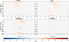 |
Figure 6 Similar to Figure 2 but for model uncertainty, determined as the difference between Model 2A and Model 2B. |
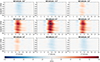 |
Figure 7 Model EEJ sheet current density as a function of longitude ϕ and Local Time T, for different QD latitudes. Calculated for March equinoxes, New Moon (lunar phase ν = 0), and a mean solar flux of |

 |
Figure 8 Observed and modelled sheet current density for the first half of 2018 (solar minimum, mean solar flux |


6 The EEJ model between ±20° QD latitude
Until now, we only looked at the EEJ at the dip-equator (0° QD latitude). We now apply the model parameterisation of equation (5) to all 81 EEJ sheet current estimates based on the combined extended Swarm A and B datasets, spanning QD latitudes between −20° and +20° in steps of 0.5°. Figure 7 shows model results as a function of LT and longitude for some selected QD latitudes. They reveal that the EEJ currents – as expected – have the largest amplitude at the dip equator (0° QD latitude) but decrease rapidly when moving away from the dip equator, vanishing at about ±3.5° and changing sign (i.e. weak westward currents during daytime) when moving further away than ±4° from the dip-equator. There is remarkable symmetry with respect to the dip-equator, e.g. the values for −3° QD latitude are very similar to those at +3°.
Time series of observed (by Swarm A) and modelled EEJ sheet current density along latitudinal profiles are presented in Figure 7 for 6 months of solar minimum conditions (top) and solar maximum conditions (bottom), respectively. The satellite crosses the equator approximately every 45 min on the ascending, resp. descending, part of its orbit; however, in order not to mix the different LT (which differ by 12 h between the two parts), we present either descending (i.e. satellite moving southward) equatorial crossings (before April 2015, resp. before mid-March 2018) or ascending (satellite moving northward) crossings (after April 2015, resp. mid-March 2018).
This plot confirms the narrow latitudinal extension of the EEJ currents (restricted to ≈±3° QD latitude) and reveals that the current observations experience more rapid variations than presently captured by our climatological model.
7 Summary and outlook
We derived a climatological model of the EEJ, which is an enhancement of the ionospheric dynamo currents near the magnetic equator, based on height-integrated current density profiles estimated from magnetic field observations taken by the Swarm satellites. Our model parameterisation includes dependencies on local time, longitude, season, lunar phase, and solar flux. An iteratively-reweighted robust least-squares approach with Huber weights is used to estimate 81 sets of coefficients, describing the EEJ at the 81 Quasi-Dipole latitudes between −20° and +20° in steps of 0.5°. We validated our model with independent data from the Swarm and CSES satellites not used in deriving the model. The results indicate that our model is able to explain independent datasets and thus provides a good description of the average characteristics of the EEJ. However, present empirical models of the EEJ, including the one presented here, are not able to capture rapid variations of the EEJ on time scales shorter than a few days or so. We hope that our study will inspire further research in the EEJ, using new data from ongoing satellite missions, including MSS-1 (Zhang, 2023) that was launched in May 2023 into a low-inclination orbit (i = 41° inclination) and the forthcoming NanoMagSat mission (Hulot et al., 2018) with its two low-inclination (i = 60°) satellites.
Acknowledgments
We are grateful to the European Space Agency (ESA) for operating the Swarm satellite trio, and to the Chinese team operating the CSES satellite for providing data. The editor thanks two anonymous reviewers for their assistance in evaluating this paper.
Funding
We acknowledge the support as part of Swarm DISC activities, funded by ESA contract no. 4000109587.
Data availability statement
Magnetic field data obtained by the Swarm and CSES satellite data and derived EEJ orbit profiles are available from ESA’s Swarm data dissemination server ftp://swarm-diss.eo.esa.int. Model coefficients and MATLAB forward code are available at https://www.spacecenter.dk/files/magnetic-models/EEJ/.
References
- Alken P. 2009. Modeling equatorial ionospheric currents and electric fields from satellite magnetic field measurements, PhD Thesis, University of Colorado Boulder. [Google Scholar]
- Alken P, Maus S. 2007. Spatio-temporal characterization of the equatorial electrojet from CHAMP, Ørsted, and SAC-C satellite magnetic measurements, J. Geophys. Res. 112(A9): A09305. https://doi.org/10.1029/2007JA012524. [Google Scholar]
- Alken P, Maus S, Chulliat A, Vigneron P, Sirol O, Hulot G. 2015. Swarm equatorial electric field chain: first results. Geophys Res Lett , 42(3): 673–680. https://doi.org/10.1002/2014GL062658. [CrossRef] [Google Scholar]
- Alken P, Maus S, Vigneron P, Sirol O, Hulot G. 2013. Swarm SCARF equatorial electric field inversion chain. Earth Planets Space 65: 1309–1317. https://doi.org/10.5047/eps.2013.09.008. [CrossRef] [Google Scholar]
- Aster R, Borchers B, Thurber C. 2013. Parameter estimation and inverse problems. Academic Press, Amsterdam. ISBN 978-0-12-385048-5. https://doi.org/10.1016/C2009-0-61134-X. [Google Scholar]
- Chapman S, Bartels J. 1940. Geomagnetism, vol. I + II, Clarendon Press, Oxford, London. [Google Scholar]
- Doumouya V, Cohen Y, Arora B, Yumoto K. 2003. Local time and longitude dependence of the equatorial electrojet magnetic effects. J Atmos Solar Terr Phys , 65(14–15): 1265–1282. https://doi.org/10.1016/j.jastp.2003.08.014. [CrossRef] [Google Scholar]
- Friis-Christensen E, Lühr H, Knudsen D, Haagmans R. 2008. Swarm – an earth observation mission investigating geospace. Adv Space Res 41(1): 210–216. https://doi.org/10.1016/j.asr.2006.10.008. [CrossRef] [Google Scholar]
- Huang J, Shen X, Zhang X, Lu H, Tan Q, et al. 2018. Application system and data description of the China Seismo-Electromagnetic Satellite. Earth Planetary Phys 2(6): 444–454. https://doi.org/10.26464/epp2018042. [CrossRef] [Google Scholar]
- Huber PJ. 1981. Robust statistics. John Wiley & Sons, Hoboken, New Jersey. ISBN 9780471418054. https://doi.org/10.1002/0471725250. [Google Scholar]
- Hulot G, Léger J-M, Vigneron P, Jager T, Bertrand F, Coïsson P, Deram P, Boness A, Tomasini L, Faure B. 2018. Nanosatellite high-precision magnetic missions enabled by advances in a stand-alone scalar/vector absolute magnetometer. In: IGARSS 2018 – 2018 IEEE International Geoscience and Remote Sensing Symposium, Valencia, Spain, 22–27 July, IEEE, pp. 6320–6323. https://doi.org/10.1109/IGARSS.2018.8517754. [Google Scholar]
- Jadhav G, Rajaram M, Rajaram R. 2002. A detailed study of equatorial electrojet phenomenon using Ørsted satellite observations. J Geophys Res Space Phys 107(A8): SIA 12-1–SIA 12-1. https://doi.org/10.1029/2001ja000183. [CrossRef] [Google Scholar]
- Lühr H, Alken P, Zhou Y-L. 2021. The equatorial electrojet, chap. 12. In: Ionosphere dynamics and applications, Huang C., Lu G., Zhang Y., Paxton L.J. (Eds), American Geophysical Union (AGU), Washington DC, pp. 281–299. ISBN 9781119815617. https://doi.org/10.1002/9781119815617.ch12. [Google Scholar]
- Liu G, Huang W, Shen H, Aa E, Li M, Liu S, Luo B. 2019. Ionospheric response to the 2018 sudden stratospheric warming event at middle- and low-latitude stations over China sector. Space Weather 17(8): 1230–1240. https://doi.org/10.1029/2019sw002160. [CrossRef] [Google Scholar]
- Malin SRC. 1973. Worldwide distribution of geomagnetic tides. Phil Trans R Soc Lond A 274: 551–594. https://doi.org/10.1098/rsta.1973.0076. [CrossRef] [Google Scholar]
- Matsushita S. 1967. Solar quiet and lunar daily variation fields. In: Matsushita S, Campbell WH (Eds.), Physics of geomagnetic phenomena, Academic Press, New York and London, pp. 301–424. ISBN 9780124803015. https://doi.org/10.1016/B978-0-12-480301-5.50013-6. [Google Scholar]
- Olsen N, Floberghagen R. 2018. Exploring geospace from space: the Swarm satellite constellation mission. Space Res Today 203: 61–71. https://doi.org/10.1016/j.srt.2018.11.017. [Google Scholar]
- Olsen N, Hulot G, Sabaka TJ. 2010. Measuring the Earth’s magnetic field from space: concepts of past, present and future missions. Space Sci Rev 155: 65–93. https://doi.org/10.1007/s11214-010-9676-5. [CrossRef] [Google Scholar]
- Onwumechili CA. 1967. Geomagnetic variations in the equatorial zone. In: Physics of geomagnetic phenomena, Matsushita S, Campbell WH, Academic Press, New York and London, pp. 425–507. ISBN 9780124803015. https://doi.org/10.1016/B978-0-12-480301-5.50014-8. [Google Scholar]
- Richards PG, Fennelly JA, Torr DG. 1994. EUVAC: A solar EUV Flux Model for aeronomic calculations. J Geophys Res Space Phys 99(5): 8981–8992. https://doi.org/10.1029/94ja00518. [CrossRef] [Google Scholar]
- Richmond AD. 1995. Ionospheric electrodynamics using magnetic apex coordinates. J Geomagn Geoelectr 47: 191–212. https://doi.org/10.5636/jgg.47.191. [CrossRef] [Google Scholar]
- Sabaka TJ, Olsen N, Langel RA. 2002. A comprehensive model of the quiet-time near-earth magnetic field: phase 3. Geophys J Int 151: 32–68. https://doi.org/10.1046/j.1365-246X.2002.01774.x. [CrossRef] [Google Scholar]
- Sreelakshmi J, Maute A, Richmond AD, Vichare G, Harding BJ, Alken P. 2024. Effect of vertical shear in the zonal wind on equatorial electrojet sidebands: an observational perspective using Swarm and ICON data. J Geophys Res Space Phys 129(10): e2024JA032678. https://doi.org/10.1029/2024ja032678. [CrossRef] [Google Scholar]
- Thomas N, Vichare G, Sinha A. 2017. Characteristics of equatorial electrojet derived from Swarm satellites. Adv Space Res 59(6): 1526–1538. https://doi.org/10.1016/j.asr.2016.12.019. [CrossRef] [Google Scholar]
- Vichare G, Rajaram R. 2011. Global features of quiet time counterelectrojet observed by Ørsted. J Geophys Res Space Phys 116(A4). https://doi.org/10.1029/2009JA015244. [Google Scholar]
- Winch DE. 1981. Spherical harmonic analysis of geomagnetic tides. Phil Trans R Soc Lond A 303: 1–104. https://doi.org/10.1098/rsta.1981.0193. [CrossRef] [Google Scholar]
- Yamazaki Y, Maute A. 2016. Sq and EEJ – A review on the daily variation of the geomagnetic field caused by ionospheric dynamo currents. Space Sci Rev 206(1–4): 299–405. https://doi.org/10.1007/s11214-016-0282-z. [Google Scholar]
- Yang Y, Zhou B, Hulot G, Olsen N, Wu Y, et al. 2021. CSES high precision magnetometer data products and example study of an intense geomagnetic storm. J Geophys Res Space Phys 126(4): e2020JA028026. https://doi.org/10.1029/2020ja028026. [CrossRef] [Google Scholar]
- Zhang K. 2023. A novel geomagnetic satellite constellation: science and applications. Earth Planetary Phys 7(1): 4–21. https://doi.org/10.26464/epp2023019. [CrossRef] [Google Scholar]
Cite this article as: Olsen N, de Geeter C, Alken P & Qamili E. 2025. A climatological model of the equatorial electrojet based on Swarm satellite magnetic intensity observations. J. Space Weather Space Clim. 15, 26. https://doi.org/10.1051/swsc/2025022.
All Tables
Unweighted root-mean-squared data misfit values (rms), Huber-weighted rms data misfit (wrms), and Mean Absolute Deviation (MAD), in A/km, for the three models of the EEJ sheet current density at the dip equator. Misfit values that are minimized by the inversion process are shown in bold.
Unweighted root-mean-squared data misfit values (rms), Huber-weighted rms data misfit (wrms), and Mean Absolute Deviation (MAD), in A/km, for the Models 2A (derived entirely using data from Swarm Alpha) and 2B (using only Swarm Bravo data), respectively. The first column, entitled “Model 2A – A data”, lists statistics for the Swarm Alpha data (which were used in deriving this model), whereas the second column, “Model 2A – B data”, lists statistics for the independent Swarm Bravo data (not used in model construction). Similar for the third and fourth columns. Misfit values that are minimized by the inversion process are shown in bold.
All Figures
|
Figure 1 Median EEJ sheet current density as a function of Quasi-Dipole (QD) latitude and Local Time T based on 11 years of magnetic field observations from the Swarm A satellite. Eastward (i.e. positive) currents are indicated in red, and westward (i.e. negative) ones in blue. 10 A/km contour line interval. |
| In the text | |
|
Figure 2 Left: Median EEJ sheet current density at the dip-equator as a function of Local Time T and longitude ϕ (left), season s (middle), and lunar phase ν, respectively. Same data as in Figure 1. |
| In the text | |
|
Figure 3 Mean Absolute Deviation (MAD) of observations minus model predictions at the dip equator as a function of Local Time for the various data sets. Grey areas represent nighttime hours. |
| In the text | |
|
Figure 4 Left: Correlation between observed (extended Swarm A dataset) and modelled sheet current density at the dip equator as a function of Local Time, after averaging over K consecutive values. Right: Same, but for the MAD between observed and modelled values. Grey areas represent nighttime hours. |
| In the text | |
|
Figure 5 Model EEJ sheet current density at the dip-equator (QD latitude = 0°) as a function of longitude ϕ and Local Time T, for different seasons and a mean solar flux of |
| In the text | |
|
Figure 6 Similar to Figure 2 but for model uncertainty, determined as the difference between Model 2A and Model 2B. |
| In the text | |
|
Figure 7 Model EEJ sheet current density as a function of longitude ϕ and Local Time T, for different QD latitudes. Calculated for March equinoxes, New Moon (lunar phase ν = 0), and a mean solar flux of |
| In the text | |
|
Figure 8 Observed and modelled sheet current density for the first half of 2018 (solar minimum, mean solar flux |
| In the text | |
Current usage metrics show cumulative count of Article Views (full-text article views including HTML views, PDF and ePub downloads, according to the available data) and Abstracts Views on Vision4Press platform.
Data correspond to usage on the plateform after 2015. The current usage metrics is available 48-96 hours after online publication and is updated daily on week days.
Initial download of the metrics may take a while.