| Issue |
J. Space Weather Space Clim.
Volume 15, 2025
Topical Issue - Swarm 10-Year Anniversary
|
|
|---|---|---|
| Article Number | 29 | |
| Number of page(s) | 18 | |
| DOI | https://doi.org/10.1051/swsc/2025015 | |
| Published online | 22 July 2025 | |
Research Article
Sensitivity of the auroral zones to temporal changes in Earth’s internal magnetic field
1
Institute of Geophysics, ETH Zurich, Sonneggstrasse 5, 8092 Zürich, Switzerland
2
School of Earth and Environment, University of Leeds, Leeds, LS2 9JT, UK
* Corresponding author: This email address is being protected from spambots. You need JavaScript enabled to view it.
Received:
16
December
2024
Accepted:
17
April
2025
Abstract
It is commonly accepted that the shape and temporal evolution of the auroral zones (here defined as the climatological average of the auroral ovals) are primarily influenced by the dipolar and high-latitude features of the geomagnetic field. Though recent studies challenge this view, a systematic approach to linking the joint evolution of auroral zones and geomagnetic fields are currently missing. Here we attempt to fill this gap via the introduction of a novel technique, based on a Green’s function approach, that allows exploration of the sensitivity of the auroral zones to regional changes of the internally generated magnetic field at the core-mantle-boundary (CMB). We define key diagnostics for the auroral zones’ shapes and location: the auroral zone surface area, the location of their centroid (i.e., their geometric centre), and the distance between the zones and selected cities. We focus on the temporal period covered by ESA’s Swarm mission. We find that temporal changes in the dipolar field dominate the variation in the location of the auroral zones, i.e., their centroid latitudes and distances from selected locations. However, non-dipolar contributions play and important role, especially in the Northern Hemisphere. In particular, they dominate changes in the northern auroral zone surface area and offset the dipolar contribution to the distance from Northern England locations. Furthermore, we show that all diagnostics are influenced by geomagnetic field changes that are globally distributed on the surface of the Earth’s core, and not only in the polar regions. We found significant contribution, from the mid-to-low latitude regions and, in particular, from the same geomagnetic features responsible for the existence of the South Atlantic Anomaly. Our methodology thus provides a link between polar and mid-to-low latitude features of interest for space weather and space climate.
Key words: Auroal zones / Green’s function / Secular variation
© S. Maffei et al., Published by EDP Sciences 2025
 This is an Open Access article distributed under the terms of the Creative Commons Attribution License (https://creativecommons.org/licenses/by/4.0), which permits unrestricted use, distribution, and reproduction in any medium, provided the original work is properly cited.
1 Introduction
Auroral ovals can be defined as the geographical regions where aurorae sightings are most likely (Feldstein & Starkov, 1970; Feldstein, 2016). Aurorae are caused by the ionisation of atmospheric particles with electrons, energised by solar activity and travelling towards Earth’s surface along the geomagnetic field lines. During geomagnetically quiet times, the auroral ovals have roughly the shape of annuli with a latitudinal extension of about 10° and are compressed in the hemisphere pointing towards the Sun (the day-time sector). The ovals are roughly located around the geomagnetic poles, the points where the geomagnetic dipole axis intersects the surface of the Earth. Instantaneously, however, the centers of the ovals are shifted towards the night-time sector, as a consequence of the Earth’s magnetosphere being compressed by the solar wind in the day-time sector and elongated into the magnetotail in the night-time sector. The area enclosed by the pole-ward edges of the auroral ovals, commonly referred to as the “polar caps”, can be shown to encircle the footprint of magnetic field lines that are open, meaning that they are connected to the interplanetary magnetic field (Dungey, 1961; Feldstein & Starkov, 1970; Alexeev, 2005; Milan, 2009). Therefore, the auroral ovals are an important component of the entire space weather system.
Since aurorae are caused by the precipitation of charged particles along a magnetic field lines, the auroral ovals are associated with increased radiation fluxes and geomagnetic activity. During periods of intense solar activity, these perturbations can have potentially harmful effects on human life and our technology. For example, particle precipitation in the auroral regions can damage the electronics onboard Low-Earth-Orbit satellites (Noeldeke et al., 2021), and cause increased radiation exposure that is potentially harmful for aircrew on long-haul flights (Kubo et al., 2023).
The shape and location of the auroral ovals depend on the instantaneous conditions of the solar wind (Yokoyama et al., 1998; Wagner & Neuhäuser, 2019; Blake et al., 2021), on the long-term solar variability (Silverman, 1992; Hayakawa et al., 2017; Silverman & Hayakawa, 2021) and on the configuration of the main component of the geomagnetic field (Zossi et al., 2018, 2020), which originates in the Earth’s core by dynamo processes. The temporal variability of the latter ranges from the inter-annual to decadal scales (Lesur et al., 2022) to the millennial scales that describe the frequency of geomagnetic reversals (Constable & Constable, 2023). The instantaneous conditions due to increased solar wind intensity are referred to as space weather, while the long-term variability caused by changes in solar activity and geomagnetic field configuration is referred to as space climate. In the present paper, we focus on the inter-annual to decadal evolution of the auroral oval caused by the temporal rate of change of the internal field, i.e., its Secular Variation (SV).
In order to link the auroral ovals variability with the SV, a climatological definition of the former in terms of the latter is needed. As in Maffei et al. (2023), we use the term “auroral zones” to describe the climatologically averaged auroral ovals. A classical operational definition of the auroral zones is the geographic locations enclosed by the geomagnetic latitudes of 65° and 70° (Akasofu, 1983; Feldstein, 1986, 2016). This definition is supported, for quiet and moderate solar conditions (i.e., Kp index less than 4), by time-averages of aurora occurrences as captured by the IMAGE satellite between 2000 and 2005 (Longden et al., 2010) and by multi-decadal geomagnetic field observations from high-latitude stations (Kataoka & Nakano, 2021). Once an appropriate geomagnetic coordinate system is chosen, the auroral zones’ location and extension are a property of the main field configuration. For example, Oguti (1993a,b,c); Kataoka & Nakano (2021) employed Magnetic Apex coordinate systems (Van Zandt et al., 1972; Richmond, 1995; Laundal & Richmond, 2017) to identify the footprint of the auroral zones at ionospheric altitude. Different definitions, however, exist in the literature. Maffei et al. (2023) defined the auroral zones via the 65°-to-70° geomagnetic latitudinal bands, at Earth’s surface, in Altitude Adjusted Corrected Geomagnetic (AACGM) coordinates (Baker & Wing, 1989; Shepherd, 2014; Laundal & Richmond, 2017). Tsyganenko (2019) defined the auroral zones by mapping, at ionospheric altitude, the magnetic field lines connected to quasi-circular contours on the equatorial plane empirically defined via a data-based magnetospheric model (Tsyganenko & Andreeva, 2015). Zossi et al. (2018, 2020) focus on the polar caps, which these authors define as the projection, on Earth’s surface, of the open magnetic field lines resulting from a superposition of the main field and an imposed interplanetary magnetic field.
The definitions above lead to fundamentally similar results concerning the location and temporal evolution of the auroral zones and the polar caps. In particular, it is found that the locations, shapes, and motions of the auroral zones from the beginning of the 20th century to the present day are not equivalent in the two hemispheres. While the present northern zone appears to be an ellipse elongated in the Canada-Siberia direction, the southern zone appears to be of a quasi-circular shape, compressed on the side directed towards South America (Oguti, 1993a; Tsyganenko, 2019; Zossi et al., 2020; Maffei et al., 2023). Since the beginning of the 20th century, the northern auroral zone has been migrating towards Siberia (e.g., Tsyganenko, 2019; Kataoka & Nakano, 2021; Zossi et al., 2021; Maffei et al., 2023), qualitatively in line with the recent rapid movement of the north dip pole, the location where the local field is exactly vertical (Hope, 1957; Mandea & Dormy, 2003; Olsen & Mandea, 2007; Korte & Mandea, 2008; Livermore et al., 2020). During the same time, the southern auroral zone has shown much more modest variations, mostly described by a slight westward rotation and an elongation towards Australia. The southern zone evolution is also in qualitative agreement with a migration of the dip and geomagnetic southern poles towards Australia. These trends are going to persist over the next 50 years, according to the current main field forecasts (Maffei et al., 2023). Furthermore, Zossi et al. (2020) estimated the temporal evolution of the surface area enclosed by the polar caps and auroral zones and found that, while in the Southern Hemisphere, these areas have been steadily increasing since 1900 AD, in the Northern Hemisphere they have been decreasing since about 1940 AD. This indicates an expansion of the southern auroral zones and a shrinking of the northern auroral zones, both at a rate of about 5% every 10 years, in agreement with observational evidence inferred from measurements of electrons precipitating at auroral latitudes (Zossi et al., 2021).
Assuming that the size of the magnetosphere is given by a balance, at the magnetopause, between the solar wind pressure and the magnetic pressure due to Earth’s dipolar field, a number of studies (Siscoe & Chen, 1975; Glassmeier et al., 2004; Cnossen et al., 2012) have proposed that the size of the auroral zones would increase during periods of lower dipolar field strength. Considering the steady decrease in the dipolar field strength since the late 17th century (Gubbins et al., 2006), it can therefore be expected that both auroral zones would expand with time. The different shapes and evolution of the northern and southern auroral zones, polar caps, and dip poles must therefore be due to non-dipolar components of the main field, generating morphology that is not symmetric in the northern and southern polar regions. Zossi et al. (2020) suggest that the shrinkage of the northern auroral zone is caused by an increase in the main field intensity localised in the northern polar areas. This increase is in turn due to the relationship between the geomagnetic SV, with the patches of intense radial magnetic field located at the Core-Mantle Boundary (CMB) below Siberia and Canada. The current strengthening of the Siberian patch and the weakening and westward drift of the Canadian patch resulted, according to Zossi et al. (2020), in both the drift of the northern auroral zone towards Siberia and its shrinking. In the analysis presented by Zossi et al. (2020) only the high-latitude main field is considered, while the influence of the mid-to-low latitude main field on the auroral zone’s geometry is assumed negligible. Although it would appear to be reasonable, it has not yet been rigorously shown that this assumption is accurate.
In the present study, we explore in detail which geographic features of the main field and of the SV are responsible for the auroral zones’ recent evolution and whether the low-latitude main field truly has a negligible effect. In order to do so, we introduce a novel analysis based on Green’s function formalism designed to highlight the effect of the main field and SV on the auroral zones and their evolution. The Green’s functions formalism has been used in the past to link geomagnetic features observed at Earth’s surface with the radial magnetic field at the CMB (Gubbins & Roberts, 1983; Johnson & Constable, 1997; Finlay et al., 2020) and to estimate the sensitivity of geomagnetic satellite observations of the magnetic field on the CMB (Hammer & Finlay, 2018). In these studies, Green’s function, or kernel,  , is used to relate the radial magnetic field at the CMB, Br(rc) (where rc is the position vector on the CMB) with the magnetic field components Bi(r) (where i indicates either the radial, i = r, latitudinal, i = θ or longitudinal, i = ϕ, component) observed at a position r on, or above, Earth’s surface. Relating Bi(r) to the radial component Br(rc) at the CMB is of particular significance since the latter is the quantity that is traditionally derived by inversion of the geomagnetic field and SV observations (Jackson & Finlay, 2015). The link between Bi(r) and Br(rc) is expressed in the following way:
 (1)
(1)
where the integration is performed over the entire surface of the CMB, here assumed perfectly spherical, and dΩ = sinθdθdϕ. In a functional sense (Giaquinta & Hildebrandt, 2004, pp. 9–10), the Green’s function can be expressed as the derivative of Bi(r) with respect to Br(rc):
 (2)
(2)
or, equivalently, the change in Bi, measured at r, caused by a small perturbation of the CMB field, Br(rc). In the latter sense, the Green’s function  is also referred to as sensitivity. Similar kernels can be computed for quantities that are nonlinear functions of Br(r), such as the magnetic declination, D, and inclination, I, at Earth’s surface (Johnson & Constable, 1997). In this case, the Green’s functions
  and
and  are interpreted as the kernels expressing the linearised relationship between small variations of Br around a background state and small variations in D and I, respectively.
In the present paper, we will compute, for the first time, analogous Green’s functions for quantities related to the location and shape of the auroral zones. The sensitivity of certain quantities at Earth’s surface, such as the radial magnetic field, to the radial field at the CMB relates local observations at Earth’s surface with regions at the CMB immediately below the observation location. Other quantities, such as the magnetic declination, are sensitive to the radial field over a much broader extent of the CMB (Johnson & Constable, 1997). For example, for an observer located at coordinates 60° N, 0° E, the magnetic declination is sensitive to radial magnetic field changes in two regions of the CMB centered to the East and West of the projection of the observation location on the CMB, which stretches from the North Pole to the equator and has a longitudinal extent of about 140° (see Fig. 5 of Johnson & Constable, 1997). The magnetic inclination is sensitive to radial field changes located in an area centered 20° south of the CMB projection of the same observation location and of latitudinal and longitudinal extension of about 60°. It is therefore not obvious that the auroral zones, despite being polar features, are solely sensitive to the radial field on the CMB in polar regions.
The present paper is organised as follows: In Section 2, we introduce the methodologies followed to derive the auroral zones’ location and the Green’s function formalism by which we estimate the sensitivities to temporal changes in the main geomagnetic field. In Section 3, we present the results obtained by applying Green’s function formalism. As a reference field we adopt the 2020 AD epoch described by the IGRF-13 model coefficients (Alken et al., 2021). Note that, during the temporal period considered in the present study, geomagnetic field observations from ESA’s Swarm mission are essential for magnetic field models to provide an accurate spatiotemporal description of the geomagnetic field. Our results focus on the effect that non-dipolar and mid-to-low latitude features of the SV have on the present evolution of the auroral zones. We conclude the paper with a brief summary and discussion in Section 4.
2 Methodology
2.1 Main field model and auroral zones description
To describe the main field during the 20th and 21st century we make use of the IGRF-13 model (Alken et al., 2021). In this model, the main field is described by a three-dimensional vector B in a spherical coordinate system with the origin at the center of Earth, with radial, meridional and azimuthal components (Br, Bθ, Bϕ). The coordinates (r, θ, ϕ) define the radius, co-latitude and longitude, respectively. In this coordinate system, ϕ = 0 indicates the Greenwich meridian and the geographical North and South poles are located at θ = 0 and θ = π, respectively. The surface of Earth is at re = 6371.2 km and the radius of Earth’s outer core (i.e., the location of the CMB) is rc = 3485.0 km. Both surfaces are assumed perfectly spherical for simplicity. The IGRF-13 model contains the temporal evolution of the Gauss coefficients ( ,
,  ), which describe the main field via the following spherical harmonic expansion:
![Mathematical equation: $$ \mathbf{B}=-{r}_e\nabla \left[\sum_{l=1}^L \sum_{m=0}^l {\left(\frac{{r}_e}{r}\right)}^{l+1}\left[{g}_l^m\mathrm{cos}({m\phi })+{h}_l^m\mathrm{sin}({m\phi })\right]{P}_l^m(\mathrm{cos}\theta )\right], $$](/articles/swsc/full_html/2025/01/swsc240090/swsc240090-eq9.gif) (3)
(3)
where  are the associated Legendre functions of degree l and order m, L is the maximum degree of expansion and ∇ is the gradient operator acting on the spatial coordinates. The IGRF-13 model provides the Gauss coefficients up to L = 13.
In the present study, we are mostly concerned with the temporal changes (the SV) of the radial magnetic field component, Br. In order to simplify notation, for the remainder of the paper we will indicate the surface radial field, Br(re), with Be and the CMB radial field, Br(rc), with Bc. Unless otherwise specified, both Bc and Be are solely functions of the latitude and longitude over the spherical surfaces defined by, respectively, r = rc and r = re. Where our methodology applies to either r = rc and r = re, we will indicate the radial magnetic with Br. The SV we will refer to has been calculated via the difference between the fields in 2020 AD (Bc,2020), and 2015 AD (Bc,2015), as provided by the IGRF-13 model. At the CMB, this quantity is:
 (4)
(4)
and a similar formula holds for  , at the Earth’s surface. We show the SV calculated as above, from the IGRF-13 model, at both the Earth’s surface and the CMB in Supplementary Material, Figure S2.
As in Maffei et al. (2023), we calculate geomagnetic latitudes in AACGM coordinates (Baker & Wing, 1989; Shepherd, 2014; Laundal & Richmond, 2017), at Earth’s surface, from the IGRF-13 model coefficients, and isolate the latitudinal bands between 65° and 70° in both hemispheres. We define the auroral zones as the area between these latitudinal boundaries, with the polar caps being the area enclosed by the poleward boundary (i.e., 70° in AACGM coordinates). AACGM coordinates are a class of nonorthogonal magnetic coordinate systems (Laundal & Richmond, 2017) that make use of the full set of available Gauss coefficients ( ,
,  ). By contrast, other commonly used magnetic coordinate systems make use of either only the l = 1 dipolar coefficient (such as the Centered Dipole system) or of the coefficients up to l = 2 (such as the Eccentric Dipole system). A limitation of the AACGM coordinate system is that, by construction, it is not defined in regions where the magnetic field lines do not intersect the magnetic dipole equator (Shepherd, 2014). In particular, this results in a large area over the equatorial Atlantic Ocean where AACGM coordinates cannot be used. However, for geomagnetic latitudes greater than about 40° (relevant to the present study) the AACGM system is largely equivalent to the Magnetic Apex and other Quasi-Dipole coordinate systems (Laundal & Richmond, 2017). The advantage of the AACGM system is the existence of fast routines for their calculations.
We use the Python package aacgmv2 version 2.6.2 to convert geographic coordinates to AACGM coordinates and vice-versa. The aacgmv2 package implements the methodology detailed in Shepherd (2014) and is freely available at https://github.com/aburrell/aacgmv2. We calculated AACGM latitudes at the surface of Earth on a geographical grid with a uniform resolution of 0.5° in both longitude and latitude. The aacgmv2 package requires the full date as input to the calculation. Considering that the timescales of the SV are inter-annual or longer, we fix the day and month to the 1st of January and vary the input year as needed.
We will also consider the centroid of the auroral zones, which we define as the geometric center of the polar caps. These are calculated via a generalisation of the formula for the center of mass of spherical triangles (Brock, 1975) to a generic spherical polygon (see Appendix A). The auroral zones for the year 2020 AD, together with the locations of the geomagnetic poles, dip poles, and polar cap centroids are illustrated in Figure 1. The locations of the poleward edges of the auroral zones and their centroids are in agreement with Zossi et al. (2020). To calculate the surface areas of the auroral zones’ we implemented an algorithm to compute the area of an enclosed polygon on the surface of a sphere (Bevis & Cambareri, 1987) that has been used in Zossi et al. (2020) to calculate the surface areas of the auroral zones and polar caps. In Figure 2, we report the evolution of the auroral zones surface area and their centroid’s latitude for the entire timespan covered by the IGRF-13 model (1900–2020 AD).
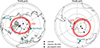 |
Figure 1 Auroral zones for the year 2020 AD, indicated by the shaded areas. Also indicated are the locations of the geomagnetic poles (diamonds), the dip poles (triangles), and polar cap centroids (squares). Also reported by the figure are the locations of four high-latitude cities considered in this study. |
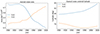 |
Figure 2 Temporal evolution of the auroral zones surface area (left) and of their centroid’s latitudes (right). The latter are reported as unsigned values, and the geographical poles are located at a latitude of 90°, for both hemispheres. As noted in Zossi et al. (2020), the evolution of the surface areas is not equatorially symmetric. |
Our calculations qualitatively agree with those reported by Zossi et al. (2020), though they differ both in the size of the auroral zone areas and in their time-dependence prior to 1940 AD. We attribute these differences primarily to the different descriptions of the polar caps, which, in Zossi et al. (2020), are defined as the areas, at Earth’s surface, enclosed by the boundary between closed and open magnetic field lines. The latter are defined, in Zossi et al. (2020), as those lines that, at their apex, reach a value of less than 49 nT, estimated to be the magnetic intensity at the magnetopause during quiet solar conditions. Note that a more rigorous definition of open magnetic field lines arises considering the magnetic reconnection between the geomagnetic field and a southward interplanetary magnetic field (Hill & Rassbach, 1975; Zossi et al., 2018).
2.2 Green’s function formalism
We now describe how we quantify the sensitivity of the auroral zones’ shape and location to changes in the main field on the CMB. Although these nonlinear diagnostics are functions of the field on the CMB, they are not given by analytic formulae, but rather a numerical recipe involving field line tracing. The standard method for quantifying geomagnetic Green’s functions for other nonlinear quantities such as the declination and inclination (Gubbins & Roberts, 1983; Johnson & Constable, 1997) does not apply here, as it relies on the quantity of interest being defined as a closed-form analytic expression of the radial magnetic field at r = re.
In order to introduce the new methodology, we apply it to the case of the radial field component Be, at Earth’s surface, for which the Green’s function is known and can be expressed as (Constable et al., 1993):
![Mathematical equation: $$ {B}_e=\frac{1}{4\pi }{\oint }_{\mathrm{CMB}} \left[\frac{{\rho }^2(1-{\rho }^2)}{{R}^3}-{\rho }^2\right]{B}_c\mathrm{d}\mathrm{\Omega }, $$](/articles/swsc/full_html/2025/01/swsc240090/swsc240090-eq15.gif) (5)
(5)
where ρ = rc/re and  , with
  the unit vector in the direction of the measurement location and
  the unit vector spanning the surface of the CMB in the above integral.
We proceed by implementing a numerical functional differentiation to construct the Green’s function, ∂Be/∂Bc. To do this, we need to choose a functional perturbation to Bc, in order to quantify the associated changes in Be. A natural approach is based on spherical harmonics because this is a common representation of the magnetic field itself. Thus, we consider functional changes to Bc and Be by changing the Gauss coefficients  in equation (3), up to degree L, making use of the shorthand notation
  to indicate either
  or
or  at a given epoch. By making use of the chain rule for derivatives, the sensitivity with respect to Bc can then be expressed as:
 (6)
(6)
In the above,  , a standard partial derivative, is the sensitivity of Be with respect to the Gauss coefficient
  , while
  , a functional derivative, is the sensitivity of the Gauss coefficients with respect to the CMB radial field. Because the radial field can be written in terms of spherical harmonics from equation (3):
 (7)
(7)
it follows that the Gauss coefficients can be written as
 (8)
(8)
where  are the Schmidt quasi-normalised spherical harmonics, representing either
  or
or  , with norm (see e.g., Backus et al., 1996):
and the integration is performed over the surface of the sphere at radius r. Taking the functional derivative in Br(r, θ, ϕ) of equation (8):
 (9)
(9)
In expressions (8) and (9), we explicitly indicated the functional dependence of Br on the spatial coordinates. By setting r = rc in the above formula, we obtain the functional derivative needed in (6). The derivative  can be computed directly from (7):
 (10)
(10)
Thus a truncated form of the analytic Green’s function can be written:
The equivalency of the above expression with (5) is shown in the Appendix of Constable et al. (1993).
In this study, we are interested in scalar diagnostics, Q, that are non-linear and non-analytic functions of Bc and hence of  . Generalising equation (10), the Green’s functions of interest can then be written:
 (11)
(11)
where  is the sensitivity of the Gauss coefficients with respect to the radial field (usually to be taken on the CMB, but it could also be on the Earth’s surface), given by (9). In place of the analytic derivative for
  we adopt a numerical forward-difference approximation. For each Gauss coefficient
  , we impose a variation
  and so obtain a perturbed quantity Q+. The difference in the observable caused by the perturbation
  is written as:
 (12)
(12)
The required derivative is estimated by dividing δQ by  :
:
 (13)
(13)
The above relationship is approximately an equality for  small enough so that the variations of Q with
  can be considered linear (for more details, see Sect. 3.1 and the discussion in Supplementary Material).
One of the goals of the present study is to relate temporal changes in the geomagnetic field with temporal changes in observables related to the auroral zones geometry and locations. The temporal variation of the Gauss coefficients can be obtained from geomagnetic field models. Another application of the chain rule allows us to obtain:
 (14)
(14)
which is the change in time of Q caused by a temporal change in a specific coefficient  . The contribution of each spherical harmonic degree l to the temporal changes of Q can be calculated by summation over spherical harmonic order:
 (15)
(15)
where the above is independent of the geographical location. Similarly, the contribution to temporal changes of Q coming from temporal changes in Br at either the CMB or Earth’s surface, can be obtained via:
 (16)
(16)
Note that in expressions (15) and (16), we explicitly indicate the dependence on either the spherical harmonic degree l or the location (θ, ϕ) on the spherical surface of radius r, respectively. We also make use of the azimuthal integral of (16), denoted by an overline:
 (17)
(17)
which represents the contribution to temporal change in Q caused by the cumulative SV from a specific co-latitude, θ.
The reference geomagnetic field configuration for which the unperturbed zones are computed is given by IGRF-13 at epoch 2020. The calculation of the Green’s functions  is performed in double precision with a program we have written in Python (version 3.8.5). In formulas (14)–(16), the quantities
  , ∂Bc/∂t have been calculated via a formula equivalent to (4), using the IGRF-13 coefficients in 2015 AD and 2020 AD. The azimuthal integration in (17) has been performed, numerically, via a trapezoidal integration rule.
To test our methodology, we first considered the magnetic inclination at Leeds (at Earth’s surface) and calculated the sensitivity to changes in the Gauss coefficients and in the radial magnetic field at both the CMB and Earth’s surface. The results, illustrated in Appendix B, are in excellent agreement with both theoretical calculations and previously published results (Johnson & Constable, 1997).
Given our definition of the auroral zones as being the regions, at Earth’s surface, lying between 65° and 70° of AACGM latitude, we apply the same technique to the auroral zones surface area (indicated as Ai, where i = N, S for the northern and southern zones, respectively), the latitude of the centroids (indicated as  , where i = N, S for the northern and southern zone, respectively) and to the angular distance between the equator-ward edge of the auroral zones and selected cities: Leeds, Edmonton, Salekhard, and Dunedin. These locations have been reported in Figure 1. The geomagnetic latitudes of these cities is either approximately equal to or greater than 50 degrees and therefore highly exposed to the impact of severe space weather events (Thomson et al., 2011; Maffei et al., 2023). We indicate the great-circle angular distance of each of the selected cities from the closest auroral zone as dj, where j indicates a specific location. The distance of the auroral zones with respect to a given city is calculated by considering the auroral zone in the same hemisphere as the city and calculating the angular distance between the city and the equator-ward boundary point that is closest. This quantity is of interest for two reasons. Firstly, it is a proxy for the shape of the auroral zones and is sensitive to deformations of the auroral zones in a way that the total surface area is not. Alternative proxies for the shape have been considered in the literature (e.g., Xiong & Lühr, 2014) but they assume that the auroral zones boundaries can be parameterised as ellipses, which is an oversimplification (see Fig. 1). Secondly, our previous study (Maffei et al., 2023) has considered the evolution of the quantity dj over the current and next centuries and found much larger changes for Salekhard and Edmonton than for Leeds and Dunedin. Since all these locations are exposed to severe space weather hazard, it is of interest to further explore the dependence of changes in dj as a function of Gauss coefficients and radial magnetic field changes in more detail.
To summarize our methodology, we first estimate the Green’s function with respect to the Gauss coefficients according to equation (13), replacing Q with either Ai,  or dj. The Green’s function with respect to the CMB radial magnetic field is then estimated via (11). Having obtained these sensitivity kernels, we estimate sources of temporal changes of the quantity of interest both as a function of the spherical harmonic degree l (via Eq. (15)) and as a function of the location on the CMB (via Eq. (16)). The latter can be integrated into longitude (see Eq. (17)) to estimate the latitudinal distribution, at the CMB, of the sources of temporal changes for Ai,
  or dj.
Concerning the numerical calculation of the Green’s functions for Ai,  or dj, defined according to (13), we found that as l and m increase, a larger
  needs to be imposed to have a quantifiable change in the quantities here considered and a numerically converged Green’s function estimation. This is due to a general decrease in sensitivity to the Gauss coefficients as l and m increase. In particular, as m increases, spherical harmonic contributions become focussed in the low-latitude regions, with little effect at high latitudes, which in turn causes a decrease in the magnitude of the Green’s functions themselves. These issues, particularly pronounced for l > 5, lead to a contrast between needing to choose a large
  and the fundamental linearisation assumption behind the Green’s function approach, requires “small” perturbations. Experimentally, we found that an l-dependent variation of magnitude
  nT is generally a good compromise to obtain numerically stable results for which the Green’s functions (13) are independent of
  to 4 significant figures. Note that these values of
  are different from those adopted in Appendix B (formula (24)). In fact, when Q is the magnetic inclination, a simpler l-dependence was found to be sufficient to obtain numerically stable results. Additional details on the calculations of the Green’s functions are given in Supplementary Material.
3 Results
3.1 Sensitivity and dependence with respect to the Gauss coefficients
The auroral zone surface area Green’s functions, with respect to  , linearised around the IGRF-13 model at epoch 2020, are shown for the full main field (i.e., up to degree L = 13) in the left panels of Figure 3, for both the northern (top panels) and southern (bottom panels) auroral zones. In the right panels we report the Green’s functions linearised around a “quasi-axial dipole” field described by the axial dipole component,
  , of IGRF-13, equatorial dipole components set to
  nT and all other coefficients set to zero. We do this to emulate an axial dipole field, and the non-zero, but small,
  , and
, and  components are necessary for the aacgmv2 algorithm to calculate AACGM coordinates. The value of 0.1 nT is chosen to be the smallest, non-zero value in the IGRF-13 coefficients (e.g., the
  coefficient for 2020 AD).
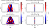 |
Figure 3 Linearised sensitivity of the auroral zones surface area change, |


To aid the reader in gaining intuition in interpreting Figure 3, some examples of how the auroral zones and their centroids vary when selected Gauss coefficients are modified are given in Supplementary Material, Figure S2 and Table S1. Restricting our attention to l ≤ 5, maximum values of sensitivity for the full IGRF-13 main field (Fig. 3, left panels) are found for l = 3, m = 0 for both the Northern and the Southern Hemisphere (with values of 355.4 km2/nT and 401.9 km2/nT, respectively). From Figure 3 (left panels) we note the decaying trend as the order m increases. This is also observed for the centroid latitudes and for the distance from selected cities (see Supplementary Material, Figs. S4 and S5). As mentioned above, this is linked to the increasingly low-latitude structure of spherical harmonics with l ≃ m, for high values of m. As a result, the changes in extension of the auroral zones are mostly insensitive to these coefficients.
As expected, the structure of  is simpler for the quasi-axial dipole field than for the full IGRF-13 field. In particular, the terms corresponding to changes in the dipolar coefficients,
  ,
,  and
and  , are all zero in the axial dipole field case, while for the full IGRF-13 field this is no longer the case. For an axial dipole background field, this is expected since a change in the dipolar coefficients alone causes a tilt of the whole field configuration, but not an increase in the area of the auroral zones (see also Supplementary Material, Fig. S4). In contrast, the more complex structure of the full field makes it possible to alter the auroral zone surface area by altering the dipole coefficients. Also from Figure 3 (left panels), we note that the signs of
  and
and  are opposite for variations in the equatorial dipole coefficients
  and
and  . Thus, the same field perturbation can have opposite effects for AN and AS.
As illustrated in Figure 2, the current trend for the auroral zone surface area is an expansion for the southern zone and a shrinking for the northern zone. As pointed out in Zossi et al. (2020) the first behaviour is in agreement with the current dipole intensity decay, while the second is due to non-trivial contribution from the non-dipolar components of the main field. To explore these behaviours more quantitatively, we computed the contributions to the yearly variation in the auroral zones surface areas from various main field components by multiplying each of the  by the SV given for the period 2015–2020 in the IGRF-13 model, according to formulas (14) and (15). In Figure 4 (left panel) we show the quantity ∂Ai/∂t, as a function of the degree l (formula (15)). The expansion of the southern auroral zone is primarily driven by l = 1 coefficients, with degrees l = 2, 3, 4 contributing to subdominant shrinking. The shrinking trend in the northern auroral zone is primarily driven by l = 2 contributions, with a subdominant (by a factor of 2) contribution from the dipolar terms. The fact that l = 1 themselves contribute to shrinking is in contradiction to the self-similar scaling laws of Siscoe & Chen (1975), Vogt & Glassmeier (2001), Glassmeier et al. (2004) and in opposition to the behaviour of the southern auroral zone. This shows the l = 1 Green’s functions already includes behaviour that cannot be expected from a purely dipolar main field. In fact, as we mentioned earlier, the
  are a function of all Gauss coefficients
  of the reference epoch for which the variations (12) are being calculated. Table 1 illustrates the calculation of ∂Ai/∂t for the dipolar SV alone. From Table 1 it is clear that the opposite sensitivities,
  , to variations in
  and
and  in the two hemispheres, are crucial in order to explain the total dipolar contribution to temporal changes in the surface area.
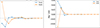 |
Figure 4 Contribution by spherical harmonic degree, l, to the change in auroral zones area (left) and centroid latitudes (right) during the period 2015–2020 AD. |
Dipole contribution to the yearly change in auroral zone surface area. The first column indicates which dipolar coefficient each row refers to. SV coefficients  are calculated as the yearly average over the 2015–2020 AD period from the IGRF-13 model, as in formula (4). The sensitivities
  are the same values as reported in Figure 3 (left panels). The temporal change contributions ∂Ai/∂t are obtained by multiplying
  with the corresponding
  . The column-wise sum of the ∂Ai/∂t values agrees with the l = 1 value reported in Figure 4 (left panel).
The result of similar calculations for changes in the centroid latitudes is shown in the right panel of Figure 4. Note that, since the latitude of the southern centroid is negative by definition, i.e.,  , Figure 4 indicates that the l = 1 SV coefficients drive both centroids to higher latitudes and closer to the geographic poles. The same remains true when one considers the total change, obtained by summing the contributions over ls, giving 0.081 deg/year for the northern centroid and −0.021 deg/year for the southern centroid. The pole-ward migration of the centroids is in agreement with the currently observed motions of the dipole axis (e.g., Alken et al., 2021). The temporal changes of the centroids latitudes are primarily driven by the dipolar SV (l = 1 Gauss coefficients), at least at present. This is expected for a dipole-dominated magnetic field. However, significant contributions from the non-dipolar components are present, in particular l = 2, and they significantly offset changes driven by the dipolar field for the southern centroid.
The contribution of each spherical harmonic degree l to temporal changes of the distance, dj, between the auroral zones and selected high-latitude cities (see Sect. 1) is shown in Figure 5. In all cases, the dominant contribution is from the l = 1 SV terms. Summing over all l we obtain dj = −0.0005, 0.008, 0.02, −0.03 deg/year for Leeds, Dunedin, Edmonton, and Salekhard, respectively; where positive values indicate that the auroral zones are moving further from the selected locations. In agreement with Maffei et al. (2023), the largest changes are obtained for Edmonton and Salekhard, since the auroral zones are currently drifting away from North America and towards Siberia. For Leeds and Dunedin, the temporal change in dj is close to zero despite a significant l = 1 contribution (see Fig. 5). As for the centroid latitudes, the dominant changes in dj are caused by changes in the dipolar components of the geomagnetic field. However, the sum of the non-dipolar contributions can be large enough to offset the dipolar one, depending on location.
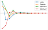 |
Figure 5 Temporal derivative of the angular distance between selected cities and the closest auroral zone for each degree l. Obtained by multiplying the kernels shown in Supplementary Figure S5 by the SV for 2020 from IGRF-13 calculated via first differences. |
Overall, our results indicate that, although a significant contribution to the evolution of the auroral zones is indeed caused by dipolar field coefficients, non-dipolar contributions can either be individually dominant (as is the case for the northern zone surface area, see Fig. 4) or combine so as to offset the dipole-driven changes (e.g., the auroral zone distance from Leeds, Fig. 5).
3.2 Sensitivity and dependence with respect to the radial magnetic field
We now turn our attention to the sensitivity of the auroral zones to geographical changes in the CMB radial magnetic field, Bc; the relevant Green’s functions are computed using formula (11). The sensitivities of the auroral zones’ surface area and centroid latitude with respect to changes in Bc, are shown in Figure 6. These figures show that the auroral zones are sensitive to changes in Bc everywhere on the CMB, and not only in the high-latitude regions.
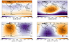 |
Figure 6 Green’s functions for the auroral zones surface area (top) and centroid latitude (bottom) with respect to changes of the radial magnetic field, Bc at the core-mantle boundary (CMB). The panels on, respectively, the left (right) refers to the northern (southern) zone. The shape of the auroral zone under consideration (northern or southern) is indicated via the red dashed lines while the location of the centroid is shown in the maps via a red square. |
The Green’s functions for the surface area (top panels of Fig. 6), referred to as ∂Ai/∂Bc, indicates that a positive increase in Bc in the high-latitude regions of the CMB causes an expansion of the northern auroral zone and a shrinking of the southern zone. A global decrease of the dipole field intensity would cause positive changes in Bc in the Northern Hemisphere and negative changes in the Southern Hemisphere, with consequent expansion of both auroral zones. This confirms that the decay of the dipole field alone is not sufficient to explain the currently observed surface area changes (see Fig. 2). The top panels of Figure 6 also show a region of opposite, although weaker, contribution from the mid-to-low latitude regions below the Atlantic Ocean. The Atlantic Hemisphere is home to intense non-dipolar SV features (e.g., Finlay et al., 2020) and the mid-to-low latitude features of ∂Ai/∂Bc suggest, in agreement with Figure 4, that non-dipolar SV contributes significantly to the observed changes in surface area of the auroral zones, even though the sensitivity to changes in the region is weaker than at higher latitudes.
The Green’s functions  for the centroids latitude with respect to the CMB radial fields are shown in the bottom panels of Figure 6. Their structure indicates a high sensitivity to changes in the equatorial dipole field components. Sensitivity to non-dipolar contributions are evident in the location of the maxima, located northward of the equator for the northern centroid, and southward for the southern centroid.
Figure 7 illustrates the geographical contribution of  (estimated via formula (4)) to the changes in surface areas ∂Ai/∂t(θ, ϕ) and centroid latitudes
  , between 2015 and 2020 AD. These have been obtained from the appropriate versions of the formula (16). The rightmost panels in Figure 7 show the azimuthally integrated contribution (Eq. (17)). Considering the surface area changes first (top panel of Fig. 7), these figures illustrate non-trivial positive and negative contributions from different regions of the CMB. In particular, note the positive and negative patches on the CMB underneath the low-latitude Atlantic Ocean and southern Africa, particularly in the southern auroral zone (Fig. 7, top-middle panel). As mentioned above, these patches emerge in spite of the subdominant sensitivity in the region (see Fig. 6) because of the strong SV there. Without our analysis, it is not obvious whether these regions have a net impact on the surface area changes of the auroral zones. To explore their contribution more quantitatively, we show, in the top-right panel of Figure 7 the azimuthal integral of ∂Ai/∂t(θ, ϕ). This quantity has been obtained via formula (17) with the purpose of isolating the latitudinal contribution. Low-latitude, non-negligible CMB contributions to the change of auroral zones surface area clearly emerges from Figure 7. For the northern zone, the main negative contributions (leading to the observed shrinking) peak around 75° and
  latitude, both of the same order of magnitude (between 104 and 2 · 104 km2/year). A positive peak of similar magnitude can be seen around 60° of latitude and multiple subdominant contributions are present at all latitudes. We also note that the net contribution of the strong polar patches largely cancels out at latitudes above 75°. For the southern auroral zone the main positive contribution (in line with the observed expansion) is located near the equator, and secondary peaks are visible at high latitudes in both hemispheres. We can therefore conclude that the observed evolution of the auroral zone surface areas are not solely driven by high-latitude magnetic field variations, and that the entire CMB, including the low-latitude regions, plays an important role in setting the observed evolution, especially for the southern auroral zone.
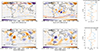 |
Figure 7 CMB sources of changes in the auroral zone surface area (top panels) and centroid latitude (bottom panels), during the period 2015–2020 AD. Results for the northern and southern zones are shown, respectively, in the left and middle panels. The rightmost panel illustrates the azimuthally integrated contribution (Eq. (17)). |
The total surface area change predicted between 2015 and 2020 AD can be obtained by integrating ∂Ai/∂t(θ, ϕ) over the entire CMB. In performing this calculation, the latitudinal integration has been implemented via the Gauss-Legendre quadrature (Olver et al., 2010, Chapter 3.5(v)). The resulting estimate is compared, in Table 2, with the first-differences variation obtained directly from 2015 and 2020 results shown in Figure 2.
Changes in auroral zones surface area, AN (first row) and AS (second row), between 2015 and 2020 AD. The second column reports the first-difference estimate from Ai calculated using the IGRF-13 model (analogous to formula (4)). The third column reports the estimates obtained by integrating geographical sources of change over the CMB (top panels of Fig. 7).
As for the magnetic inclination example reported in Appendix B (see Table B1), the Green’s function estimate is in approximate agreement with the direct first-difference calculation, the differences being due to linearisation.
Changes of magnetic inclination, I, at Leeds, between 2015 and 2020 AD. The first row reports the first-difference estimate from the IGRF-13 model (analogous to formula (4)). The second row reports an estimate obtained by linearising ∂I/∂t in changes in surface magnetic field (similar to Eq. B2). The third and fourth rows show the estimates obtained by integrating geographical sources of change over the CMB and Earth’s surface, respectively (i.e., Eq. (16)).
From the bottom panels of Figure 7, we see that, as expected from the analysis of Figure 6, most of the sources of the centroid’s latitude change are concentrated in the middle- to low-latitudes (including the SAA region). Furthermore, we note that  , which follows from the shape of the Green’s functions with respect to Bc (Fig. 6). Remarkably, this results in both centroids latitude being almost unaffected by the CMB SV at high, northern latitudes. The northern zone centroid latitude is therefore, at present, very weakly controlled by the CMB field at high latitudes in the same hemisphere.
The sensitivity of dj (the distance between a selected location and the nearest auroral zone) to changes in Bc and its CMB sources of temporal changes are given, respectively, in Figures 8 and 9. These are calculated in a similar fashion as the results reported in Figures 6 and 7. Figure 8 illustrates how changes in the radial magnetic field at the CMB, locally stretch or compress the auroral zones at particular locations. This sensitivity is largest for wide regions equator-ward of the point on the CMB directly beneath the locations, with opposite sensitivity at antipodal locations. This latter observation suggests that an overall tilt of the radial magnetic field at the CMB, rather than localised, regional changes, are the most efficient way of modifying the quantity dj, in agreement with the overall dominance of the l = 1 contribution in Figure 5. The qualitative similarity between the Green’s functions ∂dj/∂Bc for Leeds and Dunedin explains the similarities of the resulting source of temporal changes ∂dj/∂t shown in Figure 7. This is due to the near-antipodal location of the two cities and therefore an overall tilt of the dipole in a certain direction would, at least for a purely dipolar magnetic field, influence their dj by the same amount.
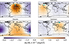 |
Figure 8 Green’s function for the angular distance between selected cities and the closest auroral zone with respect to the radial field at the CMB. The selected location is shown on the maps as a cyan dot. |
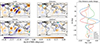 |
Figure 9 CMB sources of temporal changes in the auroral zone angular distance from selected cities, during the period 2015–2020 AD. The rightmost panel illustrates the azimuthally integrated contribution (Eq. (17)). The selected locations are shown on the maps as cyan dots. |
The smaller magnitudes of both ∂dj/∂Bc (Fig. 8) and ∂dj/∂t (see the maps of Fig. 9), for Edmonton and Salekhard, are primarily caused by the different magnitude of the sensitivity to changes in  . The latter is larger, in magnitude, for Leeds and Dunedin, while the sensitivity to changes in
  and
and  is of comparable magnitude for all cities.
Overall, Figure 9 shows that the temporal changes in dj are not primarily driven by polar Bc as there are also strong contributions from SV at lower latitudes. Despite the larger magnitudes of CMB contributions for Leeds and Dunedin, the total change, ∂dj/∂t, in the period 2015–2020 AD, is much smaller than for Edomonton and Salekhard (see Sect. 3.1). This is due to non-trivial cancellations of the CMB contributions, and, for the Northern Hemisphere, it is in line with the overall translation of the northern auroral zone in the direction of Siberia (e.g., Maffei et al., 2023). We explore this aspect in more detail in the next section.
3.3 Effect of individual SV components
In order to further interpret the results presented above, we illustrate, in Figure 10, the effect that the SV components l = 1, 2, 3 have on changes of the shape and position of the auroral zones.
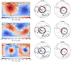 |
Figure 10 Effect of l = 1, 2, 3 components (respectively top, middle, and bottom panels) of the SV on the shape and position of the auroral zones. For illustrative purposes, the actual SV has been magnified by a factor of 100. Left panels: the magnified SV components at the CMB. Middle and right panels: the northern and auroral zones, plotted with the centroid positions for the 2020 IGRF-13 model (red) and the same model, on top of which the SV shown in the left panels is added (blue). |
These degrees have been selected for closer inspection as they have been found to be the major contributors to total changes in the diagnostics we have considered (see Figs. 4 and 5). In Table 3, we report the relative change in surface area, and distance between the auroral zones and Leeds and Dunedin, difficult to discern from an inspection of Figure 10 alone.
Relative changes in auroral zones surface areas, and distances from Leeds and Dunedin, caused by l = 1, 2, 3 components of the SV, magnified by a factor of 100 (indicated in the table). The reported values are obtained as the changes relative to the unperturbed 2020 auroral zones, calculated from the IGRF-13 model. These values refer to the results shown in Figure 10 and have been reported in the table for ease of quantitative comparison.
Since the actual SV produces, for the annual-to-interannual periods here considered, auroral zone changes that are difficult to discern by eye, we multiplied the SV components by a factor of 100. Within the framework of linearised changes, this shows the possible changes over 100 years of constant SV. The resulting SV produces changes that violate the small-perturbation approximation needed to meaningfully calculate Green’s functions. Nevertheless, these examples show how the low-degree SV components drive changes that are qualitatively in agreement with the results shown earlier and with findings on multi-decadal timescales (Maffei et al., 2023). In particular, we see, from Figure 10 and Table 3, that the dipolar, l = 1, SV produces opposite changes in the northern and southern zones surface area, in agreement with Figure 4. The changes in the centroid latitudes and overall zone positions are most efficiently driven by the l = 1 SV. The degrees l = 2, 3 impart modifications that are crucial in explaining the changes caused by the total SV. Namely, the dipolar SV causes the distance between Leeds and the northern zone increase, while the higher degrees compensate for this effect, in agreement with Figure 5. This cancelation explains the small change caused by the total SV found above and in Maffei et al. (2023). Similarly, we see that each degree causes significant alterations in the shape and location of the southern auroral zone, but their effects combine to produce small changes even on multi-decadal timescales Maffei et al. (2023).
The low-degree SV considered in the left panels of Figure 10 dominates the changes in the auroral zones and has a markedly global structure. In particular, there is a strong sensitivity at mid-to-low latitude regions, in agreement with the results of Figures 7 and 9. When individual SV components are evaluated at Earth’s surface their magnitude is scaled by a factor of (rc/ra)(l+1) (see Eq. (3)) but their pattern remains unchanged. We can therefore conclude that the evolution of the auroral zones would similarly be reflected in low-latitude surface SV features.
4 Conclusions
Our main conclusion is that the auroral zones’ temporal changes depend on the global structure of SV at the CMB. They cannot be solely described by the dipolar contribution to the secular variation, nor by only the high-latitude geomagnetic field changes. Although these approximations result in simple models (e.g., Korte & Stolze, 2016) and physical insights (e.g., Zossi et al., 2020) of auroral zones evolution, important features might be lost when the full spatial complexity of the main geomagnetic field is not considered.
In order to explore these issues, we introduced a novel methodology to link the temporal evolution of the auroral zones with temporal changes of the main magnetic field. Our methodology is based upon a Green’s function formalism that allows us to link the sensitivity of the auroral zones’ shape and location with changes in the Gauss coefficients that describes the geomagnetic SV. No assumption was made concerning the shape of the main field or of the auroral zones. The former was taken from IGRF-13 (Alken et al., 2021), which contains a time-dependent description of both dipolar and non-dipolar Gauss coefficients, up to degree l = 13. The recent spatiotemporal features captured by this model are heavily constrained by the data provided by ESA’s Swarm geomagnetic mission. The auroral zones were obtained by calculating AACGM latitudes via a methodology that considers all given Gauss coefficients (Shepherd, 2014), and without parameterising the boundaries of the auroral zones as, say, circles or ellipses (e.g., Korte & Stolze, 2016; Xiong & Lühr, 2014). Our methodology is therefore capable of describing the shape of the auroral zones in their full generality.
In the present study we focussed on key diagnostic quantities that characterise the extension, shape and location of the auroral zones: their surface area, the location of their geometrical center (i.e., their centroid), and the angular distance between selected, mid-to-high latitude cities and the equator-ward edge of the closest auroral zone. Sensitivity of these quantities to the geomagnetic Gauss coefficients have been obtained numerically by perturbing the IGRF-13 model (see Eq. (13)). From these sensitivity kernels, we obtained the linearised sensitivities to changes in CMB radial magnetic field (via Eq. (11)) and the sources of temporal changes for all diagnostics as a function of Gauss coefficients order (via Eq. (15)) and CMB location (via Eq. (16)).
We found that non-dipolar contributions, up to about l = 5, significantly affect the evolution of the auroral zones (see Figs. 4 and 5), and that the non-dipolar nature of the geomagnetic field is the largest contributor of temporal changes of specific auroral zone features. This is the case, for example, for the observed shrinking of the northern auroral zone (see Fig. 4 and Zossi et al., 2020, 2021), which cannot be explained by known scaling laws (Siscoe & Chen, 1975; Cnossen et al., 2012) that assume a purely dipolar control of the magnetosphere’s shape; the full structure of the main field must be taken into account. Even when our analysis revealed a large dipolar contribution, non-dipolar terms can completely offset the leading order behaviour. This has been observed for the evolution of the distance between the northern auroral zone and Leeds, a proxy for the deformation or motion of the auroral zone along, approximately, the Greenwich meridian direction at 0° longitude.
We also found that the auroral zone temporal evolution significantly controlled by the geomagnetic field variations at low and mid latitudes (see Figs. 6–8 and 10). The high-latitude SV at the CMB can have a net contribution that is either intrinsically small or large but completely opposed by SV at low latitudes. Interpreting changes in the auroral zone shape and location solely in terms of polar field changes at the CMB can therefore be misleading.
Our results indicate that the auroral zones are currently highly sensitive to changes of the main field in the mid-to-low latitude regions, particularly on the CMB under the Atlantic. This area is known to be characterised by high levels of SV and contains geomagnetic features that result in the SAA (see Finlay et al., 2020 and references therein). Since the low magnetic field intensity of the SAA favours the occurrence of equatorial aurorae in South Atlantic regions (He et al., 2020), our result suggests an intriguing link between two seemingly unrelated regions capable of visible auroral activity. The SAA is currently expanding, shifting westward and splitting into two main minima (Terra-Nova et al., 2019). This complex temporal evolution may have non-trivial, future consequences on the shape and locations of the auroral zones.
Acknowledgments
The authors are grateful to Joseph W. B. Eggington, Jonathan P. Eastwood (Imperial College London), Sabrina Sanchez (IPGP Paris) and Mervyn P. Freeman (British Antarctic Survey, Cambridge) for invaluable suggestions and fruitful discussions on many of the topics dealt with in the present study. The editor thanks two anonymous reviewers for their assistance in evaluating this paper.
Funding
This research was funded by NERC Grant Number NE/P016758/1 (S.M., P.W.L and J.E.M.). S.M. also acknowledges funding contributions from the European Research Council (agreement 833848-UEMHP) under the Horizon 2020 programme.
Data availability statement
Numerical values of the Green’s function, from which the results are shown in the present paper can be derived, can be found at the Github repository https://github.com/smaffei/auroral_forecast.git. In the same repository, scripts to reproduce the figures reported in this paper are made available.
Supplemetary material
Supplementary file: Sensitivity of the auroral zones to temporal changes in earth’s internal magnetic field: Supporting information. Access Supplementary Material
Appendix A
The geometric center of a spherical polygon
In this Appendix, we give the formula used to calculate the location of the centroids of the auroral zones. These are defined as the geometric centers (or centers of mass) of the polar caps, the areas enclosed by the poleward boundaries of the auroral zones.
Numerically speaking, the polar cap boundary is a closed polygon on the surface of Earth, assumed to be a spherical surface of radius re and center O. The polygon representing the polar cap boundary is composed of N vertices, with the ith vertex denoted by Pi. We enumerate the vertices from i = 1 to i = N. The vertices are connected by great-circle segments and the angle between the two segments connecting at the point Pi is denoted with 
Let vi the vector that originates in O and ends on the vertex Pi (pointing outwards). Extending Brock (1975), we define the location of the geometric center of the polygon as:
where A is the surface area enclosed by the polygon and it is assumed that v1 = vN+1. Note that, in order for the above formula to refer to the correct surface, the path identified by the succession of vertices P1, P2, … PN has to be traversed so that the area of interest is to the left of the path.
By definition, the centroid is defined via the moment of inertia, M, of the surface such as:

from which it follows that:
Furthermore, since the polar cap centroid lies on the surface of the sphere, the norm of the vector c is |c| = re. This leads to the final formula:

In practice the above calculation is performed in cartesian coordinates. The final result is then converted in spherical coordinates so that the centroid latitude,  , is obtained.
Appendix B
Proof-of-concept: magnetic inclination at Leeds
In order to test our methodology, we calculated the Green’s function of the magnetic inclination with respect to  and to the CMB radial field Bc. The magnetic inclination, I, (or briefly, inclination) is defined as, at a specific location at the Earth’s surface:
 (B1)
(B1)
where  is the horizontal field intensity (at Earth’s sruface) and the components of the magnetic field (Be, Bθ, Bϕ) can be obtained from (3). The variations of I with respect to the Gauss coefficient
  , which we refer to as
  are calculated differentiating equation (B1):
 (B2)
(B2)
where  is the total field intensity at Earth’s surface. Since B is a linear function of the Gauss coefficients, the Green’s functions of the magnetic field components with respect to
  can be readily derived from (3):
 (B3)
(B3)
 (B4)
(B4)
 (B5)
(B5)
We therefore have a closed-form, analytical solution for the Green’s function of the magnetic inclination with respect to the Gauss coefficients (B2).
This solution is illustrated in Figure B1 (top-left panel, black crosses) for the location of Leeds (latitude λ = 53.81° North and longitude ϕ = 1.549° West) and for a background field given by the IGRF-13 model in 2020. Numerical solutions for  are calculated, for the same location, by explicitly calculating
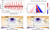 |
Figure B1 Green’s function for the magnetic inclination with respect to the Gauss coefficients (top-left panel) compared to their theoretical expectation. On the horizontal axis, the Gauss coefficients are grouped according to their degree l and ordered as: |
 (B6)
(B6)
where I is the unperturbed inclination and I+ is the inclination obtained by augmenting the coefficient  by a perturbation
  . The perturbations were chosen small enough so that I+ − I is linear in
  . It was empirically found that:
 (B7)
(B7)
gave excellent agreement with the analytical solution (B2). Figure B1 (top-right panel) shows the numerical solution in matrix form, highlighting the sensitivity to  and
and  . The sensitivity of the inclination with respect to the
  coefficients is much smaller than the sensitivity with respect to
  , due to the reference location, very close to the ϕ = 0 meridian.
From the sensitivity to the Gauss coefficients it is possible to calculate the sensitivity to unit changes of the radial magnetic field at the CMB, ∂I/∂Bc, via a formula analogous to (11):
In Figure B1 (bottom-left panel), we illustrate the result obtained for the 2020 epoch taken from the IGRF-13 model at Leeds, the location of which is marked by the yellow star in Figure B1. Figure B1 is visually indistinguishable from Green’s function calculated according to the formula reported in Johnson & Constable (1997):
![Mathematical equation: $$ \frac{{\partial I}}{\partial {B}_c}=\frac{1}{{H}^2+{Z}^2}\left[H{\mathcal{G}}_Z-\frac{Z}{H}(X{\mathcal{G}}_X+Y{\mathcal{G}}_Y)\right], $$](/articles/swsc/full_html/2025/01/swsc240090/swsc240090-eq122.gif)
with (Constable et al., 1993):
![Mathematical equation: $$ \begin{array}{ll}{\mathcal{G}}_X& =-\frac{1}{4\pi }\frac{1+2R-{\rho }^2}{{R}^3T}{\rho }^3\widehat{\mathbf{s}}\cdot \widehat{\mathbf{x}},\\ {\mathcal{G}}_Y& =-\frac{1}{4\pi }\frac{1+2R-{\rho }^2}{{R}^3T}{\rho }^3\widehat{\mathbf{s}}\cdot \widehat{\mathbf{y}},\\ {\mathcal{G}}_Z& =\frac{1}{4\pi }\left[{\rho }^2-\frac{{\rho }^2(1-{\rho }^2)}{{R}^3}\right],\end{array} $$](/articles/swsc/full_html/2025/01/swsc240090/swsc240090-eq123.gif)
and shown in Figure B1, bottom-right panel. In the above X, Y, and Z are, respectively, North, East and downward pointing magnetic field components at Earth’s surface ρ = rc/re,  , T = 1 + R − μρ and
  , where
  is the unit vector in the direction of the observation location on Earth’s surface,
  is a unit vector spanning the CMB, and
  and
and  are the Northward and Eastward unit vectors at the observation location.
Figure B1 illustrates the inclination at the Earth’s surface is sensitive to both changes in the radial magnetic field in the vicinity of the projection on the CMB of the observation location, and to changes at remote locations, in particular in regions close to the North Pole.
To estimate the total change of inclination between 2015 and 2020 AD, we follow formula (16) and multiply the sensitivity to the radial field, ∂I/∂Br (at either the CMB or Earth’s surface) with the actual temporal variation obtained from the IGRF-13 model via first-differences (see definition (4)). The result, integrated over the spherical surface, is reported in the last two rows of Table B1 for, respectively, the changes at the CMB, (∂I/∂t)GC, and at Earth’s surface, (∂I/∂t)GE. Numerically, the latitudinal integral is calculated via the Gauss-Legendre quadrature (Olver et al., 2010, Chapter 3.5(v)). As expected, and to confirm the validity of our numerical procedure, the two estimates agree with each other. These Green’s function estimates can be compared with the actual change of inclination,  , during the 2015–2020 period (first row of Table B1) and with an estimate, (∂I/∂t)LB, obtained by linearising ∂I/∂t in the temporal variation of the magnetic field components (second row of Table B1). As expected from the linear nature of the Green’s function approach, (∂I/∂t)GC and (∂I/∂t)GE agree with the linear estimate (∂I/∂t)LB, and not with the variation
  itself. The difference between the linear estimates and
  is, in this particular case, around 50%.
References
- Akasofu S-I. 1983. Evolution of ideas in solar-terrestrial physics. Geophys J Int 74(1): 257–299. https://doi.org/10.1111/j.1365-246X.1983.tb01880.x. [Google Scholar]
- Alexeev II. 2005. What defines the polar cap and auroral oval diameters? In: The inner magnetosphere: physics and modeling, Pulkkinen TI, Tsyganenko NA, Friedel RHW (Eds), American Geophysical Union, pp. 257–262. ISBN 9781118666098. https://doi.org/10.1029/155GM27. [Google Scholar]
- Alken P, Thébault E, Beggan CD, Amit H, Aubert J, et al. 2021. International geomagnetic reference field: the thirteenth generation. Earth Planets Space 73(1): 49. https://doi.org/10.1186/s40623-020-01288-x. [NASA ADS] [CrossRef] [Google Scholar]
- Backus G, George B, Parker RL, Parker R, Constable C. 1996. Foundations of geomagnetism. Cambridge University Press. ISBN 9780521410069. [Google Scholar]
- Baker KB, Wing S 1989. A new magnetic coordinate system for conjugate studies at high latitudes. J Geophys Res Space Phys 94(A7): 9139–9143. https://doi.org/10.1029/JA094iA07p09139. [Google Scholar]
- Bevis M, Cambareri G. 1987. Computing the area of a spherical polygon of arbitrary shape. Math Geol 19(4): 335–346. https://doi.org/10.1007/BF00897843. [Google Scholar]
- Blake SP, Pulkkinen A, Schuck PW, Glocer A, Tóth G. 2021. Estimating maximum extent of auroral equatorward boundary using historical and simulated surface magnetic field data. J Geophys Res Space Phys 126(2): e2020JA028284. https://doi.org/10.1029/2020JA028284. [Google Scholar]
- Brock JE. 1975. The inertia tensor for a spherical triangle. J Appl Mech 42(1): 239–239. https://doi.org/10.1115/1.3423535. [Google Scholar]
- Cnossen I, Richmond AD, Wiltberger M. 2012. The dependence of the coupled magnetosphere-ionosphere-thermosphere system on the Earth’s magnetic dipole moment. J Geophys Res Space Phys 117(A5): A05302. https://doi.org/10.1029/2012JA017555. [Google Scholar]
- Constable C, Constable S. 2023. A grand spectrum of the geomagnetic field. Phys Earth Planet Inter 344: 107090. https://doi.org/10.1016/j.pepi.2023.107090. [Google Scholar]
- Constable CG, Parker RL, Stark PB. 1993. Geomagnetic field models incorporating frozen-flux constraints. Geophys J Int 113(2): 419–433. https://doi.org/10.1111/j.1365-246X.1993.tb00897.x. [Google Scholar]
- Dungey JW. 1961. Interplanetary magnetic field and the auroral zones. Phys Rev Lett 6: 47–48. https://doi.org/10.1103/PhysRevLett.6.47. [CrossRef] [Google Scholar]
- Feldstein Y. 2016. The discovery and the first studies of the auroral oval: a review. Geomagn Aeron 56(2): 129–142. https://doi.org/10.1134/S0016793216020043. [Google Scholar]
- Feldstein Y, Starkov G. 1970. The auroral oval and the boundary of closed field lines of geomagnetic field. Planet Space Sci 18(4): 501–508. https://doi.org/10.1016/0032-0633(70)90127-3. [Google Scholar]
- Feldstein YI. 1986. A quarter of a century with the auroral oval. Eos Trans Am Geophys Union 67(40): 761–767. https://doi.org/10.1029/EO067i040p00761-02. [Google Scholar]
- Finlay CC, Kloss C, Olsen N, Hammer MD, Tøffner-Clausen L, Grayver A, Kuvshinov A. 2020. The CHAOS-7 geomagnetic field model and observed changes in the South Atlantic Anomaly. Earth Planets Space 72(1): 1–31. https://doi.org/10.1186/s40623-020-01252-9. [NASA ADS] [CrossRef] [Google Scholar]
- Giaquinta M, Hildebrandt S. 2004. Calculus of Variations I. Grundlehren der mathematischen Wissenschaften. Springer Berlin Heidelberg, ISBN 9783540506256. [Google Scholar]
- Glassmeier K-H, Vogt J, Stadelmann A, Buchert S. 2004. Concerning long-term geomagnetic variations and space climatology. Ann Geophys 22(10): 3669–3677. https://doi.org/10.5194/angeo-22-3669-2004. [Google Scholar]
- Gubbins D, Jones AL, Finlay CC. 2006. Fall in Earth’s magnetic field is erratic. Science 312(5775): 900–902. https://doi.org/10.1126/science.1124855. [Google Scholar]
- Gubbins D, Roberts N. 1983. Use of the frozen flux approximation in the interpretation of archaeomagnetic and palaeomagnetic data. Geophys J Int 73(3): 675–687. https://doi.org/10.1111/j.1365-246X.1983.tb03339.x. [Google Scholar]
- Hammer MD, Finlay CC. 2018. Local averages of the core-mantle boundary magnetic field from satellite observations. Geophys J Int 216(3): 1901–1918. https://doi.org/10.1093/gji/ggy515. [Google Scholar]
- Hayakawa H, Tamazawa H, Ebihara Y, Miyahara H, Kawamura AD, Aoyama T, Isobe H. 2017. Records of sunspots and aurora candidates in the Chinese official histories of the Yuán and Máng dynasties during 1261–1644. Publ Astron Soc Jpn 69(4): 65. https://doi.org/10.1093/pasj/psx045. [Google Scholar]
- He F, Wei Y, Wan W. 2020. Equatorial aurora: the aurora-like airglow in the negative magnetic anomaly. Natl Sci Rev 7(10): 1606–1615. https://doi.org/10.1093/nsr/nwaa083. [Google Scholar]
- Hill TW, Rassbach ME. 1975. Interplanetary magnetic field direction and the configuration of the day side magnetosphere. J Geophys Res 80(1): 1–6. https://doi.org/10.1029/JA080i001p00001. [Google Scholar]
- Hope ER. 1957. Linear secular oscillation of the northern magnetic pole. J Geophys Res 62(1): 19–27. https://doi.org/10.1029/JZ062i001p00019. [Google Scholar]
- Jackson A, Finlay C. 2015. Geomagnetic secular variation and its applications to the core. In: Treatise on geophysics, 2nd edn, Schubert G (Ed.), Elsevier, Oxford, pp. 137–184. ISBN 978-0-444-53803-1. https://doi.org/10.1016/B978-0-444-53802-4.00099-3. [Google Scholar]
- Johnson CL, Constable CG. 1997. The time-averaged geomagnetic field: global and regional biases for 0–5 Ma. Geophys J Int 131(3): 643–666. https://doi.org/10.1111/j.1365-246X.1997.tb06604.x. [Google Scholar]
- Kataoka R, Nakano S. 2021. Auroral zone over the last 3000 years. J Space Weather Space Clim 11: 46. https://doi.org/10.1051/swsc/2021030. [Google Scholar]
- Korte M, Mandea M. 2008. Magnetic poles and dipole tilt variation over the past decades to millennia. Earth Planets Space 60(9): 937–948. https://doi.org/10.1186/BF03352849. [Google Scholar]
- Korte M, Stolze S. 2016. Variations in mid-latitude auroral activity during the holocene. Archaeometry 58(1): 159–176. https://doi.org/10.1111/arcm.12152. [Google Scholar]
- Kubo Y, Saito S, Tsugawa T, Ebihara Y, Nagatsuma T, Sato T, Jin H. 2023. Impact of space weather on various fields. In: Solar-terrestrial environmental prediction, Kusano K (Ed.), Springer Nature Singapore, Singapore, pp. 9–79. ISBN 978-981-19-7765-7. https://doi.org/10.1007/978-981-19-7765-7_2. [Google Scholar]
- Laundal KM, Richmond AD. 2017. Magnetic coordinate systems. Space Sci Rev 206(1–4): 27–59. https://doi.org/10.1007/s11214-016-0275-y. [CrossRef] [Google Scholar]
- Lesur V, Gillet N, Hammer M, Mandea M. 2022. Rapid variations of Earth’s core magnetic field. Surv Geophys 43(1): 41–69. https://doi.org/10.1007/s10712-021-09662-4. [Google Scholar]
- Livermore PW, Finlay CC, Bayliff M. 2020. Recent north magnetic pole acceleration towards Siberia caused by flux lobe elongation. Nat Geosci 13(5): 387–391. https://doi.org/10.1038/s41561-020-0570-9. [Google Scholar]
- Longden N, Chisham G, Freeman MP, Abel GA, Sotirelis T. 2010. Estimating the location of the open-closed magnetic field line boundary from auroral images. Ann Geophys 28(9): 1659–1678. https://doi.org/10.5194/angeo-28-1659-2010. [Google Scholar]
- Maffei S, Eggington JW, Livermore PW, Mound JE, Sanchez S, Eastwood JP, Freeman MP. 2023. Climatological predictions of the auroral zone locations driven by moderate and severe space weather events. Sci Rep 13(1): 779. https://doi.org/10.1038/s41598-022-25704-2. [Google Scholar]
- Mandea M, Dormy E. 2003. Asymmetric behavior of magnetic dip poles. Earth Planets Space 55(3): 153–157. https://doi.org/10.1186/BF03351742. [Google Scholar]
- Milan SE. 2009. Both solar wind-magnetosphere coupling and ring current intensity control of the size of the auroral oval. Geophys Res Lett 36(18): L18101. https://doi.org/10.1029/2009GL039997. [Google Scholar]
- Noeldeke C, Boettcher M, Mohr U, Gaisser S, Alvarez Rua M, Eickhoff J, Leslie M, Von Thun M, Klinkner S, Varatharajoo R. 2021. Single event upset investigations on the “Flying Laptop” satellite mission. Adv Space Res 67(6): 2000–2009. https://doi.org/10.1016/j.asr.2020.12.032. [Google Scholar]
- Oguti T. 1993a. The auroral zone in historic times–the Northern UK was in the auroral zone 300 years ago. J Geomag Geoelectr 45(3): 231–242. https://doi.org/10.5636/jgg.45.231. [Google Scholar]
- Oguti T. 1993b. A note on the auroral frequency charts by Ritz and Vestine. J Geomag Geoelectr 45(5): 449–454. https://doi.org/10.5636/jgg.45.449. [Google Scholar]
- Oguti T. 1993c. Prediction of the location and form of the auroral zone: wandering of the auroral zone out of high latitudes. J Geophys Res Space Phys 98(7): 11649–11655. https://doi.org/10.1029/93JA00328. [Google Scholar]
- Olsen N, Mandea M. 2007. Will the magnetic North Pole move to Siberia? Eos Trans Am Geophys Union 88(29): 293–293. https://doi.org/10.1029/2007EO290001. [Google Scholar]
- Olver F, Lozier D, Boisvert R, Clark C. 2010. The NIST handbook of mathematical functions. Cambridge University Press, New York, NY. [Google Scholar]
- Richmond A. 1995. Ionospheric electrodynamics using magnetic apex coordinates. J Geomag Geoelectr 47(2): 191–212. https://doi.org/10.5636/jgg.47.191. [CrossRef] [Google Scholar]
- Shepherd SG. 2014. Altitude-adjusted corrected geomagnetic coordinates: Definition and functional approximations. J Geophys Res Space Phys 119(9): 7501–7521. https://doi.org/10.1002/2014JA020264. [Google Scholar]
- Silverman SM. 1992. Secular variation of the aurora for the past 500 years. Rev Geophys 30(4): 333–351. https://doi.org/10.1029/92RG01571. [Google Scholar]
- Silverman SM, Hayakawa H. 2021. The Dalton minimum and John Dalton’s auroral observations. J Space Weather Space Clim 11: 17. https://doi.org/10.1051/swsc/2020082. [CrossRef] [EDP Sciences] [Google Scholar]
- Siscoe GL, Chen CK. 1975. The paleomagnetosphere. J Geophys Res 80(34): 4675–4680. https://doi.org/10.1029/JA080i034p04675. [Google Scholar]
- Terra-Nova F, Amit H, Choblet G. 2019. Preferred locations of weak surface field in numerical dynamos with heterogeneous core-mantle boundary heat flux: consequences for the South Atlantic Anomaly. Geophys J Int 217(2): 1179–1199. https://doi.org/10.1093/gji/ggy519. [Google Scholar]
- Thomson AWP, Dawson EB, Reay SJ. 2011. Quantifying extreme behavior in geomagnetic activity. Space Weather 9(10): S10001. https://doi.org/10.1029/2011SW000696. [Google Scholar]
- Tsyganenko NA. 2019. Secular drift of the auroral ovals: how fast do they actually move? Geophys Res Lett 46(6): 3017–3023. https://doi.org/10.1029/2019GL082159. [Google Scholar]
- Tsyganenko NA, Andreeva VA. 2015. A forecasting model of the magnetosphere driven by an optimal solar wind coupling function. J Geophys Res Space Phys 120(10): 8401–8425. https://doi.org/10.1002/2015JA021641. [Google Scholar]
- Van Zandt TE, Clark WL, Warnock JM. 1972. Magnetic apex coordinates: a magnetic coordinate system for the ionospheric F 2 layer. J Geophys Res 77(13): 2406–2411. https://doi.org/10.1029/JA077i013p02406. [Google Scholar]
- Vogt J, Glassmeier K-H. 2001. Modelling the paleomagnetosphere: strategy and first results. Adv Space Res 28(6): 863–868. https://doi.org/10.1016/S0273-1177(01)00504-X. [Google Scholar]
- Wagner D, Neuhäuser R. 2019. Variation of the auroral oval size and offset for different magnetic activity levels described by the Kp-index. Astron Nachr 340(6): 483–493. https://doi.org/10.1002/asna.201913601. [CrossRef] [Google Scholar]
- Xiong C, Lühr H. 2014. An empirical model of the auroral oval derived from CHAMP field-aligned current signatures – Part 2. Ann Geophys 32(6): 623–631. https://doi.org/10.5194/angeo-32-623-2014. [CrossRef] [Google Scholar]
- Yokoyama N, Kamide Y, Miyaoka H. 1998. The size of the auroral belt during magnetic storms. Ann Geophys 16(5): 566–573. https://doi.org/10.1007/s00585-998-0566-z. [Google Scholar]
- Zossi B, Amit H, Fagre M, Elias AG. 2021. Observed auroral ovals secular variation inferred from auroral boundary data. Geosciences 11(8): 351. https://doi.org/10.3390/geosciences11080351. [Google Scholar]
- Zossi B, Fagre M, Amit H, Elias AG. 2018. Polar caps during geomagnetic polarity reversals. Geophys J Int 216(2): 1334–1343. https://doi.org/10.1093/gji/ggy494. [Google Scholar]
- Zossi B, Fagre M, Amit H, Elias H. 2020. Geomagnetic field model indicates shrinking northern auroral oval. J Geophys Res Space Phys 125(8): e2019JA027434. https://doi.org/10.1029/2019JA027434. [Google Scholar]
Cite this article as: Maffei S, Livermore P & Mound J 2025. Sensitivity of the auroral zones to temporal changes in Earth’s internal magnetic field. J. Space Weather Space Clim. 15, 29. https://doi.org/10.1051/swsc/2025015.
All Tables
Dipole contribution to the yearly change in auroral zone surface area. The first column indicates which dipolar coefficient each row refers to. SV coefficients are calculated as the yearly average over the 2015–2020 AD period from the IGRF-13 model, as in formula (4). The sensitivities are the same values as reported in Figure 3 (left panels). The temporal change contributions ∂Ai/∂t are obtained by multiplying with the corresponding . The column-wise sum of the ∂Ai/∂t values agrees with the l = 1 value reported in Figure 4 (left panel).
Changes in auroral zones surface area, AN (first row) and AS (second row), between 2015 and 2020 AD. The second column reports the first-difference estimate from Ai calculated using the IGRF-13 model (analogous to formula (4)). The third column reports the estimates obtained by integrating geographical sources of change over the CMB (top panels of Fig. 7).
Changes of magnetic inclination, I, at Leeds, between 2015 and 2020 AD. The first row reports the first-difference estimate from the IGRF-13 model (analogous to formula (4)). The second row reports an estimate obtained by linearising ∂I/∂t in changes in surface magnetic field (similar to Eq. B2). The third and fourth rows show the estimates obtained by integrating geographical sources of change over the CMB and Earth’s surface, respectively (i.e., Eq. (16)).
Relative changes in auroral zones surface areas, and distances from Leeds and Dunedin, caused by l = 1, 2, 3 components of the SV, magnified by a factor of 100 (indicated in the table). The reported values are obtained as the changes relative to the unperturbed 2020 auroral zones, calculated from the IGRF-13 model. These values refer to the results shown in Figure 10 and have been reported in the table for ease of quantitative comparison.
All Figures
|
Figure 1 Auroral zones for the year 2020 AD, indicated by the shaded areas. Also indicated are the locations of the geomagnetic poles (diamonds), the dip poles (triangles), and polar cap centroids (squares). Also reported by the figure are the locations of four high-latitude cities considered in this study. |
| In the text | |
|
Figure 2 Temporal evolution of the auroral zones surface area (left) and of their centroid’s latitudes (right). The latter are reported as unsigned values, and the geographical poles are located at a latitude of 90°, for both hemispheres. As noted in Zossi et al. (2020), the evolution of the surface areas is not equatorially symmetric. |
| In the text | |
|
Figure 3 Linearised sensitivity of the auroral zones surface area change, |
| In the text | |
|
Figure 4 Contribution by spherical harmonic degree, l, to the change in auroral zones area (left) and centroid latitudes (right) during the period 2015–2020 AD. |
| In the text | |
|
Figure 5 Temporal derivative of the angular distance between selected cities and the closest auroral zone for each degree l. Obtained by multiplying the kernels shown in Supplementary Figure S5 by the SV for 2020 from IGRF-13 calculated via first differences. |
| In the text | |
|
Figure 6 Green’s functions for the auroral zones surface area (top) and centroid latitude (bottom) with respect to changes of the radial magnetic field, Bc at the core-mantle boundary (CMB). The panels on, respectively, the left (right) refers to the northern (southern) zone. The shape of the auroral zone under consideration (northern or southern) is indicated via the red dashed lines while the location of the centroid is shown in the maps via a red square. |
| In the text | |
|
Figure 7 CMB sources of changes in the auroral zone surface area (top panels) and centroid latitude (bottom panels), during the period 2015–2020 AD. Results for the northern and southern zones are shown, respectively, in the left and middle panels. The rightmost panel illustrates the azimuthally integrated contribution (Eq. (17)). |
| In the text | |
|
Figure 8 Green’s function for the angular distance between selected cities and the closest auroral zone with respect to the radial field at the CMB. The selected location is shown on the maps as a cyan dot. |
| In the text | |
|
Figure 9 CMB sources of temporal changes in the auroral zone angular distance from selected cities, during the period 2015–2020 AD. The rightmost panel illustrates the azimuthally integrated contribution (Eq. (17)). The selected locations are shown on the maps as cyan dots. |
| In the text | |
|
Figure 10 Effect of l = 1, 2, 3 components (respectively top, middle, and bottom panels) of the SV on the shape and position of the auroral zones. For illustrative purposes, the actual SV has been magnified by a factor of 100. Left panels: the magnified SV components at the CMB. Middle and right panels: the northern and auroral zones, plotted with the centroid positions for the 2020 IGRF-13 model (red) and the same model, on top of which the SV shown in the left panels is added (blue). |
| In the text | |
|
Figure B1 Green’s function for the magnetic inclination with respect to the Gauss coefficients (top-left panel) compared to their theoretical expectation. On the horizontal axis, the Gauss coefficients are grouped according to their degree l and ordered as: |
| In the text | |
Current usage metrics show cumulative count of Article Views (full-text article views including HTML views, PDF and ePub downloads, according to the available data) and Abstracts Views on Vision4Press platform.
Data correspond to usage on the plateform after 2015. The current usage metrics is available 48-96 hours after online publication and is updated daily on week days.
Initial download of the metrics may take a while.