


| Issue |
J. Space Weather Space Clim.
Volume 16, 2026
|
|
|---|---|---|
| Article Number | 23 | |
| Number of page(s) | 18 | |
| DOI | https://doi.org/10.1051/swsc/2026018 | |
| Published online | 03 July 2026 | |
Research Article
Sources of the high latitude ionosphere variability during winter nighttime
1
Institute for Solar-Terrestrial Physics, German Aerospace Center (DLR), Neustrelitz, Germany
2
Institute of Geodesy and Geoinformation (IGG), University of Bonn, Bonn, Germany
3
Space Physics and Astronomy, University of Oulu, Oulu, Finland
* Corresponding author: This email address is being protected from spambots. You need JavaScript enabled to view it.
Received:
30
September
2025
Accepted:
2
May
2026
Abstract
Solar wind energy is continuously deposited in the magnetosphere-ionosphere-thermosphere system, causing significant modifications primarily in the high latitude ionosphere. These variations are reflected most instantaneously in the ionospheric electron density (Ne) or in the total electron content (TEC). The drivers of ionospheric variability at high latitudes are not yet fully understood. This variability due to solar wind-magnetosphere-ionosphere coupling could be investigated under winter conditions, while ionization from EUV radiation is minimal, and ionization mostly comes from the coupling processes. This study characterizes the contributions of ionospheric drivers to winter TEC variability. We present a quantitative evaluation of the respective impact of the convection and particle precipitation processes on the TEC variability. We use comprehensive datasets of IGS and EISCAT TEC measurements, alongside merging electric field (Em) calculated from solar wind parameters. We apply a lagged correlation method covering the wintertime to assess the temporal and spatial characteristics of ionospheric response. EISCAT UHF Incoherent Scatter Radar campaigns that consist of several days of continuous measurements are used to estimate the ionospheric response time to the solar wind in the E- and F-region separately and to identify the relevant coupling processes. Our results reveal that the highest correlation between IGS TEC and Em is at a lag time of ≈2 h. The EISCAT results show distinctions between the E- and F-region ionosphere responses. In the E-region ionosphere, shorter delays of ≈71 min are observed. We suggest that the E-region TEC is driven by auroral particle precipitation during substorm processes, and the delay can be attributed to the loading and unloading times of the magnetosphere. In the F-region, the delays are longer with ≈101 min, indicating the effect of polar cap plasma convection, because this duration matches well with the duration of quiet time plasma convection across the polar cap. Under certain conditions, where the F-region is driven by dense polar cap patches and associated convection features, the delay in the F-region can be as short as 90 min. We find that the overall TEC response of ≈2 h originates mainly due to the F-region processes, where the electron density is modulated strongly by the convection of the plasma.
Key words: Solar wind / High latitude ionosphere / Total electron content / Particle precipitation / Convection
© P. Iochem et al., Published by EDP Sciences 2026
 This is an Open Access article distributed under the terms of the Creative Commons Attribution License (https://creativecommons.org/licenses/by/4.0), which permits unrestricted use, distribution, and reproduction in any medium, provided the original work is properly cited.
1 Introduction
Earth’s upper atmosphere connects the magnetosphere to the neutral atmosphere, extending from about 60 km to 1000 km. The interaction between solar wind and the magnetosphere drives the upper atmospheric processes. Since solar activity can cause significant space weather hazards near Earth, such as degradation of space-based technology, radio communication blackouts, disruptions to ground-based technology, and increased risks to human health, it is of great importance to monitor ionospheric processes and forecast their variations. As a main driver, solar energy is known to be transmitted to the Earth’s upper atmosphere in two distinct ways: the directly absorbed UV solar energy in the sunlit upper atmosphere and the solar wind kinetic energy, which is partially captured by the magnetosphere, converted to electromagnetic energy, and dissipated in the polar atmosphere (Prölss et al. 1988).
The solar wind is an energy source that is always available, and this energy source may very effectively control the behavior of the thermosphere, especially at high latitudes (Prölss et al. 1988). During daytime, the increase we observe in the electron density, thus TEC, is due to the effect of solar EUV radiation (Prölss et al. 1988). The high-latitude ionosphere-thermosphere system is influenced by solar EUV and UV radiation, magnetospheric electric fields, particle precipitation, field-aligned currents, heat flows, and ion and neutral escape fluxes (Schunk & Nagy 2000; Schunk & Zhu 2008). The electron density distribution in the high-latitude ionosphere is controlled by various complex processes, such as plasma transport (e.g., patches/blobs), auroral particle precipitation, and Joule heating (Evans et al. 1972; Labelle et al. 1989; Sojka & Schunk 1987; Weber et al. 1986; Rodger et al. 1994; Consolini et al. 2021).
Borries et al. (2024) recently found that solar wind energy has a persistent impact on high-latitude electron density, with the density increasing and decreasing depending on local time, season, and solar activity. Borries et al. (2024) suggested that particle precipitation, Joule heating, and plasma convection from dayside to nightside might be the main contributors to the observed variations in electron density and TEC. While existing studies investigate the TEC variability at high latitudes under specific conditions (e.g., geomagnetic storm and time intervals), our study provides a quantitative separation of the response times in the ionosphere due to different dominant physical mechanisms in the E- and F-region, combining the 26-year-long space-based observations with campaign-based higher resolution ground measurements.
The winter conditions provide an opportunity to investigate the impact of solar wind on high-latitude ionosphere variability, as ionization from EUV radiation is minimal and other mechanisms, such as convection and particle precipitation, influence the variability. Convection electric fields of magnetospheric origin cause a plasma transport from the dayside polar cap to the nightside (Heelis & Hanson 1980; Cowley 1984; Buchau et al. 1988; Lockwood et al. 1990; Lockwood 1991). This plasma convection process is known to have a significant impact on the F-region ionosphere at high latitudes, causing electron density enhancements (Sojka & Schunk 1987). Cai et al. (2024) showed that convected polar cap patches are an important source of nightside F-region ionosphere electron density.
At night, particle precipitation processes can also significantly alter the composition and structure of the high-latitude ionosphere (Lilensten et al. 2016). It is known from earlier studies (Evans et al. 1972; Labelle et al. 1989) that the soft-electron precipitation causes an increase of ionization in the F-region, while auroral precipitation causes an increase of the electron density in the lower ionosphere (Wakabayashi & Ono 2006). Oyama et al. (2017) stated that the sudden expansion of aurora in the poleward direction is caused by electron precipitation in the energy range of one to tens of keV, which mostly ionizes or excites the neutral particles around 100–150 km (E-region). Geethakumari et al. (2024) showed that in the non-sunlit part of the hemisphere, auroral precipitation produced clear increases in TEC.
Pulkkinen et al. (2010) found that there is a 15-minute delay between variations in solar wind parameters and the energy input to the magnetosphere, and about a 40-minute delay between solar wind energy input at the bow shock and the onset of the substorm growth phase. Convection and precipitation processes typically do not begin simultaneously with the arrival of the solar wind. An early study by Bargatze et al. (1985) suggests that the time required for the convection electric field to penetrate to the midplane of the magnetotail is 30–90 min after dayside reconnection, depending on IMF variations.
In our study, we hypothesize that there is a high-latitude winter nighttime response of TEC to solar wind energy, driven by auroral particle precipitation and plasma convection, which can be investigated and characterized by their difference in the response time to solar wind perturbations. The objective of this study is to identify the sources of the winter nighttime ionosphere response at high latitudes to the solar wind energy variations. We will use EISCAT observations to distinguish the ionospheric response to solar wind energy input in the E- and F-regions and analyze the response time separately in each region. The results will be compared with modeled ionization rates and substorm variability. The results will guide us in the discussion of the source processes of high-latitude winter night-time ionospheric response to solar wind variability.
2 Data and methods
2.1 Ionospheric data
GPS-deduced 2-hour Total Electron Content (TEC) data used in this study are obtained from the global ionosphere maps (GIMs) provided by the International GNSS Service (IGS) by combining the data from the five analysis centers (IGS, CODE, ESA, JPL, UPC). The IGS data is available from June 1, 1998, to 11 February, 2023. It is decided to use the 2-hour IGS TEC maps for this study, as the 26-year time period of this extensive investigation generates a large amount of data and requires significant computational time. Higher resolution analyses for more sensitive time lag estimations are carried out with the EISCAT TEC data as presented in Section 2.4. TEC maps have a spatial resolution of 2.5 ° ×5°. The data is extracted from the grid point of Tromsø, which is 70° N 20° E, covering the time range from 1998 to 2024 with around ≈112 632 data points in total for 26 winters. The 0.04% of missing data points are filled using linear interpolation. Each day in the dataset consists of 12 data points, where each data point corresponds to a different UT value, starting from 0 to 22. We present a heatmap of the TEC dataset at 70° N 20° E, the grid point, which is closest to the EISCAT radar site in Figure 1. The solar cycle, seasonal, and local time dependencies can be observed. In winter, the TEC values are lowest, especially during night conditions, when they hardly exceed 10 TEC units (1 TECU = 1016 m−2). Only during high solar activity periods (1999–2003 and 2012–2016), TEC values exceed 25 TECU during the day. During winter night conditions, the TEC values remain below 20 TECU even during high solar activity.
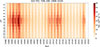 |
Figure 1. TEC variations from 1998 to 2024 for high latitudes, near Tromsø/Norway (70° N 20° E). |
2.2 Solar wind data
We decided to conduct our first analysis using solar wind data from the OMNI hourly “Near-Earth” magnetic field and plasma parameters, derived from several spacecraft at the L1 Lagrangian point and available for long time periods. OMNI 2 data (1-hour) is an hourly averaged multispacecraft combined parameters data that is time-shifted to the nose of the Earth’s bowshock. Solar wind magnetic field data with 1-hour resolution include parameters of the magnetic field: magnitude (B mag in nT), the x component of the magnetic field vector (B x in nT), the y component of the magnetic field vector (B y in nT), and the z component of the magnetic field vector (B z in nT) in the Geocentric Solar Magnetospheric (GSM) coordinate system. Also, low-resolution OMNI (LRO) solar wind plasma data with 1-hour resolution contain the proton density (n p in cm−3) and proton speed (v p in km/s). The outliers in the dataset, which are about 0.11% of the dataset, are removed and replaced with the basic linear interpolation method. For analyses using 1-minute-resolution EISCAT data, we use OMNI 1-minute “Near-Earth” data with the same parameters to obtain more accurate estimates of the time lag.
Derived solar wind parameters, such as the merging electric field (Kan & Lee 1979), are of great importance to represent the solar wind energy flux entering the magnetosphere through coupling. Kan & Lee (1979) merging electric field (E
m
= v
p
B
t
sin2(0.5θ)), has been proven to be well applicable for the correlation analysis with ionospheric parameters (e.g. Borries et al. 2024). E
m
(mV/m) is calculated using solar wind proton speed (v
p
), the magnitude of interplanetary magnetic field (IMF) in the yz plane (B
t
), and the theta angle (θ) between the z direction and the projection of IMF in the yz plane. The transversal magnetic field is  in nT and the clock angle is θ = arctan(B
y
/B
z
). The time series of the E
m
dataset is presented in Figure 2. The figure shows that 99.9% of the merging electric field Em ranges between 0 and 10 mV/m (grey solid line), and during individual events, it can exceed 40 mV/m. During solar minimum years, a decrease in the Em is visible from the annual moving average values between 0.5 and 1.5 mV/m (black solid line).
in nT and the clock angle is θ = arctan(B
y
/B
z
). The time series of the E
m
dataset is presented in Figure 2. The figure shows that 99.9% of the merging electric field Em ranges between 0 and 10 mV/m (grey solid line), and during individual events, it can exceed 40 mV/m. During solar minimum years, a decrease in the Em is visible from the annual moving average values between 0.5 and 1.5 mV/m (black solid line).
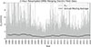 |
Figure 2. E m (mV/m) variation from 1998 to 2024, calculated from 1-hour OMNI near-Earth plasma and magnetic field data. The solid black line indicated the annual moving average of E m . |
2.3 Correlation with an offset applied to E m
The TEC and E m datasets from 1998 to 2024 are separated into 12 UT groups. We compute a Pearson correlation between TEC and E m over 90 winter days from 15 November to 15 February, centering on 1 January for each UT group. We apply an offset of hours, ranging from 0 to 48, to the 1-hour LRO OMNI solar wind dataset. We merge the 1-hour solar wind merging electric field that is floored to 2-hour resolution (without any averaging) with the 2-hour IGS TEC dataset to produce a matrix of correlation coefficients as a result for each winter. An example is shown for 1 January 2013 ±45 days in Figure 3, where each grid represents the correlation value for a unique UT and the corresponding offset hour. This method provides insight into the ionospheric delay, where we observe the highest correlation. Figure 3 shows high positive correlation values up to 0.8 with ≈2–5 h ionospheric delay time during the selected winter period. The positive correlation values remain high at 0.8, especially during the period from 18 UT to 06 UT (nighttime). As the IGS TEC dataset has a temporal resolution of 2 h, the inferred delay should be interpreted as an approximate response time. The diagonal stripes are observed to occur after every 24 h because the neighboring TEC values are related to each other. The same procedure is applied for each winter, from 1998 to 2024.
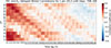 |
Figure 3. Delay in TEC and E m correlations during 1 January 2013 (DOY 1)±45, near Tromsø/Norway (70° N 20° E). The x-axis shows the time lag from 0 to 48 h, and the y-axis shows the UT. |
2.4 EISCAT Tromsø UHF radar measurements
The EISCAT UHF incoherent scatter radar at Tromsø Norway (geographic latitude: 69.58° N and longitude: 19.23° E) measures the key parameters in the ionosphere, including the electron density, electron and ion temperatures, and line-of-sight ion velocity. Those parameters can be used to estimate the electric field, conductivity, and currents. The Common Programme (CP) consists of pre-defined scan patterns of the EISCAT UHF antenna. CP2 scans in three or four high-elevation beams. In most cases, a CP2 scan includes one field-aligned beam and one vertical beam. The output data has a 1-minute resolution, covering all measured ranges from all beams.
We identified four CP2 campaigns of EISCAT Tromsø UHF radar applicable for the investigation and quantification of the ionospheric lag observed during winter nighttime. The selection criteria for these campaigns are based on the maximum data availability during winter nighttime, with multiple days without data gaps, and the availability of a field-aligned measurement. Each campaign consists of at least 3 consecutive nighttime measurements. Table 1 shows the selected dates of campaigns. In the next sections, the campaigns will be referred to with the corresponding campaign numbers written in the table.
The four EISCAT Tromsø UHF radar campaigns and their experiment types.
The EISCAT measurements analyzed by the Grand Unified Incoherent Scatter Design and Analysis Package (GUISDAP, Lehtinen & Huuskonen 1996) provide altitude profiles of electron density (N e ), ion and electron temperatures (T i and T e ), and the line-of-sight velocity. The data points were removed if the GUISDAP fit status ≠ 0, if the relative error of N e > 0.5, if the chi-square of the fit > 10, if the ion temperature < 50 K, if the N e > 1012 m−3 below 95 km altitude, if Te/Ti > 5, and if the errors of Te and Ti are > 1000 K.
Figure 4 shows the 1-minute resolution electron density (N e ) and electron temperature (T e ) measurements from all four beams between 90–500 km ionosphere, respectively, on the top and bottom panels for 2–6 February 2019, as one of the four selected EISCAT campaigns. This campaign is a CP-2 scanning experiment, where the radar dwells in four directions defined by azimuth and elevation pairs: (188°, 78°), (227°, 90°), (259°, 75°), (217°, 90°). From the top panel, it can be seen that in the ≈90–390 km range in the ionosphere during nighttime (18–6 UT), there is an increase with N e values exceeding 1011 m−3 especially in the E-region (90–150 km). This is typically produced by auroral particle precipitation during nighttime. During most of the nights in our campaign dates, we observe this E-region auroral precipitation, indicating that Tromsø is within the auroral oval range during the experiment interval (E-region auroral precipitation observed by nights: 2/3 Campaign 1, 5/5 Campaign 2, 8/10 Campaign 3, 4/4 Campaign 4). Also, according to a recent study investigating the location of EISCAT Tromsø within the auroral oval for a 20-year period, the radar is mostly within the oval in the evening for a broad range of geomagnetic activity index Hpo (see Fig. 2 in Enengl et al. 2023). This figure also shows the daily maxima in F-region N e due to solar EUV radiation. However, in this paper, we will focus only on nighttime variation.
The N e profiles are used to estimate the TEC (so-called EISCAT TEC) by integrating N e along altitude. Because GUISDAP fits N e at unevenly distributed height gates (between approximately 70–680 km range span), the original N e profiles are interpolated linearly with a height resolution of 1 km before the integration is applied. To estimate the 1-min resolution TEC, we separate the EISCAT N e into three regions of the ionosphere: E-region (90–150 km), F-region (150–500 km), and both regions combined (90–500 km) with 1 km vertical resolution. As a numerical integration method, we use the trapezoidal rule to approximate the TEC value from the area under the N e curve. To reject outlier TEC values, we use an exponentially weighted moving average. Data points are removed if the TEC value at a step deviates more than 10 standard deviations from the corresponding mean value, and missing values are linearly interpolated. A centered moving average over a 60-minute window is applied to the data to provide a smoother comparison of TEC across different ionospheric regions. For further investigation of the delay, we analyze the variation in EISCAT TEC with OMNI-merged electric field (E m ) at 1-minute resolution and present the results. The interval from 6 UT to 18 UT (daytime) is masked.
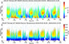 |
Figure 4. EISCAT Tromsø UHF radar 1-min electron density N e (top) and electron temperature T e (bottom) in the time period of 2–6 February 2019. |
To quantify the optimal lag with the highest correlation between EISCAT TEC and OMNI E m , we apply the method presented in Section 2.3 with an offset of about 0–4 h, varying in 0.25-hour (15-minute) steps. After applying the lag, we resample the 60-min moving-average data to 1-hour resolution and calculate the correlation value for each lag step only for data within the 18 UT to 6 UT (nighttime) interval.
2.5 AISstorm v2.1 ion pair production
AISstorm is a high-resolution numerical model that simulates atmospheric ionization rates caused by precipitating particles. It builds upon its predecessor, Atmospheric Ionization Model Osnabrück (AIMOS, Wissing & Kallenrode 2009) by separately addressing substorm periods. The model calculates 3D ionization rates from precipitating protons, electrons, and alpha particles with a temporal resolution of 30 min. AISstorm includes a sorting algorithm that assigns observations from polar-orbiting POES and Metop satellites to horizontal precipitation cells, utilizing data from the TED and MEPED detectors. Additionally, it incorporates data from the SEM detectors on GOES satellites to measure high-energy protons and alpha particles in the polar cap. The energy ranges for the model are 154 eV–500 MeV for protons, 154 eV–300 keV for electrons, and 4 MeV–500 MeV for alpha particles.
Mean flux maps were generated from 18 years of satellite data (2001–2018), categorized by Kp level, geomagnetic APEX (Richmond 1995), and magnetic local time (MLT) location, with a spatial resolution of up to 1° latitude and 3.75° longitude. These maps also account for substorm activity. Each flux map represents the typical spatial distribution of particle precipitation for a specific particle type on a global scale. Typical average flow maps from AIMOS are shown in Yakovchuk & Wissing (2019). The effective particle flux for each 30-minute interval is derived by scaling the precipitation maps using real-time measurements. By focusing on areas with high flux values, such as the auroral oval, this method minimizes the impact of noise in the data. The polar cap, however, is treated differently: the flux is directly obtained from satellite measurements, as long as the satellites are within a homogeneous flux area whose size varies with particle species and geomagnetic activity, as described in Yakovchuk & Wissing (2023).
The ionization profiles for each particle spectral interval are computed using the Monte Carlo method (Schröter et al. 2006), with atmospheric parameters taken from the HAMMONIA (Schmidt et al. 2006) and NRLMSISE-00 (Picone et al. 2002) models.
2.6 Geomagnetic activity index
In this study, the Auroral Electrojet (AE) index is used as a proxy for substorm activity to investigate the delay and origin of the ionospheric responses during winter nighttime. For the analyses using 1-minute-resolution EISCAT data, we use the OMNI 1-minute AE index. The AE index is defined by the difference between the upper and lower envelopes (AE = AU − AL) of the superposed H components of geomagnetic observatories in the auroral latitudes (Davis & Sugiura 1966). The threshold for the ionospheric activity to indicate typical substorms ranges from 250 nT to 600 nT (Pulkkinen et al. 2010). For multiple nights during the measured period, substorm activity is clearly identified by enhancements in the AE index, with values exceeding 250 nT.
3 Results
3.1 Solar wind forcing at Tromsø location and response time
The variations in TEC and Em correlations in winter are investigated by the correlation method, as explained in Section 2.3. For a more general representation, we average all winter (January 1 ±45 days) correlations over 26 years from 1998 to 2024 at the gridpoint of 70° N 20° E, close to Tromsø. Figure 5 shows the actual delay between the Em variability and the TEC response by using the average correlation coefficient for each UT and shift time of the Em. The delay is shown from 0 to 48 h during the 90-day period around January 1 (DOY 1) averaged from cross-correlated 26-year data in the corresponding UT group between 1998 and 2024. Each correlation grid value in the figure, corresponding to a specific time lag and UT, is calculated from 90 data points per year and later averaged over 26 years (≈2340 data points per grid). The color bar represents the correlation coefficient. Positive averaged correlation values of up to ≈0.4 are observed for all the UTs in winter, with local time-dependent variations. Especially between 18 UT and 6 UT, the average correlation value is observed to be higher. The correlation coefficient increases with an applied time lag and maximizes at about a value of ≈0.4 when there is an ≈2 h offset applied to Em. The reason that the maximum correlation is peaking about ≈0.4 value is that correlation values are affected by 26-year averaging, slight interpolation of the missing data, and the time lag applied to a 1-hour resolution Em data that is merged with a 2-hour dataset. And after ≈5 h offset, the correlation coefficient decreases. This result is observed for all hours between 18 UT and 6 UT.
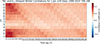 |
Figure 5. Delayed correlations of TEC and Em from 1998 to 2024, averaged from the correlations of each year’s winter period (January 1 ±45 days), near Tromsø/Norway (70° N 20° E). The x-axis shows the time lag from 0 to 48 h, and the y-axis shows the UT. |
Analyzing each grid point of the IGS TEC maps allows us to characterize the spatial properties of the positive winter nighttime correlation. Figure 6 shows a map of the correlation for a random example period of 90 days, centered on the 1st of January 2013 at 0 UT. The map shows the maximum correlation coefficients estimated for different delay times. The right panel shows the corresponding delay time where the correlation maximizes. It is clearly visible that the correlation coefficients maximize at the nightside, equatorward of the green oval, which is the 70° magnetic latitude circle indicating the approximate position of the auroral oval. The right panel shows a delay time of 1–3 h in the regions with the highest correlation coefficients. In the supplementary movie (Movie M1), it becomes visible that the region with the highest correlation moves around the 70° magnetic latitude circle with increasing UT time.
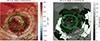 |
Figure 6. Correlation between IGS TEC and E m at 0 UT at each grid point of the IGS TEC maps in the time period of 01.01.2013 ±45 days, computed for a shifted solar wind by lag hours ranging from 0 to 48 h. Left: maximum correlation coefficient from the different lag hours (the gray shade indicates night condition). Right: lag hours at which the maximum correlation occurs (contour lines present the maximum correlation shown in the right panel). The green circles mark magnetic latitudes, where a bold circle of 70° N approximates Tromsø latitude. |
Since the results in Figure 6 indicate a relationship between the correlation pattern and magnetic latitude and local time, we convert the geographic coordinates of the correlation results into magnetic quasi-dipole latitude and magnetic local time (MLT). Figure 7 shows the correlation coefficients for each magnetic latitude and magnetic local time, averaged for the different UT times. The left panel shows that the main magnetic latitude of the high correlation is between 60 and 65° N, and the period of high correlation starts at about 21 MLT and remains strong until 6 MLT. The right panel shows that the corresponding time lag for the high correlation observed between 60 and 65° N is ≈2 h. Polewards of 65° N, the correlation decreases at most MLT times, except around midnight, when there is a clear period of increased correlation.
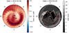 |
Figure 7. Correlation between IGS TEC and E m at each grid point of the IGS TEC maps in the time period of 01.01.2013 ±45 days, computed for a shifted solar wind by lag hours ranging from 0 to 48 h. The results are converted into geomagnetic coordinates (quasi dipole latitude in circles and magnetic local time in radial lines) and averaged over all UTs. Left: maximum correlation coefficient from the different lag hours. Right: lag hours at which the maximum correlation occurs (contour lines present the maximum correlation shown in the left panel). |
Figure 8 shows the 60-min centered moving average EISCAT TEC values for the different regions of the ionosphere. The bottom panel of Figure 8 shows the 1-minute resolution AE index during 2–6 February 2019, as one of the four selected EISCAT campaigns. The TEC values are observed to be lower compared to the IGS TEC values represented in Section 2.1 because the height limits of the measurement are lower for the EISCAT instrument. The plot shows that the TEC values in the E-region ionosphere are higher during nighttime than during the daytime. It was also observed that TEC values on some nights were as high as during daytime hours for the 90–500 km range (e.g., 1800-0600 UT on 02 Feb 2019.).
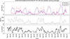 |
Figure 8. 60-min moving averages of EISCAT Tromsø UHF radar of Total Electron Content TEC (top panel), OMNI Auroral Electrojet (AE) index (bottom panel) and OMNI merging electric field (bottom panel) in the time period of 2–6 February 2019. The solid light pink dash-dotted line in the top panel corresponds to the 90–500 km TEC, the dotted dark blue line corresponds to the 150–500 km TEC, and the violet dashed line corresponds to the 90–150 km TEC. |
The top panel of Figure 9 shows an example of the variation of centered 60-minute moving averaged TEC measurements between 90–150 km (E-region), 150–500 km (F-region), and 90–500 km (E and F regions combined) ionosphere for the campaign #2 (2–6 February 2019). The bottom panel shows the scatter plots, respectively, for the E, F, and combined regions of the ionosphere. As clearly seen in the plot, the EISCAT TEC is correlated with the variation in OMNI Em, increasing with Em between 18 and 6 UT, with some lag. On the bottom panel of Figure 9, the scatter plot of 60-min moving averaged EISCAT TEC with OMNI Em is shown for the interval from 18 UT to 6 UT (nighttime). The data is resampled to 1-hour resolution to create the scatter plots, with no time lag applied. The correlation values for EISCAT TEC are found rE − region = 0.64, rF − region = 0.54, rCombined = 0.62. This shows that the ionospheric TEC for all regions is moderately correlated with OMNI Em.
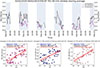 |
Figure 9. Top: EISCAT Tromsø UHF radar Total Electron Content TEC and OMNI merging electric field centered 60-min moving averages in the time period of 2–6 February 2019 from 18 UT to 6 UT. The dash-dotted light pink line corresponds to the 90–500 km TEC, the dotted dark blue line corresponds to the 150–500 km TEC, and the violet dashed line corresponds to the 90–150 km TEC. The black solid line represents OMNI E m . Bottom: Scatter plot of 60-min moving averages, and 1-hour resampled E m and TEC, respectively, for E, F, combined regions of the ionosphere from 18 UT to 6 UT. The confidence interval of 0.95 is shown by the red shaded area surrounding the red line. |
In Figure 10, the Pearson correlation values of height-integrated EISCAT TEC in three regions of the ionosphere and OMNI Em with an applied lag between 0–4 h are shown for the 2–6 February 2019 EISCAT campaign. Using this analysis, it is possible to identify the delay at which the correlation maximizes and the maximum Pearson correlation coefficient for each ionosphere altitude region. The E-region ionosphere (90–150 km) reaches the maximum correlation of rmax = 0.76 when the lag is t = 75 min. This lag time is small compared to the F-region ionosphere (150–500 km), with a lag time of t = 90 min, corresponding to rmax = 0.62. The combined region of the ionosphere (90–500 km) results in a maximum correlation value of rmax = 0.73 when t = 75 min. It should be noted that the large confidence intervals for the correlation coefficients (shaded regions) are due to the limited running time of the EISCAT UHF radar experiments.
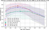 |
Figure 10. Lagged Pearson correlation values of 1-hour resampled EISCAT TEC and OMNI merging electric field E m between the time range of 18 and 6 UT on 2–6 February 2019. Pink color represents the E-region of the ionosphere (90–150 km), while green color is used to represent the F-region in the ionosphere (150–500 km) and lilac color for the combined region (90–500 km). The shaded area corresponds to the 0.95 confidence level of the correlation coefficient. |
This analysis with varying lag time is performed on the four other selected EISCAT campaigns during wintertime, and similar results are observed. There is an observed lag time in the response of the ionosphere to the solar wind for all campaigns as shown in Table 2 (and in Fig. A.3). We observe the shortest delays (45–90 min) of the maximum correlation value between the height-integrated EISCAT TEC and OMNI bow-shock shifted Em for three out of four events in the E-region (90–150 km). One can see that the lag times with the maximum correlation values for three out of four events are shorter, and the correlation values are higher in the E-region than in the F-region. The only exception is Campaign #1, where the lag is equal in all regions. The longest lag time of 135 min is found in the F-region. Another important outcome is that, across all campaigns, the maximum correlation is observed at a lag greater than zero. Averaged from all the campaigns, the lag is ≈71 min for E-region (90–150 km), ≈101 min for F-region (150–500 km), and ≈97 min for the combined regions (90–500 km).
The maximum Pearson correlation values of 1-hour resampled height-integrated EISCAT TEC in three regions of the ionosphere and OMNI E m with the corresponding lag time during 4 selected EISCAT Tromsø UHF campaigns.
Table 3 represents the ionospheric response to substorm activity, showing the maximum correlations for the corresponding time lag between EISCAT TEC and OMNI AE for all the campaigns (and Fig. A.4). Across all campaigns, the time lag is shorter in the E-region, ranging from 0 to 45 min. Higher correlation values are also observed in the E-region for three out of four campaigns. Averaged from all the campaigns, the lag is ≈18 min for E-region (90–150 km), ≈52 min for F-region (150–500 km), and ≈26 min for the combined regions (90–500 km).
The maximum Pearson correlation values of 1-hour resampled height-integrated EISCAT TEC in three regions of the ionosphere and OMNI AE index with the corresponding lag time during 4 selected EISCAT Tromsø UHF campaigns.
3.2 Ion pair production
In this study, we use AISstorm to provide a climatological view of electron precipitation patterns in the E and F regions of the ionosphere under similar conditions. To illustrate the average particle forcing in terms of the ion pair production (IPP) rates, we use the averages from the AISstorm model for the same winter period (2013-01-01 ±45 days) as in Figures 6 and 7.
Figure 11 shows the result. The left panel of Figure 11 illustrates the IPP rate due to precipitating electrons at approximately 111 km (E-layer), which corresponds to the peak auroral electron ionization rate in AISstorm. The IPP rate typically reaches its maximum during the early morning hours, between 1–3 MLT and around 65–70° APEX latitudes, but also shows significant contributions during the night and morning hours (8–18 MLT).
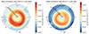 |
Figure 11. AISstorm ion pair production rate mean of precipitating electrons for the period ±45 days around 2013-01-01 on two altitude levels: left panel approx. 111 km and right panel approx. 259 km. |
The right panel of Figure 11 displays the IPP rate at 259 km, representing the F-layer. The IPP rate typically reaches its extended maximum values during the pre-midnight and midnight hours, between 21–3 MLT and around 70–80° APEX latitudes.
4 Discussion
4.1 E-region ionospheric response to solar wind variation
The spatial extent of the E-region particle precipitation, shown in Figure 11, largely coincides with the spatial extent of the high correlation of IGS TEC with solar wind merging electric field, shown in Figure 7. This is a strong indication that the auroral precipitation is a relevant process contributing to the ionospheric response to solar wind variability. The left panel of Figure 11 corresponds to the auroral electron precipitation with energies of > keV, where the ionization rate is high at nighttime. The latitudinal position of the IPP rate maximum is at about 66° APEX latitude. A comparison with long-term particle flux measurements that have been processed in the same manner as in Yakovchuk & Wissing (2019) (Figs. 3 and 4) but separated into different Kp-levels, indicating that we observe particle precipitation as it is typical for a relatively quiet geomagnetic period.
The peak values of the electron density reaching up to > 1012 m−3 in the lower E-region (mostly between 90 and 130 km) in campaign #2 can be attributed to auroral particle precipitation, as it is typically the only E-region ionization source during nighttime. This N e enhancement occurs simultaneously with the increase of electron temperature of about > 2000 K in the F-region (bottom panel of Fig. 4). The investigation of the four different EISCAT campaigns (cf. Fig. A.1) shows that the electron density increase observed in the E-region peaks around ≈110 km (from 22 UT to 03 UT). This agrees with the typical height of electron precipitation with a characteristic energy of a few keV, as described, e.g., in a statistical substorm study using the EISCAT UHF radar by Oyama et al. (2014).
Auroral particle precipitation affecting the E-region is a key component of substorm activity. Accordingly, our results show that there is a short time lag (≈18 min) between substorm activity and the E-region EISCAT TEC, as indicated by the correlation with the AE index, which serves as a proxy for substorm activity. Therefore, the estimated lag in the correlations between E m and E-region EISCAT TEC of ≈71 min (cf. Table 2) can be attributed to a large extent to the time period from the arrival of the solar wind until it results in substorm activity and auroral particle precipitation with a few keV (magnetospheric reconnection and substorm onset) in the E-region. This is confirmed by a study by Pulkkinen et al. (2010), who showed that the AE index is delayed by 40 min relative to the increased solar wind energy input. This is in good agreement, but slightly less than the 45–90 min delay estimated by using E-region EISCAT TEC and E m presented in Table 2. It should be noted that Pulkkinen et al. (2010) did not use OMNI solar wind data but instead applied a simple statistical method to estimate the time shift between the L1 point and the Earth’s bow shock, which may lead to differences in the magnetospheric response time compared to our results.
The increase of EISCAT TEC with OMNI E m in the E region with a 75-minute delay (cf. Fig. 10) can be explained by the time needed for the magnetospheric processes. This time period starts with the solar wind arrival at the bow shock to the subsolar magnetopause, continues with the energy storage in the magnetotail until the nightside reconnection and precipitation of energetic electrons from the plasma sheet begins.
Also Bargatze et al. (1985) reported that the typical substorm growth (magnetotail loading-unloading) duration is 60 min, supporting our interpretation that the E-region ionospheric response is primarily driven by auroral particle precipitation following energy accumulation in the magnetotail.
4.2 F-region ionospheric response to solar wind variation
The spatial preference of particle precipitation is very similar in the E- and F-region. Thus, soft-particle precipitation affecting the F-region electron density is also a candidate for increasing TEC with solar wind energy input (as shown in Fig. 11). The intensity of precipitating electrons is lower compared to E-region precipitation, as illustrated by a less strong peak of ion pair production in the F-region, compared to the E-region (cf. Fig. 11). Still, the peak of the correlation between IGS TEC and E m around 1–2 MLT, shown in the left panel of Figure 7, matches well with the right panel of Figure 11.
In our results from EISCAT campaigns (Table 2), the longest delays in the ionospheric response are observed in the F-region (150–500 km), with delays of 90–135 min. This is longer than what is observed in the E-region. Previously, we attributed the 45–90 min time lag to magnetospheric processes from the arrival of the solar wind until the onset of the substorm. However, the lag time of IGS TEC to Em being about ≈2 h and the lag time of EISCAT F-region TEC to E m being ≈90–135 min is much longer than the typical response time of particle precipitation, which has been estimated in the previous section. Blobs in the nightside associated with polar cap patches are found to produce more significant scintillation than blobs linked to auroral precipitation in the F-region, concluding that the nightside soft particle precipitation is unlikely to be the primary driver of F-region large-scale plasma structures (Jin et al. 2016). Considering the results of Jin et al. (2016); Enengl et al. (2023), F-region soft particle precipitation associated with substorm activity is not likely to be the primary cause of the large-scale F-region plasma structures on the nightside ionosphere, and therefore not the primary cause of the longer delay observed in this region.
Also, an indication for plasma convection processes across the polar cap can be found in Figure 7. There are high correlation values in the midnight sector (21-01 MLT) at latitudes 70°–90°, which cannot result from particle precipitation. The time lag between the maximum correlation between the merging electric field and TEC is observed to be about ≈2 h. We interpret this as the result of dayside-to-nightside polar cap plasma transport (convection). In addition, Borries et al. (2024) showed that there is a positive correlation between hmF2 and E m during winter daytime conditions at Tromsø and explained that this can result from plasma convection across the polar cap, which has an upward component at the dayside. The 2-hour time lag is of the same order as that found by Pedersen et al. (2023) for the correlation between the solar wind Newell coupling function and ionospheric field-aligned currents. The best correlation during storms, on average, was found with a 90-minute integration time for the Newell coupling function, but the optimal integration time varied between 80 and 140 min depending on the solar wind driver type.
Using the electron density measured by Swarm satellites between December 2013 and January 2014, Park et al. (2015) estimated the plasma convection along-track velocity component in the polar cap and found positive velocities (plasma drift in the flight direction of the Swarm satellites) mostly below 500 m/s from noon to midnight in the Northern Hemisphere (over 75° MLAT). There is uncertainty in estimating the transportation time and speed of patches/blobs within the polar cap. Larger velocities from Swarm estimates are compared with SuperDARN, yielding a correlation of ≈0.75 and a small bias of 50 m/s (Park et al. 2015). With the assumption that the plasma drift velocity in the F-region is on average 500 m/s ± 50 m/s, the polar cap latitude is 75° MLATs, and the straight path over the pole is 30° degrees of latitude (30 degrees × 111 km ≈ 3330 km distance from noon to midnight polar cap), the simple calculation leads us to the approximation that the time needed for a plasma to travel from the dayside to the nightside polar cap in a straight path is 111.1 ± 11.1 min ≈ 2 h. Using SuperDARN data, Eriksen et al. (2023) reported polar cap patch travel times of 92–104 min, which is close to our observed average F-region EISCAT TEC delay of ≈101 min across all campaigns. Since the approximate convection duration of 2 h during geomagnetic quiet conditions is in good agreement with the time delay in the F-region EISCAT TEC and IGS TEC reported here, it can be argued that the overall TEC response to solar wind variability mainly results from plasma convection.
The UHF observations of blobs indicate that plasma convection is another important process driving the ionosphere’s response to solar wind variations, with merged effects with particle precipitation. With a careful look at Campaign #2, Figure A.1, one can see a secondary electron density increase with a weaker peak at ≈250 km around 20–21 UT (hour 116–117). This is typical for the soft-particle precipitation with energies of a few hundred eV in the F-region (peaking around 250 km) and sometimes can merge with the effects from transported plasma patches/blobs (higher than 2050 km, Oyama et al. 2014; Cai et al. 2024). An example of the F-region electron density increasing due to soft particle precipitation observed by the EISCAT radar is given in Oyama et al. (2014), who explained that soft particle precipitation is sometimes accompanied by a long-lived plasma that drifts horizontally from the dayside (plasma patches).
Polar cap patches (PCPs) are high-density plasma structures in the F-region, which are transported from the dayside to the nightside via the ionospheric convection (Crowley 1996; Weber et al. 1984). When PCPs enter the nightside auroral oval via magnetotail reconnection, they are termed plasma blobs (Crowley et al. 2000). The blobs are further transported with the return flows in the oval. The arrival of the blobs at Tromsø can be detected by the UHF radar (e.g., Cai et al. 2024), which can be used to indicate the ionospheric convection process. The PCPs/blobs are usually identified by high-density plasma with relatively low electron temperature, compared to the background. In this study, the blobs can be clearly identified from the measurements in campaign #1. As shown in Figure A.2 in the appendix, a substorm took place between 21:30 and 01:30 UT (69.5–74.5) on 12 December 2013, which caused both E and F-region electron density enhancements due to auroral precipitations. Following that, a plasma blob is detected by the radar between 01:30 UT and 07:30 UT (74.5–79.5) on 12 December 2013, characterized by increased F-region electron density above 250 km altitude and decreased electron temperature. Compared with campaign #1, the indication of plasma blobs during campaign #2 (Fig. 4) is not as clear, because the electron density was lower above 250 km than below with relatively high T e . Similarly, blobs are observed also in campaigns #3 and #4 (figures not shown). We observe increased electron density in the F-region on all nights during our four EISCAT campaigns.
During one of our EISCAT campaigns (campaign #1), we showed equal lag time in the TEC and E m correlations in the E and the F-region ionosphere with 90 min. In campaign #1, during the night of 9 January and 11 January 2013, the electron density is strongly enhanced as the F-region soft-particle precipitation is accompanied by dense plasma blobs. The F-region ionospheric response in this case (90 min) is observed to be shorter than in the other campaigns (≈101 min). This short F-region response time can result from two processes: either soft-particle precipitation in the F-region or polar cap patches/blobs sitting in the middle of the convection flow channel, where the convection speed is higher than the average (Oksavik et al. 2010). F-region soft particle precipitation can be excluded as a source mechanism because during the second night, the auroral precipitation signatures are not clear in the EISCAT data, as E-region electron density and F-region ion temperature are not enhanced, and AE < 75 nT does not indicate substorm activity. However, during all the nights between 9 and 12 January 2013, dense blobs were observed. Hence, this campaign supports the argument that the electron density enhancement in the F-region depends predominantly on convection.
5 Summary and conclusions
This paper highlights the processes driving the high-latitude ionospheric response to the solar wind forcing during winter nighttime conditions. By analyzing TEC estimates from different sources and OMNI E m data from 1998 to 2024 using a lagged correlation method, we investigate the temporal and spatial characteristics of the ionospheric response to solar wind variability to identify dominant mechanisms and responses in the E and F regions. The EISCAT observations were very helpful to differentiate the high-latitude winter nighttime ionospheric response driven by particle precipitation and plasma convection.
Our results show that:
-
There is a persistent ionospheric response to solar wind variability in the high-latitude ionosphere during winter nighttime. It is characterized by a positive correlation between IGS TEC and OMNI Em centered near the auroral oval at about 65°–70° magnetic latitude in the MLT sector 21-06. In the midnight sector (23-00 MLT), it reaches from 65° to the pole. The correlation is strongest at an approximate lag time of ≈2 h. This is supported by higher-resolution EISCAT TEC analysis (≈70–100 min).
-
Auroral particle precipitation driven by substorm activity causes a significant correlation of the EISCAT E-region TEC with Em. This E-region response is caused by precipitation effects during substorms, and the observed delay in the E-region TEC variability relative to Em of 45–90 min can be fully attributed to magnetospheric processes (loading and unloading).
-
The F-region TEC has been shown to be mainly driven by convection processes, which result in a time delay of approximately 2 h to the solar wind energy input. As observed in most campaigns, there is a merged effect from particle precipitation and convection processes in the F-region, with a delay of 90–135 min.
-
In individual cases, the F-region response in the EISCAT TEC and OMNI Em correlations could be as short as ≈90 min (e.g., Campaign #1). This is explained by the enhanced electron density resulting from denser polar cap patches/blobs convected into the radar volume.
In conclusion, both precipitation effects and plasma convection are strong drivers of the ionospheric variability at high latitudes. The auroral precipitation drives the E-region ionospheric response with an average delay of 45–90 min to the solar wind E m , and the plasma convection is a main source of the F-region response with an average delay of ≈100–120 min. The vertically integrated TEC provided by the IGS TEC maps reflects most of the time the F-region response. However, during substorm activity, the E-region response can temporarily be the dominant driver of IGS TEC variability. In the future, we also need to investigate if existing physics-based models can reproduce this ionospheric response and can help analyze the relevant processes.
Acknowledgments
We acknowledge NASA Goddard Space Flight Center for providing hourly “Near-Earth” solar wind magnetic field and plasma data via OMNIWEB, and the International GNSS Service (IGS) for providing TEC maps used here. EISCAT is an international association supported by research organizations in China (CRIRP), Finland (SA), Japan (NIPR and ISEE), Norway (NFR), Sweden (VR), and the United Kingdom (UKRI). The open source Python package GeospaceLAB (https://github.com/JouleCai/geospacelab) is used to search EISCAT campaigns and check the quicklook plots (Cai et al. 2022). We are also very grateful to F. Günzkofer, F. Heymann, T. Kodikara, and H. Sato for fruitful discussions. The editor thanks Onyinye Gift Nwankwo and an anonymous reviewer for their assistance in evaluating this paper.
Funding
This research has been supported by the DLR/DAAD Research Fellowships, Doctoral Studies in Germany (grant no. 57622551). Part of this work is carried out at the University of Oulu with support from the SCOSTEP SVS 2024 program. Claudia Borries and Jürgen Kusche acknowledge support by the German Research Foundation DFG in the framework of the Research Unit FOR 5405 (Magnetosphere, Ionosphere, Plasmasphere and Thermosphere as a coupled system). Anita Aikio acknowledges the support by Research Council of Finland, projects INTERSECT 348782 and SpaceResilience 374100.
Conflicts of interest
The authors declare no Conflict of Interest.
Data availability statement
EISCAT Tromsø UHF radar data are available at: https://madrigal.eiscat.se/madrigal/ (last access on 31 March 2026). Solar wind data and AE index are provided by OMNIWEB: https://spdf.gsfc.nasa.gov/pub/data/omni/ (last access on 31 March 2026). IGS TEC data are available at: https://cdaweb.gsfc.nasa.gov/pub/data/gps/ (last access on 31 March 2026).
Supplementary material
Movie M1: Correlation between IGS TEC and Em for all UTs in the time period of 01.01.2013 ±45 days, computed for a shifted solar wind by lag hours ranging from 0 to 48 h. Left: maximum correlation coefficient from the different lag hours (the gray shade indicates night condition). Right: lag hours at which the maximum correlation occurs (contour lines present the maximum correlation shown in the right panel). The green bold circle approximates magnetic Tromsø latitude. Access Supplementary Material
References
- Bargatze LF, Baker DN, McPherron RL, Hones EW. 1985. Magnetospheric impulse response for many levels of geomagnetic activity. J Geophys Res: Space Phys 90(A7): 6387–6394. https://doi.org/10.1029/JA090iA07p06387. [Google Scholar]
- Borries C, Iochem P, Tasnim S, Davis F. 2024. Persistent high-latitude ionospheric response to solar wind forcing. J Space Weather Space Clim 14: 33. https://doi.org/10.1051/swsc/2024029. [Google Scholar]
- Buchau J, Reinisch BW, Anderson DN, Weber EJ, Dozois C. 1988. Polar cap plasma convection measurements and their relevance to the modeling of the high-latitude ionosphere. Radio Sci 23(4): 521–536. https://doi.org/10.1029/rs023i004p00521. [Google Scholar]
- Cai L, Aikio A, Kullen A, Deng Y, Zhang Y, et al. 2022. GeospaceLAB: Python package for managing and visualizing data in space physics. Front Astron Space Sci 9: 1023163. https://doi.org/10.3389/fspas.2022.1023163. [Google Scholar]
- Cai L, Aikio A, Oyama S, Ivchenko N, Vanhamäki H, et al. 2024. Effect of polar cap patches on the high-latitude upper thermospheric winds. J Geophys Res: Space Phys 129(8): e2024JA032819. https://doi.org/10.1029/2024JA032819. [Google Scholar]
- Consolini G, Tozzi R, De Michelis P, Coco I, Giannattasio F, et al. 2021. High-latitude polar pattern of ionospheric electron density: Scaling features and IMF dependence. J Atmos Sol-Terr Phys 217: 105,531. https://doi.org/10.1016/j.jastp.2020.105531. [Google Scholar]
- Cowley SWH. 1984. Solar wind control of magnetospheric convection. In: Achievements of the International Magnetospheric Study (IMS). Proceedings of an International Symposium, Graz, Austria, 26-28 June 1984, Battrick B, Rolfe E, Roederer JG (Eds.), Vol. 217 of ESA Special Publication, pp. 483–494. [Google Scholar]
- Crowley G. 1996. Critical review of ionospheric patches and blobs. In: Review of Radio Science, Stone WR (Ed.), Vol. 619, Oxford University Press, Oxford, UK, pp. 619–648. ISBN 0-19-856532-1. [Google Scholar]
- Crowley G, Ridley AJ, Deist D, Wing S, Knipp DJ, et al. 2000. Transformation of high-latitude ionospheric F region patches into blobs during the March 21, 1990, storm. J Geophys Res: Space Phys 105(A3): 5215–5230. https://agupubs.onlinelibrary.wiley.com/doi/abs/10.1029/1999JA900357. [Google Scholar]
- Davis TN, Sugiura M. 1966. Auroral electrojet activity index AE and its universal time variations. J Geophys Res 71(3): 785–801. https://doi.org/10.1029/JZ071i003p00785. [CrossRef] [Google Scholar]
- Enengl F, Kotova D, Jin Y, Clausen LB, Miloch WJ. 2023. Ionospheric plasma structuring in relation to auroral particle precipitation. J Space Weather Space Clim 13: 1. https://doi.org/10.1051/swsc/2022038. [CrossRef] [EDP Sciences] [Google Scholar]
- Eriksen NK, Lorentzen DA, Oksavik K, Baddeley L, Hosokawa K, et al. 2023. On the creation, depletion, and end of life of polar cap patches. J Geophys Res: Space Phys 128(12): e2023JA031739. https://doi.org/10.1029/2023JA031739. [Google Scholar]
- Evans D, Jacobsen T, Maehlum B, Skovli G, Wedde T. 1972. Low energy electron precipitation and the ionospheric F-region in and north of the auroral zone. Planet Space Sci 20(2): 233–251. https://doi.org/10.1016/0032-0633(72)90105-5. [Google Scholar]
- Geethakumari GP, Aikio AT, Cai L, Vanhamäki H, Virtanen II, et al. 2024. Total electron content variations during an HSS/SIR-driven geomagnetic storm at high and mid latitudes. J Geophys Res: Space Phys 129(12): e2024JA033192. https://doi.org/10.1029/2024JA033192. [Google Scholar]
- Heelis R, Hanson W. 1980. High-latitude ion convection in the nighttime F region. J Geophys Res: Space Phys 85(A5): 1995–2002. https://doi.org/10.1029/ja085ia05p01995. [Google Scholar]
- Jin Y, Moen JI, Miloch WJ, Clausen LBN, Oksavik K. 2016. Statistical study of the GNSS phase scintillation associated with two types of auroral blobs. J Geophys Res: Space Phys 121(5): 4679–4697. https://doi.org/10.1002/2016JA022613. [Google Scholar]
- Kan JR, Lee LC. 1979. Energy coupling function and solar wind-magnetosphere dynamo. Geophys Res Lett 6(7): 577–580. https://doi.org/10.1029/gl006i007p00577. [Google Scholar]
- Labelle J, Sica RJ, Kletzing C, Earle GD, Kelley MC, et al. 1989. Ionization from soft electron precipitation in the auroral F region. J Geophys Res: Space Phys 94(A4): 3791–3798. https://doi.org/10.1029/JA094iA04p03791. [Google Scholar]
- Lehtinen MS, Huuskonen A. 1996. General incoherent scatter analysis and GUISDAP. J Atmos Terr Phys 58(1–4): 435–452. https://doi.org/10.1016/0021-9169(95)00047-x. [Google Scholar]
- Lilensten J, Pibaret B, Lemieux-Dudon B. 2016. A morphological study of the integrated total electron content and F region parameters using EISCAT in the frame of space weather, EISCAT Technical Report 04/54. URL https://eiscat.se/technology/wp-content/uploads/sites/2/2026/03/Technical-Note-2004_54.pdf. [Google Scholar]
- Lockwood M. 1991. The excitation of ionospheric convection. J Atmos Terr Phys 53(3–4): 177–199. https://doi.org/10.1016/0021-9169(91)90103-e. [Google Scholar]
- Lockwood M, Cowley SWH, Freeman MP. 1990. The excitation of plasma convection in the high-latitude ionosphere. J Geophys Res: Space Phys 95(A6): 7961–7972. https://doi.org/10.1029/ja095ia06p07961. [Google Scholar]
- Oksavik K, Barth VL, Moen J, Lester M. 2010. On the entry and transit of high-density plasma across the polar cap. J Geophys Res: Space Phys 115(A12). https://doi.org/10.1029/2010JA015817. [Google Scholar]
- Oyama S, Miyoshi Y, Shiokawa K, Kurihara J, Tsuda TT, et al. 2014. Height-dependent ionospheric variations in the vicinity of nightside poleward expanding aurora after substorm onset. J Geophys Res: Space Phys 119(5): 4146–4156. https://doi.org/10.1002/2013JA019704. [Google Scholar]
- Oyama S, Kero A, Rodger CJ, Clilverd MA, Miyoshi Y, et al. 2017. Energetic electron precipitation and auroral morphology at the substorm recovery phase. J Geophys Res: Space Phys 122(6): 6508–6527. https://doi.org/10.1002/2016ja023484. [Google Scholar]
- Park J, Lühr H, Stolle C, Malhotra G, Baker JBH, et al. 2015. Estimating along-track plasma drift speed from electron density measurements by the three Swarm satellites. Ann Geophys 33(7): 829–835. https://doi.org/10.5194/angeo-33-829-2015. [Google Scholar]
- Pedersen MN, Vanhamäki H, Aikio AT. 2023. Comparison of field-aligned current responses to HSS/SIR, sheath, and magnetic cloud driven geomagnetic storms. Geophys Res Lett 50(11): e2023GL103151. https://doi.org/10.1029/2023GL103151. [Google Scholar]
- Picone JM, Hedin AE, Drob DP, Aikin AC. 2002. NRLMSISE-00 empirical model of the atmosphere: Statistical comparisons and scientific issues. J Geophys Res: Space Phys 107(A12): SIA 15–1–SIA 15–16. URL https://agupubs.onlinelibrary.wiley.com/doi/abs/10.1029/2002JA009430. [Google Scholar]
- Prölss G, Roemer M, Slowey J. 1988. Dissipation of solar wind energy in the Earth’s upper atmosphere: The geomagnetic activity effect. Adv Space Res 8(5–6): 215–261. https://doi.org/10.1016/0273-1177(88)90043-9. [CrossRef] [Google Scholar]
- Pulkkinen TI, Palmroth M, Janhunen P, Koskinen HEJ, McComas DJ, et al. 2010. Timing of changes in the solar wind energy input in relation to ionospheric response. J Geophys Res: Space Phys 115(A5). https://doi.org/10.1029/2010JA015764. [Google Scholar]
- Richmond AD. 1995. Ionospheric electrodynamics using magnetic apex coordinates. J Geomagn Geoelectr 47(2): 191–212. https://doi.org/10.5636/jgg.47.191. [CrossRef] [Google Scholar]
- Rodger AS, Pinnock M, Dudeney JR, Baker KB, Greenwald RA. 1994. A new mechanism for polar patch formation. J Geophys Res: Space Phys 99(A4): 6425–6436. https://doi.org/10.1029/93JA01501. [Google Scholar]
- Schmidt H, Brasseur GP, Charron M, Manzini E, Giorgetta MA, et al. 2006. The HAMMONIA chemistry climate model: Sensitivity of the mesopause region to the 11-year solar cycle and CO2 doubling. J Clim 19(16): 3903–3931. URL https://journals.ametsoc.org/view/journals/clim/19/16/jcli3829.1.xml. [Google Scholar]
- Schröter J, Heber B, Steinhilber F, Kallenrode M. 2006. Energetic particles in the atmosphere: A Monte-Carlo simulation. Adv Space Res 37(8): 1597–1601. https://doi.org/10.1016/j.asr.2005.05.085, URL https://www.sciencedirect.com/science/article/pii/S0273117705007064. [Google Scholar]
- Schunk RW, Nagy AF. 2000. Ionospheres: Physics, Plasma Physics, and Chemistry, Cambridge University Press. ISBN 9780511551772. https://doi.org/10.1017/cbo9780511551772. [Google Scholar]
- Schunk R, Zhu L. 2008. Response of the ionosphere-thermosphere system to magnetospheric processes. J Atmos Sol-Terr Phys 70(18): 2358–2373. https://doi.org/10.1016/j.jastp.2008.07.003. [Google Scholar]
- Sojka JJ, Schunk RW. 1987. Theoretical study of the high-latitude ionosphere’s response to multicell convection patterns. J Geophys Res: Space Phys 92(A8): 8733–8744. https://doi.org/10.1029/ja092ia08p08733. [Google Scholar]
- Wakabayashi M, Ono T. 2006. Electron density measurement under the influence of auroral precipitation and electron beam injection during the DELTA campaign. Earth Planets Space 58(9): 1147–1154. https://doi.org/10.1186/BF03352004. [Google Scholar]
- Weber EJ, Buchau J, Moore JG, Sharber JR, Livingston RC, et al. 1984. F layer ionization patches in the polar cap. J Geophys Res: Space Phys 89(A3): 1683–1694. https://doi.org/10.1029/JA089iA03p01683. [Google Scholar]
- Weber EJ, Klobuchar JA, Buchau J, Carlson HC, Livingston RC, et al. 1986. Polar cap F layer patches: Structure and dynamics. J Geophys Res: Space Phys 91(A11): 12,121–12,129. https://doi.org/10.1029/JA091iA11p12121. [Google Scholar]
- Wissing JM, Kallenrode M-B. 2009. Atmospheric ionization module Osnabrück (AIMOS): A 3-D model to determine atmospheric ionization by energetic charged particles from different populations. J Geophys Res: Space Phys 114(A6). URL https://agupubs.onlinelibrary.wiley.com/doi/abs/10.1029/2008JA013884. [Google Scholar]
- Yakovchuk O, Wissing JM. 2019. Magnetic local time asymmetries in precipitating electron and proton populations with and without substorm activity. Ann Geophys 37(6): 1063–1077. URL https://angeo.copernicus.org/articles/37/1063/2019/. [CrossRef] [Google Scholar]
- Yakovchuk O, Wissing JM. 2023. Polar particle flux distribution and its spatial extent. J Space Weather Space Clim 13: 9. URL https://doi.org/10.1051/swsc/2023009. [Google Scholar]
Appendix A
Supporting figures
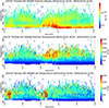 |
Figure A.1. The extended plot of EISCAT electron density (Ne), electron temperature (Te), and ion temperature (Ti), respectively, between 90 and 500 km for the campaign #2, from 18:00 to 23:00 UT on 6 February 2019. |
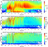 |
Figure A.2. The extended plot of EISCAT electron density (Ne), electron temperature (Te), and ion temperature (Ti), respectively, between 90 and 500 km for the campaign #1, from 11 January 2013 20:00 to 12 January 2013 08:00 UT. |
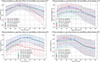 |
Figure A.3. Lagged Pearson correlation values of 1-hour resampled EISCAT TEC and OMNI merging electric field Em between the time range of 18 and 6 UT on 9–12 January 2013 (left top), 2–6 February 2019 (right top), 19–29 January 2010 (left bottom), and 6–9 February 2007 (right bottom). Pink represents the E-region of the ionosphere (90–150 km), green the F-region (150–500 km), and lilac the combined region (90–500 km). The shaded area corresponds to the 0.95 confidence level of the correlation coefficient. |
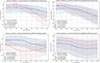 |
Figure A.4. Lagged Pearson correlation values of 1-hour resampled EISCAT TEC and OMNI Auroral Electrojet AE between the time range of 18 and 6 UT on 9–12 January 2013 (left top), 2–6 February 2019 (right top), 19–29 January 2010 (left bottom), and 6–9 February 2007 (right bottom). Pink represents the E-region of the ionosphere (90–150 km), green the F-region (150–500 km), and lilac the combined region (90–500 km). The shaded area corresponds to the 0.95 confidence level of the correlation coefficient. |
Cite this article as: Iochem P, Borries C, Tasnim S, Wissing JM, Kusche J, Aikio A, Cai L, Virtanen I & Ellahouny N. 2026. Sources of the high latitude ionosphere variability during winter nighttime. J. Space Weather Space Clim. 16, 23. https://doi.org/10.1051/swsc/2026018.
All Tables
The maximum Pearson correlation values of 1-hour resampled height-integrated EISCAT TEC in three regions of the ionosphere and OMNI E m with the corresponding lag time during 4 selected EISCAT Tromsø UHF campaigns.
The maximum Pearson correlation values of 1-hour resampled height-integrated EISCAT TEC in three regions of the ionosphere and OMNI AE index with the corresponding lag time during 4 selected EISCAT Tromsø UHF campaigns.
All Figures
|
Figure 1. TEC variations from 1998 to 2024 for high latitudes, near Tromsø/Norway (70° N 20° E). |
| In the text | |
|
Figure 2. E m (mV/m) variation from 1998 to 2024, calculated from 1-hour OMNI near-Earth plasma and magnetic field data. The solid black line indicated the annual moving average of E m . |
| In the text | |
|
Figure 3. Delay in TEC and E m correlations during 1 January 2013 (DOY 1)±45, near Tromsø/Norway (70° N 20° E). The x-axis shows the time lag from 0 to 48 h, and the y-axis shows the UT. |
| In the text | |
|
Figure 4. EISCAT Tromsø UHF radar 1-min electron density N e (top) and electron temperature T e (bottom) in the time period of 2–6 February 2019. |
| In the text | |
|
Figure 5. Delayed correlations of TEC and Em from 1998 to 2024, averaged from the correlations of each year’s winter period (January 1 ±45 days), near Tromsø/Norway (70° N 20° E). The x-axis shows the time lag from 0 to 48 h, and the y-axis shows the UT. |
| In the text | |
|
Figure 6. Correlation between IGS TEC and E m at 0 UT at each grid point of the IGS TEC maps in the time period of 01.01.2013 ±45 days, computed for a shifted solar wind by lag hours ranging from 0 to 48 h. Left: maximum correlation coefficient from the different lag hours (the gray shade indicates night condition). Right: lag hours at which the maximum correlation occurs (contour lines present the maximum correlation shown in the right panel). The green circles mark magnetic latitudes, where a bold circle of 70° N approximates Tromsø latitude. |
| In the text | |
|
Figure 7. Correlation between IGS TEC and E m at each grid point of the IGS TEC maps in the time period of 01.01.2013 ±45 days, computed for a shifted solar wind by lag hours ranging from 0 to 48 h. The results are converted into geomagnetic coordinates (quasi dipole latitude in circles and magnetic local time in radial lines) and averaged over all UTs. Left: maximum correlation coefficient from the different lag hours. Right: lag hours at which the maximum correlation occurs (contour lines present the maximum correlation shown in the left panel). |
| In the text | |
|
Figure 8. 60-min moving averages of EISCAT Tromsø UHF radar of Total Electron Content TEC (top panel), OMNI Auroral Electrojet (AE) index (bottom panel) and OMNI merging electric field (bottom panel) in the time period of 2–6 February 2019. The solid light pink dash-dotted line in the top panel corresponds to the 90–500 km TEC, the dotted dark blue line corresponds to the 150–500 km TEC, and the violet dashed line corresponds to the 90–150 km TEC. |
| In the text | |
|
Figure 9. Top: EISCAT Tromsø UHF radar Total Electron Content TEC and OMNI merging electric field centered 60-min moving averages in the time period of 2–6 February 2019 from 18 UT to 6 UT. The dash-dotted light pink line corresponds to the 90–500 km TEC, the dotted dark blue line corresponds to the 150–500 km TEC, and the violet dashed line corresponds to the 90–150 km TEC. The black solid line represents OMNI E m . Bottom: Scatter plot of 60-min moving averages, and 1-hour resampled E m and TEC, respectively, for E, F, combined regions of the ionosphere from 18 UT to 6 UT. The confidence interval of 0.95 is shown by the red shaded area surrounding the red line. |
| In the text | |
|
Figure 10. Lagged Pearson correlation values of 1-hour resampled EISCAT TEC and OMNI merging electric field E m between the time range of 18 and 6 UT on 2–6 February 2019. Pink color represents the E-region of the ionosphere (90–150 km), while green color is used to represent the F-region in the ionosphere (150–500 km) and lilac color for the combined region (90–500 km). The shaded area corresponds to the 0.95 confidence level of the correlation coefficient. |
| In the text | |
|
Figure 11. AISstorm ion pair production rate mean of precipitating electrons for the period ±45 days around 2013-01-01 on two altitude levels: left panel approx. 111 km and right panel approx. 259 km. |
| In the text | |
|
Figure A.1. The extended plot of EISCAT electron density (Ne), electron temperature (Te), and ion temperature (Ti), respectively, between 90 and 500 km for the campaign #2, from 18:00 to 23:00 UT on 6 February 2019. |
| In the text | |
|
Figure A.2. The extended plot of EISCAT electron density (Ne), electron temperature (Te), and ion temperature (Ti), respectively, between 90 and 500 km for the campaign #1, from 11 January 2013 20:00 to 12 January 2013 08:00 UT. |
| In the text | |
|
Figure A.3. Lagged Pearson correlation values of 1-hour resampled EISCAT TEC and OMNI merging electric field Em between the time range of 18 and 6 UT on 9–12 January 2013 (left top), 2–6 February 2019 (right top), 19–29 January 2010 (left bottom), and 6–9 February 2007 (right bottom). Pink represents the E-region of the ionosphere (90–150 km), green the F-region (150–500 km), and lilac the combined region (90–500 km). The shaded area corresponds to the 0.95 confidence level of the correlation coefficient. |
| In the text | |
|
Figure A.4. Lagged Pearson correlation values of 1-hour resampled EISCAT TEC and OMNI Auroral Electrojet AE between the time range of 18 and 6 UT on 9–12 January 2013 (left top), 2–6 February 2019 (right top), 19–29 January 2010 (left bottom), and 6–9 February 2007 (right bottom). Pink represents the E-region of the ionosphere (90–150 km), green the F-region (150–500 km), and lilac the combined region (90–500 km). The shaded area corresponds to the 0.95 confidence level of the correlation coefficient. |
| In the text | |
Current usage metrics show cumulative count of Article Views (full-text article views including HTML views, PDF and ePub downloads, according to the available data) and Abstracts Views on Vision4Press platform.
Data correspond to usage on the plateform after 2015. The current usage metrics is available 48-96 hours after online publication and is updated daily on week days.
Initial download of the metrics may take a while.