


| Issue |
J. Space Weather Space Clim.
Volume 16, 2026
|
|
|---|---|---|
| Article Number | 21 | |
| Number of page(s) | 12 | |
| DOI | https://doi.org/10.1051/swsc/2026016 | |
| Published online | 12 June 2026 | |
Technical Article
Bridging the measurement gap between MeV and GeV particles in space: Design and first results of the CHerenkov Atmospheric Observation System (CHAOS)
Christian-Albrechts-Universität zu Kiel, Leibnizstraße 11, Kiel D-24118 Schleswig-Holstein, Germany
* Corresponding author: This email address is being protected from spambots. You need JavaScript enabled to view it.
Received:
30
January
2026
Accepted:
17
April
2026
Abstract
Solar energetic particles are of major importance for understanding space weather. While numerous spaceborne instruments measure the particles with energies below several MeV and ground-based measurements address the particles with energies above approximately 1 GeV, the intermediate energies are sparsely covered. The CHerenkov Atmospheric Observation System (CHAOS) is a particle detector for solar energetic particles and galactic cosmic rays that bridges this gap in energy coverage. CHAOS uses multiple solid-state detectors and a bismuth germanium oxide scintillator to enable energy-resolved measurements of different particle species using the dE/dx − dE/dx method. Furthermore, an aerogel Cherenkov detector serves as a velocity threshold detector. The Cherenkov detector allows a clean measurement of protons with kinetic energies of tens of MeV up to 2.1 GeV, free from electron contamination. In this paper, we describe the design of CHAOS and show the first results to demonstrate the instrument’s capabilities. For this, we use measurements obtained during a stratospheric balloon flight as part of the BEXUS 35 campaign as well as measurements conducted at the CERN-EU high-energy Reference Field and compare them with GEANT4 Monte Carlo simulations.
Key words: Cherenkov effect / Aerogel / Solar energetic particles / Galactic cosmic rays / BEXUS / CERF
© A. Pohley et al., Published by EDP Sciences 2026
 This is an Open Access article distributed under the terms of the Creative Commons Attribution License (https://creativecommons.org/licenses/by/4.0), which permits unrestricted use, distribution, and reproduction in any medium, provided the original work is properly cited.
1 Introduction
The Solar System and the numerous spacecraft within it are constantly exposed to charged particle radiation made up of electrons, protons and heavier nuclei. Major components of this radiation are solar energetic particles (SEPs) (Reames 2023) and galactic cosmic rays (GCRs; Blasi 2013; Grenier et al. 2015). In this paper, the design and first results of the CHerenkov Atmospheric Observation System (CHAOS), a particle detector for solar energetic particles and galactic cosmic rays covering the energy range from tens of MeV to multiple GeV, are presented. CHAOS was developed as part of the Balloon EXperiments for University Students (BEXUS) 35 campaign, which took place in October 2024.
The main purpose of CHAOS is to serve as a prototype for a possible particle monitor onboard the European Space Agency (ESA)’s planned Advanced Telescope for High-ENergy Astrophysics (Athena; Nandra et al. 2013; Barret et al. 2020). Marelli et al. (2021) and Gastaldello et al. (2022) have shown that GCR particles contribute to the background measured by X-ray telescopes such as the Athena. Detailed knowledge of this particle-induced background is necessary to achieve the design goal of Athena, which is to measure X-ray fluxes with unprecedented precision. To characterize the particle fluxes, the Department for Extraterrestrial Physics at Kiel University proposed the Athena High-Energy Particle Monitor (AHEPaM), which builds on the compact design of the High Energy Telescope (HET; Rodríguez-Pacheco et al. 2020) onboard Solar Orbiter (SolO; Müller et al. 2020) with two additional aerogel Cherenkov detectors. The Cherenkov detectors serve as velocity threshold detectors and utilize the energy-dependent emission of photons in the aerogel due to the Cherenkov effect (Cherenkov 1934, 1937). A similar aerogel Cherenkov detector was already used for the Kiel Electron Telescope (KET; Kunow et al. 1991). The AHEPaM design bridges the gap in energy coverage between small instruments like the HET and considerably larger instruments such as the Payload for Antimatter Matter Exploration and Light-nuclei Astrophysics (PAMELA; Picozza et al. 2007) and the Alpha Magnetic Spectrometer (AMS-02; Aguilar et al. 2015). While doing this, AHEPaM maintains a compact and lightweight design, for which CHAOS is a first prototype. In addition to the measurement of GCRs, the covered energy range of tens of MeV to multiple GeV makes the design of the AHEPaM and CHAOS of special interest for the space weather community to monitor SEPs.
The paper is divided into six sections. Section 2 provides an overview of the experimental setup of CHAOS and the working principles of the individual detector stages. In Section 3, the three data sets used in this paper are described. One data set was acquired during the BEXUS 35 stratospheric balloon flight in northern Sweden in October 2024, while another is based on measurements performed at the CERN-EU high-energy Reference Field (CERF; Mitaroff & Silari 2002) in May 2025. These data sets are compared with detailed GEometry ANd Tracking (GEANT4; Agostinelli et al. 2003; Allison et al. 2006, 2016) Monte Carlo simulations of the instrument, which are the third data set. In Section 4, threshold values for the aerogel Cherenkov detector of CHAOS are defined. Section 5 shows how different particle species are discriminated by CHAOS and demonstrates how the contamination of proton measurements by high-energy electrons can be removed. Finally, the discussion and conclusions are presented in Section 6.
2 Instrument description
To perform measurements of individual charged particles, CHAOS uses a combination of five different detector stages, denoted A to E, which together make up the sensor head shown in Figure 1. The first stage is a solid state detector (SSD) and is denoted SSD Stage A. It is followed by Cherenkov Stage B. This stage consists of an aerogel block and a photomultiplier tube (PMT) to measure the Cherenkov photons produced within the aerogel. The third detector stage is another SSD and is denoted SSD Stage C. Next is Scintillator Stage D. It includes a bismuth germanium oxide (BGO) scintillation crystal, which is read out by six photodiodes. The last detector stage is SSD Stage E. Ideally, this detector stage would consist of a large, single SSD. Due to financial budget reasons, this design was not realized for CHAOS. Instead, this stage is made up of four separate SSDs, which are positioned in a way that maximizes their combined area coverage. Charged particles that traverse SSD Stages A, C, E, or Scintillator Stage D deposit some of their kinetic energy in the detector stages and produce signals that are, in general, proportional to their energy loss. In Cherenkov Stage B, particles are only detected if their velocity exceeds a threshold velocity, which is specific to different particle species. The detector stages can also be used for coincidence measurements, which means that only particles are considered, which were detected by a specific combination of detector stages. An example is the AC coincidence, in which a particle must have been detected by SSD Stages A and C. This coincidence ensures that the detected particle also passed through the aerogel of Cherenkov Stage B. It has an opening angle of 72.3° and a geometrical factor of 3.5 cm2 sr. The geometrical factor is calculated using the formula for two circular detectors given by Sullivan (1971). Based on simulations, which are described in more detail in Section 3.1, it is known that protons need initial kinetic energies of at least approximately 50 MeV to be detected in the AC coincidence. Some of these protons stop in SSD Stage C (AC coincidence), while others reach Scintillator Stage D (ACD coincidence). The AC
 coincidence can detect protons with initial kinetic energies up to approximately 53 MeV. For the ACD coincidence, protons with initial kinetic energies up to approximately 120 MeV stop in Scintillator Stage D, whereas protons with higher energies penetrate it. Electrons need initial kinetic energies of at least approximately 5 MeV to be detected in the AC coincidence. Based on experiences from the HET (Rodríguez-Pacheco et al. 2020) onboard SolO (Müller et al. 2020), a noise of approximately 1 MeV can be assumed for Scintillator Stage D (Fleth et al. 2023). For protons in the AC
 coincidence, the energy resolution is limited by the range in primary particle energy of approximately 3 MeV, while for protons in the ACD coincidence, the energy resolution is mainly limited by the noise of Scintillator Stage D.
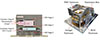 |
Figure 1. Experimental setup of CHAOS. The combined sensor head, E-Box, and baseplate have dimensions of approximately 360 mm × 260 mm × 170 mm and a mass of approximately 5 kg. |
All detector signals are processed by the analog and digital electronics within a separate electronics box (E-Box). The number of readout channels for the whole instrument is limited to 18. Table 1 summarizes the individual channels. Operating the PMT requires a high voltage of around 800 V, which poses a significant risk of corona discharges in low-pressure environments such as those encountered during the BEXUS balloon flight. The sensor head and the E-Box are therefore placed inside an aluminum pressure housing of 5.5 mm thickness, which also shields the sensors from external light. In space, such a pressure housing is not needed, and its removal would lower the minimum detectable particle energies. For thermal control during the BEXUS balloon flight, the instrument and its pressure housing were placed inside a polystyrene insulation box and wrapped in reflective foil. This insulation was not used during the measurements at the CERF facility. The combined sensor head, E-Box, and baseplate (see Fig. 1) have dimensions of approximately 360 mm × 260 mm × 170 mm and a mass of approximately 5 kg.
Calibration factors and Level-1 trigger thresholds for the readout channels of CHAOS. The calibration factors for Scintillator Stage D are given for a BGO temperature of 0°C. The calibration factors are denoted as HG for high gain, LG for low gain, and SG for single gain. Note that the given Level-1 trigger threshold for Channel B was used for the data acquisition of the readout electronics, not the data evaluation described in Section 4. If applicable, the Level-1 trigger thresholds are given as high gain/low gain.
2.1 SSD Stages A, C, and E
The SSD Stages A, C, and E provide measurements of the energy deposited by charged particles as they pass through them. All SSDs are passivated implanted planar silicon detectors that have circular detector faces with a diameter of approximately 36.49 mm and a thickness of approximately 300 μm. The detector surfaces of the SSDs are split into three ring-shaped segments surrounded by an outer guard ring. For the readout of SSD Stages A and C, the two inner detector segments are combined into a single readout segment with a radius of 17.4 mm, respectively. These segments are called A1 and C1. The outer segments are called A2 and C2. For each of the four SSDs of SSD Stage E, all three segments are combined into a single readout segment, which are called E0, E1, E2, and E3. All readout segments are read out with two different amplification factors, denoted as high and low gain, except for E1, E2 and E3, which use single-gain readout. This results in a total of 13 SSD channels. The high-gain channels are used for the detection of electrons and protons, while the low-gain channels are needed for the detection of heavier particles, which have a higher energy loss.
2.2 Cherenkov Stage B
The Cherenkov Stage B is a velocity threshold detector and utilizes the energy-dependent photon emission of different particle species due to the Cherenkov effect (Cherenkov 1934, 1937). Its centerpiece is a block of silicon dioxide aerogel (SiO2) with dimensions of 62 mm × 62 mm × 40 mm and a refractive index n ≈ 1.05. Due to its air-filled pores, the aerogel is very fragile and has a low mass density ρ ≈ 0.18 g/cm3 (Tabata et al. 2016). If a charged particle passes through a dielectric medium such as the aerogel with a velocity v greater than the local phase velocity of light c *, Cherenkov photons are emitted. This translates into Condition 1 with the speed of light c and the Lorentz beta β = v/c (Frank & Tamm 1937):
 (1)
(1)
Different particle species reach the local phase velocity of light c* at different kinetic energies due to their different masses. For example, protons have approximately 1836 times the mass of electrons and therefore need larger kinetic energies to produce Cherenkov photons. For the aerogel of CHAOS, the local phase velocity of light is c* ≈ 2.855 × 10⁸ m/s or around 95% of the speed of light in vacuum. This corresponds to threshold energies of approximately 2.1 GeV for protons and 1.2 MeV for electrons.
The total number of Cherenkov photons produced per unit path length dN/dx in the wavelength interval from λ 1 to λ 2 can be calculated by integrating the Frank-Tamm formula (Beringer et al. 2012) over the given wavelength interval (Eq. 2):
 (2)
(2)
Z is the charge number of the traversing particle and α the fine-structure constant. Equation (2) assumes a constant permeability μ and a constant refractive index n for the dielectric medium. Figure 2 shows this equation for different particle species. The different threshold energies at which the production of Cherenkov photons starts are clearly visible. It has to be noted that undoped silica aerogel does not produce scintillation photons because its band gap is too large.
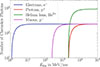 |
Figure 2. Number of Cherenkov photons produced by electrons, protons, helium ions and muons that pass through a 40 mm thick block of aerogel as function of their kinetic energy E kin. The calculations were made for the wavelength interval from λ 1 = 300 nm to λ 2 = 500 nm under the assumption of a constant refractive index n = 1.05 by integrating the Frank-Tamm formula (Eq. 2) over the given wavelength interval. |
Cherenkov Stage B includes a Hamamatsu PMT of type R1924A-7001, which has ten dynode stages over which a high voltage of approximately 800 V is applied. The PMT is needed to convert the few photons produced inside the aerogel into a detectable charge pulse. The wavelength interval from λ 1 = 300 nm to λ 2 = 500 nm used in Figure 2 was chosen in accordance with the wavelength interval in which the PMT shows its highest sensitivity. Still, this corresponds to the production of only approximately 227 photons in the 40 mm thick aerogel block of CHAOS by particles that have a charge number Z = 1, as well as sufficient kinetic energy. A lot of photons are absorbed within the aerogel, which stresses the necessity of a PMT. To further minimize the loss of initial photons, the aerogel is wrapped in multiple layers of Merck Millipore membrane filter material, which is fixed with Teflon tape. Millipore is used because it is highly reflective. Cherenkov Stage B uses a single-gain readout, resulting in a single channel.
2.3 Scintillator Stage D
In addition to the SSDs, Scintillator Stage D also measures energy losses of incident charged particles. This detector stage takes heritage from the scintillator of the HET (Rodríguez-Pacheco et al. 2020) onboard SolO (Müller et al. 2020). It uses a hexagonal BGO (Bi4Ge3O12) crystal in which charged particles create scintillation light if they pass through it. The number of scintillation photons produced is, in general, proportional to the energy deposition in the BGO crystal. A correction for nonlinearities due to ionization quenching is not applied because such a correction is only needed for heavy ionizing particles (Birks 1951). Possible contributions of Cherenkov photons to the light yield in Scintillator Stage D can also be neglected (Roncali et al. 2019).
At this point, it is important to highlight that the amount of photons produced is also dependent on the temperature of the crystal. Therefore, a temperature calibration was performed, which is discussed in Section 2.5. Each of the six side faces of the crystal has a length of around 52 mm, while the thickness of the crystal is 20 mm, which makes it larger than the one used in the HET. The BGO crystal is very heavy with a mass density ρ = 7.13 g/cm3, especially compared with the aerogel. Similar to the aerogel, the BGO crystal is wrapped in Merck Millipore membrane filter material and Teflon tape to prevent photons from escaping. Six Si-PIN S3590-09 photodiodes2 with sensitive areas of 10 mm × 10 mm are glued to the side faces of the crystal to measure the light output. The photodiodes are split into two groups of three diodes, which are called D1 and D2 and use dual gain readout. Hence, Scintillator Stage D has four channels in total.
2.4 Readout electronics and data processing
The readout electronics and data processing of CHAOS are based on the Electron Proton Telescope (EPT) and the HET (Rodríguez-Pacheco et al. 2020) onboard SolO (Müller et al. 2020) as well as previous balloon missions from Kiel University. If the detector stages register a particle, fast charge pulses are emitted, which are then amplified by charge sensitive amplifiers3. These integrator circuits collect the generated charge carriers in a capacitor that discharges with a time constant of 100 μs. Subsequently, the resulting voltage steps are converted into unipolar pulses by shapers with pole-zero correction. The shapers also provide additional gain. RC filters are applied before the shaper outputs are sampled by Analog-to-Digital Converters (ADCs) at a rate of 3 million samples per second. For each step of the ADC clock, a field-programmable gate uses a subset of 16 samples from 64 stored samples of the ADC outputs to calculate the pulse heights. For each of the 18 readout channels, the pulse height is compared to a configurable threshold value. If the threshold value is exceeded, that channel is considered to be triggered. This is a so-called Level-1 trigger. The Level-1 trigger thresholds can be found in Table 1. CHAOS does not write data based on Level-1 triggers alone. For that, so-called Level-2 triggers are used, where a predefined combination of channels has to be triggered. The Level-2 triggers can be found in Table 2.
Level-2 triggers used by the readout electronics of CHAOS. For the coincidence logic, it is not important whether a high-gain or a low-gain channel was triggered.
2.5 Calibration
The calibration of the SSDs was performed on ground with a 207Bi source by identifying the Compton edges of 569.7 keV γ-rays in the measured spectra. With this calibration, the pulse heights of the SSDs can be converted into deposited energies assuming a linear relationship and no offset.
For Scintillator Stage D, multiple separate calibrations were performed in order to calculate the energy deposited in the BGO crystal. First, the photodiodes glued to the BGO crystal were calibrated on ground similar to the SSDs to correct for potential differences in their pulse heights. Since the number of scintillation photons produced in the BGO crystal does not only depend on the deposited energy but also on the temperature of the crystal (Melcher et al. 1985), an additional temperature calibration was performed in a thermal vacuum chamber by measuring GCR muons. GCR muons were used because the 207Bi source does not cause signals that are large enough to be detected by Scintillator Stage D. These two calibrations allow for the correct calculation of the deposited energy in Scintillator Stage D. Finally, a so-called in-flight calibration has been performed by comparing the energy loss of minimum ionizing particles (MIPs) in the simulation results described in Section 3.1 with the signals caused by MIPs in Scintillator Stage D during the BEXUS balloon flight (see Sect. 3.2). This in-flight calibration gives the energy deposited in the BGO crystal. More information on the MIPs can be found in Section 5.
For further data evaluation in this paper, the on-ground calibration is used for SSD Stages A, C, and E, while the in-flight calibration is used for Scintillator Stage D. The pulse heights of Cherenkov Stage B can be converted into a photon number by comparing them to the simulation results. This is discussed in more detail in Section 4.
All calibration factors are summarized in Table 1.
3 Data sets
In this paper, three different data sets are used to demonstrate how different particle species can be identified within the measurements of CHAOS. The data sets are described in the following.
3.1 Simulation data
Using the Monte Carlo-based simulation toolkit GEANT44 (Agostinelli et al. 2003; Allison et al. 2006, 2016), simulation data were generated to compare them with the measurement data of CHAOS. The detector model of CHAOS for the simulation consisted of the different detector stages with a box of aluminum placed around them to model the shielding by the pressure housing. This box had a thickness of 5.5 mm. Additional aluminum plates of 1.0 mm thickness were placed directly above and below Cherenkov Stage B to model the aerogel enclosure, which can be seen in Figure 1. Electrons with energies from 0.5 MeV to 10 GeV and protons, muons, and helium nuclei with energies from 10 MeV/nuc to 10 GeV/nuc were simulated. Positrons and antimuons were simulated as well, but they are not shown in this paper because their behavior in the instrument is not significantly different from that of their antiparticles. For each particle type, 108 particles were simulated with an E −1 energy spectrum. The particles were shot onto the detector model from a circular source with a radius of 27 mm, which was placed 1 cm above SSD Stage A. This particle source was considered sufficient, as only particles that trigger the AC coincidence (see Sect. 2) are of interest. Therefore, only particles from a small field of view are considered. To ensure an isotropic flux for the incident particles, their angular distribution followed a cosine law. The energy losses of the particles in the detector stages were computed using the particle interaction processes that are already implemented in GEANT4. However, the number of Cherenkov photons produced in the aerogel of Cherenkov Stage B was calculated with the Frank-Tamm formula (Eq. 2) in the wavelength interval from λ 1 = 300 nm to λ 2 = 500 nm, which was chosen to match the spectral sensitivity of the PMT. The photon yield was calculated for each step that a particle took inside the aerogel during the simulation. Photons produced by secondary particles in the simulation were attributed to the primary simulated particle, as there is no way to distinguish the photons in the real measurements.
3.2 Flight data
On October 2, 2024, CHAOS was launched on a stratospheric balloon from Esrange Space Center in northern Sweden as part of the BEXUS 35 mission. After the ascent phase, the balloon floated in an altitude range of 26 km to 27 km for around 3.5 hours, before the balloon was cut off and CHAOS returned to the ground. The flight data set is taken from the so-called floating phase between ascent and cutoff. During this time, CHAOS was able to measure particles from primary GCRs (Blasi 2013; Grenier et al. 2015) and secondary particles created in extensive air showers (EAS; Engel et al. 2011). Most importantly, electrons and protons were measured, which can be used to demonstrate the capabilities of Cherenkov Stage B. The instrument was mounted on the balloon gondola with SSD Stage A facing upwards. As will be discussed in more detail in Section –5, a muon contribution is present in the flight data. These muons are secondary particles from EASs and contaminate the proton measurements. Furthermore, it has to be noted that antiparticles of the aforementioned particles (e.g. positrons and antimuons) are also part of the charged particle environment in the atmosphere (Engel et al. 2011). In this paper, antiparticles are always implicitly included when discussing a specific particle type, as they interact in the same way with the detector stages of CHAOS as their counterparts.
3.3 CERF data
Further measurements were performed at the CERN-EU high-energy Reference Field (CERF; Mitaroff & Silari 2002) in May 2025 (Mitaroff & Silari 2002). The CERF facility provides a neutron reference field that resembles the neutron field at commercial flight altitudes. However, the provided radiation field also consists of photons, muons, pions, electrons, and protons. It can therefore be used to test Cherenkov Stage B. Again, the radiation environment also includes the corresponding antiparticles (Pozzi & Silari 2020). To create the radiation field, a positive hadron beam is stopped in a copper target, generating secondary particles that subsequently travel through one of two roof shields. These shields are made up of either iron or concrete and produce the final radiation field. Due to pion decay within the beam line, a significant muon background is present at the measurement locations above the roof shields. To minimize the muon contamination, CHAOS was positioned at one of the additional measurement positions beside the beam line, where a reduced muon background was expected. These positions are behind a concrete wall of 80 cm thickness, which serves as the necessary shielding to produce the radiation field (Mitaroff & Silari 2002). CHAOS was oriented horizontally, so that the telescope defined by the detector stages was parallel to the ground, with SSD Stage A facing the concrete wall.
4 Threshold of Cherenkov Stage B
To differentiate between particles that produced photons in Cherenkov Stage B and those that did not, a threshold value has to be defined for the pulse heights of the detector stage. Figure 3 shows histograms of the pulse heights for Cherenkov Stage B for the flight data (blue), the CERF data (green), and the combined simulation data of electrons and protons (orange). The left panel shows the histograms for the complete data sets, and the right panel shows particles in AC coincidence. Particles in this coincidence deposited energy in both SSD Stages A and C, which are placed before and after Cherenkov Stage B. This way, it is ensured that the particles also passed through the aerogel of Cherenkov Stage B, so that the detector stage can be used for further data evaluation.
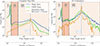 |
Figure 3. Pulse height histograms for Cherenkov Stage B for the flight data (blue), the CERF data (green), and the combined simulation data of electrons and protons (orange). The abscissae show the pulse heights in the unit of mV for the flight and CERF data and the number of photons for the simulation data. For better comparison of the different data sets, the Z = 1 peak of the simulation data was aligned with the corresponding peak in the flight data, which is marked with the blue dotted line. Three regions are highlighted, with boundaries marked by black dashed lines at 18 mV and 45 mV, corresponding to 17 photons and 42 photons for the simulation data, respectively. For the ordinates, the registered counts per bin are shown (note the different axis ranges). The left panel shows the complete data sets, while the right panel uses the AC coincidence. In this coincidence, only particles that deposited energy in both SSD Stages A and C are considered, which implies that the particles must have passed through Cherenkov Stage B. |
The histograms in Figure 3 are divided into three regions. We say that Cherenkov Stage B did not trigger for pulse heights in Region I and triggered for pulse heights in Region III. For Region II, no clear statement can be made, which is explained later on. The boundaries of these regions at 18 mV and 45 mV were chosen by visually examining the flight data and correspond to 17 photons and 42 photons for the simulation data, respectively. The conversion was done by fitting a Gaussian distribution to the peak in Region III of the flight data, which was found at 240 mV. It is assumed that the peak is caused by particles with a charge number Z = 1. In Section 2.2, it was described that these particles are expected to produce approximately 227 photons in Cherenkov Stage B. The ratio of these two numbers can be used to convert pulse heights in mV into photon numbers, and allow the comparison of the flight and CERF data with the simulation data.
Pulse heights in Region I are interpreted as particles that did not trigger Cherenkov Stage B and were therefore slower than the phase velocity of light c * in the aerogel and produced no Cherenkov photons. Thus, only electrical noise is observed for these particles in the flight and CERF data, which leads to peaks at around 15 mV in Region I. Such a peak is not present in the simulation data.
Region II contains pulse heights that cannot be clearly attributed to particles that either triggered or did not trigger Cherenkov Stage B. Data with pulse heights in this region are therefore ignored for all further data evaluation if Cherenkov Stage B is used. Both the flight and CERF data show a peak in Region II, which is most prominent when looking at the complete data sets. It is assumed that these are the single-electron peaks (Dossi et al. 2000), which are caused by single electrons randomly leaving the photocathode of the PMT due to, for example, thermal emission. No such peak is visible in the simulation data, as it simulates only the amount of photons produced by the Cherenkov effect.
The pulse heights in Region III are attributed to particles that were faster than the phase velocity of light c * in the aerogel and triggered Cherenkov Stage B by producing Cherenkov photons. Each data set shows the expected peak for particles with a charge number of Z = 1 in this region. It can be seen that these peaks are very broad, making it hard to clearly distinguish them from the single-electron peaks in Region II. This overlap is the reason why pulse heights in Region II cannot be clearly attributed to particles that triggered or did not trigger Cherenkov Stage B. The width of the Z = 1 peaks can be explained using Figure 2. The Frank-Tamm formula does not produce a step function with a sharp cutoff for the number of produced Cherenkov photons. Instead, it results in a rising edge at the threshold energies, causing the Z = 1 peaks to smear out towards lower pulse heights. This effect is most visible in the simulation data. Another factor contributing to the peak width is the statistical nature of the amplification process of the PMT.
A notable feature is the slower drop-off of the flight data at large pulse heights in comparison to the CERF data. This could be attributed to high-energy helium ions, which are only present in the flight data and trigger Cherenkov Stage B. With their charge number of Z = 2, they are expected to produce Z 2 = 4 times the amount of Cherenkov photons compared with particles with Z = 1 (see Fig. 2).
It has to be noted that further investigations of the simulation data showed a negligible amount of secondary electrons as a result of primary particles interacting with the material of the instrument. Depending on the traveled distance in the aerogel, these secondary electrons produced different numbers of Cherenkov photons and contributed to events in all three regions of Figure 3. They also caused the steps in the simulation data at approximately 500 produced photons in both panels of Figure 3.
5 Particle identification
To visualize the different data sets and identify different particle species within them, the dE/dx − dE/dx method can be employed (e.g. Marquardt & Heber 2019). It uses the energy losses in two detectors of a particle telescope and compares them with each other. In Figure 4, the dE/dx − dE/dx method is applied to the simulation data (see Sect. 3.1), which used an E−1 energy spectrum. The energy losses in SSD Stage C are shown as a function of the energy losses in Scintillator Stage D, creating a two-dimensional histogram. Here, the ACD coincidence is used, which means that only particles that deposited energy in SSD Stages A and C, as well as Scintillator Stage D, are visualized. As a consequence, the particles must also have passed through Cherenkov Stage B. For the simulation data set, all particles entered the sensor head from above and consequently passed through SSD Stage C before Scintillator Stage D. To indicate where a specific particle type would appear within the histogram, contour lines are given. They are based on histograms of simulation data (see Sect. 3.1) for the individual particle types and lie at the respective 5% levels of the maximum histogram values. The sharp edges at low energy losses in the visualized data are due to the trigger thresholds of the detector stages.
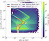 |
Figure 4. dE/dx − dE/dx method applied to simulation data of electrons, protons, helium ions, and muons similar to Panel a in Figure 5. A two-dimensional histogram of particles in ACD coincidence is shown, which means that the visualized particles deposited energy in SSD Stages A and C as well as Scintillator Stage D. Therefore, the particles also passed through Cherenkov Stage B. The abscissae show the energy loss in Scintillator Stage D while the ordinates show the energy loss in SSD Stage C. For SSD Stage C, the maximum value of the signals measured by the two readout segments of the SSD is taken, as a particle can only deposit energy in one readout segment while passing through SSD Stage C. Individual histograms were created separately for each simulated particle type and added afterwards to create the depicted combined histogram. Additionally, contour lines are shown to indicate where each particle type appears within the histogram. The contour lines are based on the histograms created for the individual simulated particle types and lie at the respective 5% levels of the maximum histogram values. |
It can be seen that ions form characteristic tracks in the histogram. To understand these tracks, the proton track is discussed in the following. From simulations (see Sect. 3.1), it is known that protons need an initial kinetic energy of approximately 50 MeV to reach Scintillator Stage D and thus penetrate all previous detector stages. These protons deposit a fraction of their kinetic energy in SSD Stage C and stop in Scintillator Stage D, where they deposit all their remaining energy of less than 10 MeV. They can be found at Position i in Figure 4. With increasing kinetic energy of the particles, the fraction of kinetic energy deposited in SSD Stage C decreases. This behavior is described by the Bethe-Bloch formula (Bethe 1930; Bloch 1933). At the same time, the remaining energy deposited in Scintillator Stage D increases. Protons with initial kinetic energies of approximately 120 MeV start to penetrate Scintillator Stage D according to the simulations and can be found at Position ii. From this energy onward, the deposited energy in Scintillator Stage D also decreases with increasing kinetic energy until Position iii is reached. Here, the minimum ionizing particle (MIP) peak can be found. The MIP peak is comprised of particles which show the lowest energy loss according to the Bethe-Bloch formula. For protons, this corresponds to initial kinetic energies of more than approximately 2 GeV. Therefore, protons with initial kinetic energies of approximately 2.1 GeV, which is their threshold energy for the production of Cherenkov photons, also fall into the vicinity of the MIP peak5.
Figure 4 shows two problems for the particle separation based on the dE/dx − dE/dx method. First of all, the MIP peak for helium ions overlaps with the proton track at Position ii. This problem can be addressed by applying other particle separation techniques, as demonstrated by Appel et al. (2018) with the Radiation Assessment Detector (RAD) or Rodríguez-Pacheco et al. (2020) with the HET. Appel et al. (2018) analyzed the ratio of energy losses in two adjacent scintillators as a function of the total energy loss in the instrument, while Rodríguez-Pacheco et al. (2020) compared the ratio of energy losses in two SSDs with the energy loss in a BGO scintillator placed between the SSDs. Similar results can be achieved with CHAOS by using the ratio of energy losses in SSD Stages C and E as a function of the energy loss in Scintillator Stage D. Ideally, SSD Stages C and E would have larger surface areas to increase statistics. A thicker BGO crystal and, therefore, larger energy loss in Scintillator Stage D would also help to separate protons and helium ions, but it would also significantly increase the mass of CHAOS. An aerogel with a refractive index of approximately 1.4 to 1.5 would also help to separate the protons and helium ions, but it would also limit the energy range in which protons can be separated from electrons.
A further problem is the contamination of the high-energy protons near the MIP peak (see Pos. iii) by electrons and muons. To remove the electrons, Cherenkov Stage B is included in the design of CHAOS. Figure 4 shows that all particles in ACD coincidence deposited more than 4 MeV in Scintillator Stage D. As a consequence, all electrons must have had kinetic energies exceeding their 1.2 MeV threshold for the production of Cherenkov photons when they passed through Cherenkov Stage B. If all particles that produced photons in Cherenkov Stage B are removed, protons with energies below 2.1 GeV are left, free from electron contamination. Still, these protons can be contaminated by muons, which need approximately 240 MeV to produce Cherenkov photons, but this is not a major concern, as the design of CHAOS is meant to be used in space one day. Here, muons are not expected (Blasi 2013; Grenier et al. 2015). Protons with kinetic energies larger than 2.1 GeV cannot be measured without electron contamination.
In Figure 5, the dE/dx − dE/dx method is applied to the simulation, flight, and CERF data in the left, center, and right columns, respectively. Similar to Figure 4, the ACD coincidence is used, and contour lines are given for orientation. The first row shows the data sets without any further restrictions except for the applied ACD coincidence. In the second row, only particles that did not trigger Cherenkov Stage B, based on the thresholds motivated in Section 4 are considered (see Region I in Fig. 3). The third row shows particles that triggered Cherenkov Stage B (see Region III in Fig. 3). Similar to Figure 4, the sharp edges of the visualized data at low energy losses are due to the trigger thresholds of the detector stages.
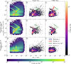 |
Figure 5. dE/dx − dE/dx plots for the simulation, flight, and CERF data (left, center and right column, respectively). Note the different color schemes for the simulation data and the actual measurements. Each panel shows a two-dimensional histogram of particles in ACD coincidence, which means that the visualized particles deposited energy in SSD Stages A and C as well as Scintillator Stage D. Therefore, the particles also passed through Cherenkov Stage B. The abscissae show the energy loss in Scintillator Stage D while the ordinates show the energy loss in SSD Stage C. For SSD Stage C, the maximum value of the signals measured by the two readout segments of the SSD is taken, as a particle can only deposit energy in one readout segment while passing through SSD Stage C. In the first row, no further restrictions except the ACD coincidence are applied to the data sets. The second row shows only particles that did not trigger Cherenkov Stage B (Region I in Fig. 3). Particles that triggered Cherenkov Stage B are shown in the third row (Region III in Fig. 3). In each panel, contour lines are shown to indicate where different particle types appear within the histograms (compare Fig. 4). |
In the first row, the particle tracks of protons and helium ions that enter the sensor head from above are visible, especially in the simulation data. Still, the populations of the different particle species overlap. Most notably, the proton MIP peaks are superimposed with electrons and muons. The CERF data (Panel c) show another particle track above the proton track, which is marked by a red arrow. Additional simulations showed that this track is caused by deuterons.
As discussed earlier, the contamination of the proton MIP peaks by electrons poses a problem, but the electrons can be removed by using Cherenkov Stage B. This is demonstrated in the second row, which only shows particles that did not trigger Cherenkov Stage B. In the simulation data (Panel d), the particle tracks for protons and helium ions are clearly visible. The proton track can also be seen in both the flight data (Panel e) and the CERF data (Panel f). There is no helium track visible in the CERF data, while in the flight data, the higher-energy part of the helium track is visible. Most importantly, there are no electrons left in the simulation data in Panel d, which is indicated by the missing contour line for electrons. No particle populations that could be attributed to electrons are visible in the flight data (Panel e) and CERF data (Panel f). Note that a muon population is left in all three panels of the second row. These are the muons with kinetic energies above approximately 240 MeV, which produce Cherenkov photons.
Particles that triggered Cherenkov Stage B are shown in the third row. The simulation data (Panel g) show the expected electrons but also the MIP protons, MIP helium ions, and MIP muons that have enough kinetic energy to produce Cherenkov photons. Similar to the simulation data (Panel g), a superposition of electrons, MIP protons and MIP muons can be observed in the flight data (Panel h). Although it is very weak, there is a feature visible in the vicinity of the contour line for helium ions. This feature is caused by MIP helium ions with kinetic energies above 2.1 GeV/nuc, which produce Cherenkov photons. The CERF data (Panel i) show a superposition of electrons, MIP protons and MIP muons as well. Compared with the flight data (Panel h), the CERF data show a more prominent electron population. Furthermore, there is no feature visible in the vicinity of the contour line for helium ions.
6 Discussion and conclusions
CHAOS was built as a prototype for the AHEPaM, which was intended to serve as a particle monitor for GCRs on ESA’s Athena mission (Nandra et al. 2013; Barret et al. 2020). This paper describes the design of CHAOS, which combines multiple SSDs and a BGO scintillator for energy loss measurements. An additional aerogel Cherenkov detector serves as a velocity threshold detector. It was successfully demonstrated that CHAOS can measure protons with kinetic energies of approximately 50 MeV up to 2.1 GeV, free from electron contamination, by applying the dE/dx − dE/dx method in combination with the aerogel Cherenkov detector. For this demonstration, measurements performed during the BEXUS 35 stratospheric balloon flight and measurements at CERN’s CERF facility were compared with GEANT4 (Agostinelli et al. 2003; Allison et al. 2006, 2016) Monte Carlo simulations. Contamination of muons in the proton measurements was observed and could not be removed. However, this does not pose a problem, as the design of CHAOS is intended for operation in space, where no muons are present (Blasi 2013; Grenier et al. 2015). Moreover, an instrument operating in space would not need a pressure housing, and its removal would lower the minimum detectable particle energy.
In the next step, particle fluxes should be derived to provide energy spectra. For this, the GEANT4 simulation model needs to be refined (e.g., inclusion of dead material such as the wrapping of the aerogel and BGO crystal) in order to calculate the response of CHAOS to particles of different types and energies. Furthermore, a measurement campaign at a beam line with well-defined energies and intensities could prove useful to validate the calibration of the instrument as well as the simulations.
The successful use of the Cherenkov detector provides valuable insights for the development of the AHEPaM as part of possible future space missions. It showed that instruments like CHAOS or the AHEPaM could indeed cover the gap in energy coverage between small instruments such as the HET (Rodríguez-Pacheco et al. 2020) and large-scale instruments such as the PAMELA (Picozza et al. 2007) and the AMS-02 (Aguilar et al. 2015), while still remaining compact instruments themselves. This is not only interesting for the measurement of GCRs but also SEPs.
Acknowledgments
We are thankful for the opportunity to develop and build CHAOS as part of the REXUS/BEXUS student programme. The REXUS/BEXUS programme is realized under a bilateral Agency Agreement between the German Aerospace Center (DLR) and the Swedish National Space Agency (SNSA). The Swedish share of the payload has been made available to students from other European countries through a collaboration with the European Space Agency (ESA). EuroLaunch, a cooperation between the Swedish Space Corporation (SSC) and the Mobile Rocket Base (MORABA) of DLR, is responsible for the campaign management and operations of the launch vehicles. Experts from DLR, SSC, ZARM and ESA provide technical support to the student teams throughout the project. REXUS and BEXUS are launched from SSC, Esrange Space Center in northern Sweden. We would like to thank all team members that are not listed as co-authors but made important contributions to the CHAOS project: Hannah Sophie Grimm, Janna Martens, Jasper Mess, Myrdin Meyer, Justus Mickausch, Clara Pittschellis, Nicolas Rohrbeck and Lars Rahn. Additionally, we thank Maximilian Brüdern, who gave us the opportunity to accompany him to CERN’s CERF facility, where we were able to perform our own measurements with CHAOS. The CHAOS design was based on developments that were performed for the Athena High-Energy Particle Monitor (AHEPaM) at Kiel University under contract No. 4000136469/21/NL/PBa with the European Space Agency (ESA). The editor thanks Grant Mitchell and an anonymous reviewer for their assistance in evaluating this paper.
Funding
We thank Kiel University for partially funding our BEXUS project.
Data availability statement
The GEANT4 simulation model, the data from the BEXUS 35 stratospheric balloon flight, and the data from the measurement campaign at CERN’s CERF facility can be found under: https://doi.org/10.5281/zenodo.18427630
References
- Agostinelli S, Allison J, Amako K, Apostolakis J, Araujo H, et al. 2003. Geant4–a simulation toolkit. Nucl Instrum Methods Phys Res A 506(3): 250–303. https://doi.org/10.1016/S0168-9002(03)01368-8. [Google Scholar]
- Aguilar M, Aisa D, Alpat B, Alvino A, Ambrosi G, et al. 2015. Precision measurement of the proton flux in primary cosmic rays from rigidity 1 GV to 1.8 TV with the alpha magnetic spectrometer on the international space station. Phys Rev Lett 114(17): 171103. https://doi.org/10.1103/PhysRevLett.114.171103. [Google Scholar]
- Allison J, Amako K, Apostolakis J, Araujo H, Dubois PA, et al. 2006. Geant4 developments and applications. IEEE Trans Nucl Sci 53(1): 270–278. https://doi.org/10.1109/TNS.2006.869826. [CrossRef] [Google Scholar]
- Allison J, Amako K, Apostolakis J, Arce P, Asai M, et al. 2016. Recent developments in Geant4. Nucl Instrum Methods Phys Res A 835: 186–225. https://doi.org/10.1016/j.nima.2016.06.125. [CrossRef] [Google Scholar]
- Appel J, Köehler J, Guo J, Ehresmann B, Zeitlin C, et al. 2018. Detecting upward directed charged particle fluxes in the mars science laboratory radiation assessment detector. Earth Space Sci 5(1): 2–18. https://doi.org/10.1002/2016EA000240. [Google Scholar]
- Barret D, Decourchelle A, Fabian A, Guainazzi M, Nandra K, et al. 2020. The Athena space X-ray Observatory and the astrophysics of hot plasma. Astron Nachr 341(2): 224–235. https://doi.org/10.1002/asna.202023782. [Google Scholar]
- Bethe H. 1930. Zur Theorie des Durchgangs schneller Korpuskularstrahlen durch Materie. Ann Phys 397(3): 325–400. https://doi.org/10.1002/andp.19303970303. [Google Scholar]
- Beringer J, Arguin J, Barnett R, Copic K, Dahl O, et al. 2012. Review of particle physics. Phys Rev D 86(1): 010001. https://doi.org/10.1103/PhysRevD.86.010001. [Google Scholar]
- Birks JB. 1951. Scintillations from organic crystals: specific fluorescence and relative response to different radiations. Proc Phys Soc A 64(10): 874. https://doi.org/10.1088/0370-1298/64/10/303. [Google Scholar]
- Blasi P. 2013. The origin of galactic cosmic rays. Astron Astrophys Rev 21: 1–73. https://doi.org/10.1007/s00159-013-0070-7. [Google Scholar]
- Bloch F. 1933. Zur Bremsung rasch bewegter Teilchen beim Durchgang durch Materie. Ann Phys 408(3): 285–320. https://doi.org/10.1002/andp.19334080303. [Google Scholar]
- Cherenkov PA. 1934. Visible light from clear liquids under the action of gamma radiation. C R (Dokl) Acad Sci URSS 2(8): 451–454. https://doi.org/10.3367/UFNr.0093.196710n.0385. [Google Scholar]
- Cherenkov PA. 1937. Visible radiation produced by electrons moving in a medium with velocities exceeding that of light. Phys Rev 52(4): 378. https://doi.org/10.1103/PhysRev.52.378. [Google Scholar]
- Dossi R, Ianni A, Ranucci G, Smirnov OJ. 2000. Methods for precise photoelectron counting with photomultipliers. Nucl Instrum Methods Phys Res A 451(3): 623–637. https://doi.org/10.1016/S0168-9002(00)00337-5. [Google Scholar]
- Engel R, Heck D, Pierog T. 2011. Extensive air showers and hadronic interactions at high energy. Annu Rev Nucl Part Sci 61(1): 467–489. https://doi.org/10.1146/annurev.nucl.012809.104544. [CrossRef] [Google Scholar]
- Fleth S, Kuehl P, Kollhoff A, Wimmer-Schweingruber RF, Heber B, et al. 2023. Anisotropies of solar energetic electrons in the MeV range measured with Solar Orbiter/EPD/HET. Astron Astrophys 676: A58. https://doi.org/10.1051/0004-6361/202345909. [Google Scholar]
- Frank I, Tamm I. 1937. Coherent visible radiation of fast electrons passing through matter. C R (Dokl) Acad Sci URSS 14(3): 109–114. https://doi.org/10.3367/UFNr.0093.196710o.0388. [Google Scholar]
- Gastaldello F, Marelli M, Molendi S, Bartalucci I, Kühl P, et al. 2022. The origin of the unfocused XMM-Newton background, its variability, and lessons learned for ATHENA. Astrophys J 928(2): 168. https://doi.org/10.3847/1538-4357/ac5403. [Google Scholar]
- Grenier IA, Black JH, Strong AW. 2015. The nine lives of cosmic rays in galaxies. Annu Rev Astron Astrophys 53: 199–246. https://doi.org/10.1146/annurev-astro-082214-122457. [Google Scholar]
- Kunow H, Müller-Mellin R, Sierks H, Wibberenz G, Raviart A, et al. 1991. The Kiel Electron Telescope on Board Ulysses. In: International Cosmic Ray Conference, Vol. 2 of International Cosmic Ray Conference, 503–506. https://ui.adsabs.harvard.edu/abs/1991ICRC....2..503K. [Google Scholar]
- Marelli M, Molendi S, Rossetti M, Gastaldello F, Salvetti D, et al. 2021. Analysis of the unconcentrated background of the EPIC pn camera on board XMM-Newton. Astrophys J 908(1): 37. https://doi.org/10.3847/1538-4357/abcfbc. [Google Scholar]
- Marquardt J, Heber B. 2019. Galactic cosmic ray hydrogen spectra and radial gradients in the inner heliosphere measured by the HELIOS Experiment 6. Astron Astrophys 625: A153. https://doi.org/10.1051/0004-6361/201935413. [Google Scholar]
- Melcher C, Schweitzer J, Liberman A, Simonetti J. 1985. Temperature dependence of fluorescence decay time and emission spectrum of bismuth germanate. IEEE Trans Nucl Sci 32(1): 529–532. https://doi.org/10.1109/TNS.1985.4336887. [Google Scholar]
- Mitaroff A, Silari M. 2002. The CERN-EU High-energy Reference Field (CERF) Facility for Dosimetry at Commercial Flight Altitudes and in Space. Radiat Prot Dosim 102(1): 7–22. https://doi.org/10.1093/oxfordjournals.rpd.a006075. [Google Scholar]
- Müller D, St Cyr OC, Zouganelis I, Gilbert HR, Marsden R, et al. 2020. The Solar Orbiter mission – Science overview. Astron Astrophys 642: A1. https://doi.org/10.1051/0004-6361/202038467. [CrossRef] [EDP Sciences] [Google Scholar]
- Nandra K, Barret D, Barcons X, Fabian A, Herder JWd, et al. 2013. The hot and energetic universe: A white paper presenting the science theme motivating the Athena+ mission. Preprint [https://arxiv.org/abs/1306.2307] [Google Scholar]
- Picozza P, Galper A, Castellini G, Adriani O, Altamura F, et al. 2007. PAMELA–A payload for antimatter matter exploration and light-nuclei astrophysics. Astropart Phys 27(4): 296–315. https://doi.org/10.1016/j.astropartphys.2006.12.002. [Google Scholar]
- Pozzi F, Silari M. 2020. The CERN-EU high-energy Reference Field (CERF) facility: New FLUKA reference values of spectral fluences, present and newly proposed operational quantities. Nucl Instrum Methods Phys Res A 979: 164477. https://doi.org/10.1016/j.nima.2020.164477. [Google Scholar]
- Reames DV. 2023. Review and outlook of solar energetic particle measurements on multispacecraft missions. Front Astron Space Sci 10: 1254266. https://doi.org/10.3389/fspas.2023.1254266. [Google Scholar]
- Rodríguez-Pacheco J, Wimmer-Schweingruber R, Mason G, Ho G, Sánchez-Prieto S, et al. 2020. The Energetic Particle Detector – Energetic particle instrument suite for the Solar Orbiter mission. Astron Astrophys 642: A7. https://doi.org/10.1051/0004-6361/201935287. [Google Scholar]
- Roncali E, Il Kwon S, Jan S, Berg E, Cherry SR. 2019. Cerenkov light transport in scintillation crystals explained: realistic simulation with GATE. Biomed Phys Eng Express 5(3): 035033. https://doi.org/10.1088/2057-1976/ab0f93. [Google Scholar]
- Sullivan J. 1971. Geometrical factor and directional response of single and multi-element particle telescopes. Nucl Instrum Methods 95(1): 5–11. https://doi.org/10.1016/0029-554X(71)90033-4. [CrossRef] [Google Scholar]
- Tabata M, Adachi I, Hatakeyama Y, Kawai H, Morita T, et al. 2016. Large-area silica aerogel for use as Cherenkov radiators with high refractive index, developed by supercritical carbon dioxide drying. J Supercrit Fluids 110: 183–192. https://doi.org/10.1016/j.supflu.2015.11.022. [Google Scholar]
For SSD Stages A, C, and E, the charge pulses come directly from the SSDs. In the case of Cherenkov Stage B, the charge pulses come from the PMT and for Scintillator Stage D, they are emitted from the photodiodes.
Version: 10.5.1, Physics list: QGSP_BERT_HP_EMZ.
Technically, a proton needs an initial kinetic energy larger than 2.1 GeV to produce Cherenkov photons because it loses some of its energy while passing through the aluminum pressure housing, SSD Stage A, and the aluminum aerogel enclosure. For the production of Cherenkov photons, a kinetic energy of 2.1 GeV has to be left when the proton reaches the aerogel of Cherenkov Stage B. However, for protons that fall into the MIP peak, the energy loss due to shielding is negligible according to the Bethe-Bloch formula. This holds for MIPs of all particle species discussed in this paper.
Cite this article as: Pohley A, Ebeling H, Borneth P, Böttcher SI, Kühl P, et al. 2026. Bridging the measurement gap between MeV and GeV particles in space: Design and first results of the CHerenkov Atmospheric Observation System (CHAOS). J. Space Weather Space Clim. 16, 21. https://doi.org/10.1051/swsc/2026016.
All Tables
Calibration factors and Level-1 trigger thresholds for the readout channels of CHAOS. The calibration factors for Scintillator Stage D are given for a BGO temperature of 0°C. The calibration factors are denoted as HG for high gain, LG for low gain, and SG for single gain. Note that the given Level-1 trigger threshold for Channel B was used for the data acquisition of the readout electronics, not the data evaluation described in Section 4. If applicable, the Level-1 trigger thresholds are given as high gain/low gain.
Level-2 triggers used by the readout electronics of CHAOS. For the coincidence logic, it is not important whether a high-gain or a low-gain channel was triggered.
All Figures
|
Figure 1. Experimental setup of CHAOS. The combined sensor head, E-Box, and baseplate have dimensions of approximately 360 mm × 260 mm × 170 mm and a mass of approximately 5 kg. |
| In the text | |
|
Figure 2. Number of Cherenkov photons produced by electrons, protons, helium ions and muons that pass through a 40 mm thick block of aerogel as function of their kinetic energy E kin. The calculations were made for the wavelength interval from λ 1 = 300 nm to λ 2 = 500 nm under the assumption of a constant refractive index n = 1.05 by integrating the Frank-Tamm formula (Eq. 2) over the given wavelength interval. |
| In the text | |
|
Figure 3. Pulse height histograms for Cherenkov Stage B for the flight data (blue), the CERF data (green), and the combined simulation data of electrons and protons (orange). The abscissae show the pulse heights in the unit of mV for the flight and CERF data and the number of photons for the simulation data. For better comparison of the different data sets, the Z = 1 peak of the simulation data was aligned with the corresponding peak in the flight data, which is marked with the blue dotted line. Three regions are highlighted, with boundaries marked by black dashed lines at 18 mV and 45 mV, corresponding to 17 photons and 42 photons for the simulation data, respectively. For the ordinates, the registered counts per bin are shown (note the different axis ranges). The left panel shows the complete data sets, while the right panel uses the AC coincidence. In this coincidence, only particles that deposited energy in both SSD Stages A and C are considered, which implies that the particles must have passed through Cherenkov Stage B. |
| In the text | |
|
Figure 4. dE/dx − dE/dx method applied to simulation data of electrons, protons, helium ions, and muons similar to Panel a in Figure 5. A two-dimensional histogram of particles in ACD coincidence is shown, which means that the visualized particles deposited energy in SSD Stages A and C as well as Scintillator Stage D. Therefore, the particles also passed through Cherenkov Stage B. The abscissae show the energy loss in Scintillator Stage D while the ordinates show the energy loss in SSD Stage C. For SSD Stage C, the maximum value of the signals measured by the two readout segments of the SSD is taken, as a particle can only deposit energy in one readout segment while passing through SSD Stage C. Individual histograms were created separately for each simulated particle type and added afterwards to create the depicted combined histogram. Additionally, contour lines are shown to indicate where each particle type appears within the histogram. The contour lines are based on the histograms created for the individual simulated particle types and lie at the respective 5% levels of the maximum histogram values. |
| In the text | |
|
Figure 5. dE/dx − dE/dx plots for the simulation, flight, and CERF data (left, center and right column, respectively). Note the different color schemes for the simulation data and the actual measurements. Each panel shows a two-dimensional histogram of particles in ACD coincidence, which means that the visualized particles deposited energy in SSD Stages A and C as well as Scintillator Stage D. Therefore, the particles also passed through Cherenkov Stage B. The abscissae show the energy loss in Scintillator Stage D while the ordinates show the energy loss in SSD Stage C. For SSD Stage C, the maximum value of the signals measured by the two readout segments of the SSD is taken, as a particle can only deposit energy in one readout segment while passing through SSD Stage C. In the first row, no further restrictions except the ACD coincidence are applied to the data sets. The second row shows only particles that did not trigger Cherenkov Stage B (Region I in Fig. 3). Particles that triggered Cherenkov Stage B are shown in the third row (Region III in Fig. 3). In each panel, contour lines are shown to indicate where different particle types appear within the histograms (compare Fig. 4). |
| In the text | |
Current usage metrics show cumulative count of Article Views (full-text article views including HTML views, PDF and ePub downloads, according to the available data) and Abstracts Views on Vision4Press platform.
Data correspond to usage on the plateform after 2015. The current usage metrics is available 48-96 hours after online publication and is updated daily on week days.
Initial download of the metrics may take a while.