| Issue |
J. Space Weather Space Clim.
Volume 8, 2018
Developing New Space Weather Tools: Transitioning fundamental science to operational prediction systems
|
|
|---|---|---|
| Article Number | A22 | |
| Number of page(s) | 14 | |
| DOI | https://doi.org/10.1051/swsc/2018017 | |
| Published online | 17 April 2018 | |
Research Article
Geomagnetic storm forecasting service StormFocus: 5 years online
1
Skolkovo Institute of Science and Technology,
Moscow, Russia
2
Space Research Institute,
Moscow, Russia
* Corresponding author: This email address is being protected from spambots. You need JavaScript enabled to view it.
Received:
24
May
2017
Accepted:
18
February
2018
Abstract
Forecasting geomagnetic storms is highly important for many space weather applications. In this study, we review performance of the geomagnetic storm forecasting service StormFocus during 2011–2016. The service was implemented in 2011 at SpaceWeather.Ru and predicts the expected strength of geomagnetic storms as measured by Dst index several hours ahead. The forecast is based on L1 solar wind and IMF measurements and is updated every hour. The solar maximum of cycle 24 is weak, so most of the statistics are on rather moderate storms. We verify quality of selection criteria, as well as reliability of real-time input data in comparison with the final values, available in archives. In real-time operation 87% of storms were correctly predicted while the reanalysis running on final OMNI data predicts successfully 97% of storms. Thus the main reasons for prediction errors are discrepancies between real-time and final data (Dst, solar wind and IMF) due to processing errors, specifics of datasets.
Key words: Solar wind / magnetic field / storm / forecasting / validation
© T. Podladchikova et al., Published by EDP Sciences 2018
 This is an Open Access article distributed under the terms of the Creative Commons Attribution License (http://creativecommons.org/licenses/by/4.0), which permits unrestricted use, distribution, and reproduction in any medium, provided the original work is properly cited.
1 Introduction
When the southward interplanetary magnetic field (IMF) embedded in the solar wind affects the Earths magnetic field during several hours, a substantial energy is transferred into the magnetosphere. The entire magnetosphere becomes disturbed and this state is characterized as “geomagnetic storm” (e.g., Gonzalez et al., 1994). The common measure of intensity of a geomagnetic storm is Dstp geomagnetic index—a depression of equatorial geomagnetic field, associated primarily with the magnetospheric ring current. The strength of geomagnetic storm is characterized by the maximum negative value of the index, which is denoted hereafter as Dstp.
Operational forecasting of geomagnetic storms is highly important for space weather applications. The geomagnetic storms can be predicted qualitatively, when the large scale events on the Sun (flares, CMEs or coronal holes) are detected. The propagation time of solar wind from Sun to Earth is about 1–5 days, creating the natural time interval for such predictions. However, the magnetic structure of an interplanetary perturbation (magnetic cloud or stream interface), in particular IMF Bz profile (hereafter GSM frame of reference is used), which is of prime importance for the magnetospheric dynamics, can not be determined for now from solar observations. Thus, detailed forecast of a storm strength several days in advance is currently impossible.
Quantitative geomagnetic predictions can be performed using the measurements of interplanetary magnetic field and solar wind by a spacecraft in the libration point L1. The difference in the propagation time from L1 to Earth between radio signal and solar wind is typically one hour, providing the chance for the short-term forecast. Intrinsic solar wind and IMF variations can deteriorate the quality of such a forecast, changing the input on the way from L1 to the magnetosphere. However, as shown in Petrukovich et al. (2001), the relatively large-scale storm-grade interplanetary disturbances are well preserved between L1 and Earth, while the smaller-scale substorm-grade disturbances indeed can change substantially. The gap between two currently available methods (solar and L1) might be filled, in particular, by developing the methods of advance forecasting several hours ahead of available solar wind data.
The modeling of Dst index is relatively well performed using IMF and solar wind as input. Current approaches can be, in general, divided into several groups. The first variant is based on the statistical dependence of the Dst minima during storms on geoefficient solar wind parameters (southward magnetic field or coupling functions) (e.g., Akasofu, 1981; Petrukovich and Klimov, 2000; Yermolaev and Yermolaev, 2002; Gonzalez and Echer, 2005; Yermolaev et al., 2005; Kane and Echer, 2007; Echer et al., 2008; Mansilla, 2008; Yermolaev et al., 2010; Echer et al., 2013; Rathore et al., 2014).
The second approach is based on a first-order differential equation of Dst index evolution depending on geoeffective solar wind parameters (Burton et al., 1975). This approach with the later modifications (O'Brien and McPherron, 2000a,b; Siscoe et al., 2005; Nikolaeva et al., 2014) proved to be very successful and helps to model dynamics of Dst index in detail.
The third group uses various black box-type statistical models, relating the solar wind and Dst index: artificial neural networks, nonlinear auto-regression schemes, etc. (Valdivia et al., 1996; Vassiliadis et al., 1999; Lundstedt et al., 2002; Temerin and Li, 2002, 2006; Wei et al., 2004; Pallocchia et al., 2006; Sharifie et al., 2006; Zhu et al., 2006, 2007; Amata et al., 2008; Boynton et al., 2011, 2013; Caswell, 2014; Revallo et al., 2014; Andriyas and Andriyas, 2015). These models with rather complex structure are capable to extract information about the process without any prior assumptions. A detailed comparison of several such models was done for large storms (Dst<−100 nT) by Ji et al. (2012).
Finally some physics-based magnetospheric models are capable in modeling Dst (e.g., Katus et al., 2015). Rastätter et al. (2013) compared statistical and physics-based models and also presented a nice review of approaches.
Operational use of such Dst models with the L1 real-time solar wind naturally provides a forecast with the lead time of the order of one hour. Forecasting Dst several hours ahead (of available solar wind) is a more challenging topic. One can generate such a forecast as a simple extension of the “black-box” approach described above. Wu and Lundstedt (1997) and Sharifie et al. (2006) used the neural network and local linear neuro-fuzzy models, however these results were not presented in sufficient details. A similar approach was used to predict Kp ahead of solar wind by Wing et al. (2005). Bala and Reiff (2012) used an artificial neural network to forecast several indices via the empirical estimate of the Earth's polar cap potential. Frequently authors also discuss the “one step ahead” forecast (Revallo et al., 2014).
Considering approaches to multi-hour forecasts it is helpful to keep in mind the following aspects: (1) Multi-hour forecasts require some supposition on the expected solar wind behavior. In the “black-box” type models this information is hidden from the user. However it might be essential to have full control on assumption about solar wind input. (2) Since evidently some certainty in the input is lost, it is natural to step back also in the forecast details. For example, one can formulate results in terms of thresholds. (3) The continuous Dst timeline is dominated by geomagnetically quiet intervals, thus it might be more reasonable to check the model quality only on storm events.
Several approaches were suggested, which essentially follow these ideas. Mansilla (2008) showed the straight relation between the peak Dstp and the peak value of the solar wind velocity V, and determined the time delay between Dstp and maximum negative Bz to be about several hours. However, this particular method needs statistical justification of specific forecasts. Chen et al. (2012) used bayesian model to forecast thresholds of storm strength, using the past statistics of amplitude and duration of southward IMF Bz, in particular for magnetic clouds.
Often the past measured Dst indices are also used as input, as currently the quick-look Dst is available almost immediately. In a case of delay in quick-look Dst, the index can be reasonably well reconstructed using solar wind (e.g., Lundstedt et al., 2002; Wei et al., 2004; Sharifie et al., 2006; Zhu et al., 2007).
In the first publication (Podladchikova and Petrukovich, 2012) we developed the prediction technique of the geomagnetic storm peak strength Dstp at the first relevant signs of storm-grade input in the solar wind. It uses the extrapolation of the Burton-type Dst model with the constant solar wind input to provide the forecast several hours ahead of available solar wind data. The method essentially relies on the relative persistency of large-scale storm-grade solar wind and IMF structures and on the cumulative nature of Dst index, partially integrating out input variations. In fact, the stronger is the expected storm, the easier is such forecast. On the basis of the proposed technique a new online geomagnetic storm forecasting service was implemented in 2011 at SpaceWeather.Ru. Since 2017, we adopted the name StormFocus. In this study, we review performance of StormFocus during more than five years of operation 2011–2016 and verify the algorithm thresholds and other calculation details. The solar maximum of the cycle 24 is rather weak, so most of new statistics are rather moderate storms. We also analyze the origins of the observed errors. Besides some imperfectness of the algorithm, another major real-time error type proved to be related with the missing data and the calibration-related differences between the real-time and the final data. These latter errors are often not recognized, but actually account for a significant part of the forecast uncertainty.
More specifically, all models are designed on the final quality solar wind data, usually from the OMNI dataset, which appear with the delay of several months. OMNI data are taken from one of the several available spacecraft, verified, and shifted to Earth with a relatively complicated algorithm. The real-time data provided by NOAA are unverified, not shifted and come only from ACE (currently also from DSCOVR). As concerns Dst, the final index is available until 2010 (as of beginning 2017), while the provisional one is for 2011–2016. It might be quite different from the real-time Dst, which is used in the model (as the previous value) or which is compared with the forecast result in real-time. Our archived forecast history includes also input data and allows us to analyze these errors in detail, comparing real-time algorithm performance with the reanalysis on final OMNI and ACE/Wind spacecraft data, as well as directly comparing real-time and final input data (see also end of Sect. 2).
In Section 2, we explain our method. Section 3 describes the statistics of the forecast quality over the period of service operation July 2011–December 2016 (hereafter—the test period), including both real-time results and reanalysis using final data. Section 4 analyzes the actual error sources, including the differences between real-time and final data. Section 5 concludes with Discussion.
2 Methodology
The geomagnetic storm forecasting service StormFocus was implemented in 2011 at the website of Space Research Institute, Russian Academy of Sciences (IKI, Moscow) SpaceWeather.Ru. The full details of the prediction algorithm were in our first publication (Podladchikova and Petrukovich, 2012) and are now included in Appendix A. ACE real-time data, obtained from NOAA SWPC and real-time quicklook Dst are used as input. The prediction algorithms were initially tuned on historical data from 1995 to 2010. During this period 97 storms with (Dstp < − 100 nT) and 317 storms (−100 < Dstp < − 50 nT) were registered. The DSCOVR real-time data have been used as input, starting in October 2017. Data are averaged (boxcar) at round hours and forecasts are computed every hour. The forecasts are archived and available at http://www.iki.rssi.ru/forecast/data/Archive
The best predicted are relatively large storms with sharp turns to strong southward IMF Bz (essentially with large VBs), identified with some empirical thresholds explained in Appendix A. For such storms StormFocus provides the upper and lower limits of the future peak Dstp. These storms are called “sudden” in the terminology of Podladchikova and Petrukovich (2012). All other storms are called “gradual” storms since VBs increases with no clear step. For them the service provides the single prediction of Dstp. Our forecast is routinely updated every hour and the maximal (the most negative) prediction is kept active until storm end is signaled.
Such forecasts of storm peak values proved to be rather reliable. Errors were at the moderate level of ∼10%. Predictions were issued on average 5–6 hours before the actual peak was registered. Accuracy of predicting the time of Dstp turned out to be much worser than that of Dstp itself, thus time of storm maximum is not forecasted in our tool. Particular time of Dstp, especially for gradual storms, is likely influenced by some transient variations in solar wind or geomagnetic activity, which is in contradiction with our main hypothesis on input persistence.
Figure 1 shows the StormFocus forecast page layout for the geomagnetic storm on 6 August 2011 with the peak Dstp = − 138 nT. It includes the panels with quick-look Dst (blue), modeled Dst (cyan) using Equations ((3)–(6)), and predictions (red), with IMF Bz (green), and solar wind velocity V (black), as well as the verbal forecast. Here the real-time ACE Bz and the solar wind V are ballistically shifted forward, accounting for the L1-Earth propagation. At 21:00 UT, 5 August, 2011 the “sudden” storm was predicted with the limits from −166 to −94 nT. This prediction of peak magnitude was provided 7 hours before it was actually registered, at a moment when Dst was still positive (14 nT). Note, that the verbal warning of −52 nT storm, shown on the top of picture, corresponds to the later time 9:05 UT, when this screen-shot was generated.
In this investigation, we estimate the performance of StormFocus operation during 2011–2016. Similar to our first publication we aim at a reliable quantitative forecast. A standard approach to forecast errors specifies false warnings (errors of the first kind), misses (errors of the second kind), as well as true negatives (correct prediction of quiet interval). Since we issue forecast of storm peak magnitude every hour with the floating waiting time to the real peak, there is no consistent definition of the true negative. Moreover, a prediction of a quiet interval several hours ahead has no solid physical basis in solar wind data, since there is no guarantee, that some strong disturbance will not appear “next hour”, especially when Sun is active. Thus predictions of geomagnetically quiet intervals (though it may be of interest to some applications) are not a part of our forecast. We aim to predict only storms with Dst < − 50 nT.
In our scheme true misses are very unlikely, since L1 spacecraft is a reliable upstream monitor and no storms occur without corresponding interplanetary disturbance. However, in some cases the first satisfactory forecast could be issued rather late, well inside the developing storm. Our prime goal was to minimize false warnings (predictions of too large storms).
During quality checks we first identify all storms (below 50 nT) and their Dstp. Then we search for the earliest correct (within 25%) forecast before each observed peak. If all forecasts (before actual Dstp) are more than 25% weaker (less negative) than Dstp, the storm is considered as missed (though the forecast still may reach “correct” amplitude later than the actual Dstp was observed). If there is no correct forecast before the actual peak, but there is prediction 25% stronger (more negative) than the peak Dstp, the storm amplitude is considered overestimated (false warning). To check the usefulness of the forecast we also determine the advance time, when the successful forecast was issued (relative to actual Dstp), and Dst values at the moment of forecasts.
One more characteristic is the maximal prediction issued within a storm. The third variant of an error is identified, when this maximal prediction happens after the first correct forecast and overestimates true Dstp by more than 25%. This is called in the following “overestimated maximum prediction”.
We verify the general prediction accuracy in three variants with respect to the used data. The first variant is “true comparison” of the forecast (using ACE real-time solar wind, IMF and previous quicklook Dst) with the storm magnitude as measured by quicklook Dstp. However, from a point of view of a general user, it might be more correct to compare the forecast with actual (final) Dst. This is the second variant of our comparison. For the third variant we rerun the algorithm using final solar wind, IMF and Dst from OMNI and compare with the storm magnitude as measured with final (or provisional) Dstp. This latter approach is also known as reanalysis.
For the ACE real-time solar wind, IMF and quicklook Dst data we use our own archive for 2011–2016, which was filled in the course of operation. Final solar wind and IMF data are taken from OMNI dataset (shifted and merged data) as well as from CDAWeb for individual ACE and Wind spacecraft (not shifted original data). The final Dst is available only before 2011, thus for the later time we use provisional Dst (see also discussion in Sect. 4). In the latter text (if not explicitly stated oppositely) we use the term “final” to characterize OMNI solar wind and provisional or final Dst as opposed to the real-time data.
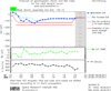 |
Fig. 1 Layout of the StormFocus forecast web page for the geomagnetic storm on 6 August 2011. |
3 Forecast statistics
In this section, we present the statistics of the forecast quality over the period of StormFocus operation July 2011–December 2016, as well as the reanalysis using the final data. The Dstp of relatively large “sudden” storms with the sufficiently sharp increase of VBs (see criteria in Appendix A (A.10) and (A.11) is forecasted with the lower and upper magnitude limits. During the test period the sudden storm criteria in real-time were activated only for 10 storms. However with the final data reanalysis there were 23 “sudden” storms. These storms were weaker than that for 1995–2010 (53 storms) used by Podladchikova and Petrukovich (2012) to design the prediction algorithms. Over the last 5 years, only three storms were below −150 nT, while for 1995–2000, 50% of such storms were with peak Dstp < − 150 nT. The “sudden” storm forecast works best for larger storms, so the conditions during last five years were not favorable in this sense.
Figure 2a shows the forecast statistics for 23 “sudden” geomagnetic storms (as determined in final data). We use real-time data input compared with the final geomagnetic index, and storms are ordered by the final Dstp (black line). The bars in Figure 2a show the forecast for 10 events, for which the “sudden” criterion was “on” in real-time, and both upper and lower forecast limits were calculated. The remaining 13 storms (marked by single points) were characterized as “gradual” in real-time, for which only one-point forecast (Appendix A) was produced. The red bar and red point indicate unsuccessful forecasts for two events. Thus, StormFocus service issued a successful forecast using the real-time input data for 21 storms, though in 9 cases it was provided with two limits and in 12 cases − with a single point. Storm forecasts were produced when the Dst index was on average weaker by 75% than the final Dstp, and in some cases the warnings were issued, when Dst index was positive (not shown here). The advance time of the real-time forecasts was 1–20 hours with the average value of about 7 hours (Fig. 2c).
Figure 2b shows the results of reanalysis on final data for 23 geomagnetic storms. The blue bars show the successful forecast of upper and lower limits of Dstp (black solid line) based on final OMNI data for 22 storms. The only red bar gives unsuccessful “overestimate” forecast, which was more than 25% stronger (more negative) than actual Dstp. Note, that this forecast was still produced in advance, and the storm was in fact detected, though the strength was overestimated. To check the usefulness of forecast we also determined the final Dst index at the issue time of Dstp forecast. On average it is weaker by 84% than the final peak Dstp.
Storms with no “sudden” criterion are categorized as gradual and their magnitude Dstp is predicted with the single number based on the three-hour forecast  (Appendix A). Five “gradual” storms had Dstp<−100 nT and 92 storms had −100 < Dstp < − 50 nT. The classification of storms is made using more reliable final Dst. Additionally, 33 storms had real-time Dstp < − 50 nT, but final Dstp > − 50 nT. These storms were also included to the forecast statistics.
Figure 3 presents the statistics of gradual storms relative to final Dstp.
With the real-time forecast, the earliest “successful” prediction (blue line in Fig. 3a) of final Dstp (black line) was produced for 109 out of 130 cases. The outliers are marked with red points, including 10 “overestimated” events, and 11 missed predictions. Cyan line shows the maximal predictions issued later within a storm. The number of overestimated maximal predictions was 37 (red points). Note that for these events the earliest forecast was successful. Mainly small storms were overestimated, when errors of a baseline are relatively more important. The storm forecasts were produced when the Dst index was on average weaker by 57% than the final Dstp, confirming the usefulness of prediction service. The advance time of the real-time forecasts was 1–20 hours with the average value of about 8 hours (Fig. 3c).
With the reanalysis using final OMNI data (Fig. 3b), 126 out of 130 storms were successfully predicted. The blue line gives the earliest prediction, which is in 25% range from final Dstp. The red points show unsuccessful missed forecast at four events. Cyan line shows the maximal predictions of Dstp issued later within a storm. The number of overestimated maximal predictions with the final data is about a half of that with real-time input (in comparison with Fig. 3a)—just 21 storms. Dst at the issue time of forecast was on average weaker by 54% than the final OMNI Dstp.
Table 1 summarizes the forecast statistics. It includes the three variants of the forecast run: real-time Dstp prediction using real-time input (“RR”), final Dstp prediction using final input (“FF”), final Dstp prediction using real-time input (“RF”). “Successful forecast” gives the number of storms with the earliest forecast of peak Dstp within 25% of the actual storm magnitude. “Overestimate” and “missed” represent the number of unsuccessful forecasts. “Overestimated maximal prediction” shows the number of overestimating forecasts issued later within a storm (when the earliest forecast was successful).
As it is clear from Table 1, over the test period our prediction algorithm performed best for the reanalysis (final input compared with final Dstp), providing 148 successful predictions of Dstp out of 153 storms. Real-time forecast compared with final Dstp resulted in 130 successes. Real-time forecast compared with real-time quicklook Dstp had 129 successes. Thus the usage of real-time input IMF, solar wind, and Dst decreased the quality of the earliest forecasts for 21 storms as compared with the final input.
In addition there were events with overestimation of maximal predictions issued later within a storm (when the earliest forecast is successful). The worst quality with respect to this criterion has the real-time forecast as compared with final index (RF variant). The number of errors was almost twice larger than for RR variant, and almost four times larger than for FF variant (42 compared with 24 and 11). The most of errors were for smaller storms (left side of Fig. 3). Most likely the main reason is the baseline difference between real-time and final Dst. In the RF-variant the forecast is computed with the real-time quicklook Dst index, while comparison is with final Dst.
All possible outcomes for the forecasts of Dstp can be described by the number of hits (successful forecast), misses, and false alarms. We can calculate the following verification measures such as the probability of detection (POD) and the ratio of overestimated forecasts (ROF) (Tab. 2).
 (1)
(1)
 (2)
The highest probability of detection (0.97) and the lowest ratio of overestimated forecast (0.007) is for FF reanalysis variant. The probability of detection decreased to 0.87 and the ratio of overestimated forecast increased to 0.04 for the real-time quicklook Dstp prediction using real-time input (RR). The numbers for RF variant remain similar to that for RR. Overestimates of the maximal forecast after successful warning are at the level of 24% for RF variant and about 10% for RR and RF variants.
(2)
The highest probability of detection (0.97) and the lowest ratio of overestimated forecast (0.007) is for FF reanalysis variant. The probability of detection decreased to 0.87 and the ratio of overestimated forecast increased to 0.04 for the real-time quicklook Dstp prediction using real-time input (RR). The numbers for RF variant remain similar to that for RR. Overestimates of the maximal forecast after successful warning are at the level of 24% for RF variant and about 10% for RR and RF variants.
Among errors in Table 1, there were in total 49 storms with some forecast errors in real-time and correct forecast with final data. These 49 errors can be definitely ascribed to real-time data errors. In the next section we analyze in detail the reasons of these differences.
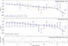 |
Fig. 2 Forecast statistics for “sudden” geomagnetic storms. (a) Storm predictions using real-time data input. (1) final Dstp; (2) the earliest prediction of both upper and lower limits of Dstp within 25% of actual storm magnitude; (3) the earliest prediction of Dstp with 3-hour forecast (not “sudden” in real-time); (4) and (5) the predictions of Dstp, which were out of 25% range from actual Dstp. (b) Storm predictions using final data input. (6) final Dstp; (7) the earliest prediction of both upper and lower limits of Dstp within 25% of actual storm magnitude; (8) the predictions of Dstp, which were out of 25% range from actual storm magnitude. (c) The advance warning time (in hours) of the Dstp forecast using real-time input. |
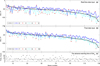 |
Fig. 3 Forecast statistics for “gradual” geomagnetic storms. (a) Storm predictions using real-time data input. (1) final Dstp; (2) the earliest prediction of Dstp within 25% of actual storm magnitude; (3) the predictions of Dstp, which were out of 25% range; (4) maximal predictions of Dstp obtained during the storm development; (5) maximal predictions out of 25% range. (b) Storm predictions using final data input. (6) final Dstp; (7) the earliest prediction of Dstp within 25%; (8) the predictions of Dstp, which were out of 25% range; (9) maximal predictions of Dstp obtained during the storm development; (10) maximal predictions out of 25% range. (c) The advance warning time (in hours) of the Dstp forecast using real-time input. |
Forecast statistics for: “RR” − real-time quicklook Dstp prediction using real-time input; “FF” − final Dstp prediction using final input; “RF” − final Dstp prediction using real-time input.
The probability of detection (POD) and the ratio of overestimated forecasts (ROF) of the earliest and maximal forecasts for the three types of the forecast run: “RR” − real-time quicklook Dstp prediction using real-time input; “FF” − final Dstp prediction using final input; “RF” − final Dstp prediction using real-time input.
4 Analysis of reasons for the decrease of the forecast quality using real-time input
Forecasting services use data available in real-time, which can be substantially different from the final calibrated data appearing later in the scientific archives. However, the forecast algorithms of Dst are designed using the final data. The forecast errors due to this factor are often overlooked, but can be equally important as those due to an algorithm imperfection. Our analysis in Section 3 shows that the number of the forecast errors is indeed much smaller if the final quality data are used. In this section we analyze specific sources of our forecast errors and the differences between real-time and final data in general.
Figure 4 shows the difference between the hourly averaged final data and real-time ACE and Dst values for the disturbed periods Dst < − 50 nT over July 2011–December 2016.
Dst index is mostly overestimated, as quick-look index available in real-time is smaller than the provisional Dst (67% of points) and for more than half of cases the difference exceeds 10 nT (Fig. 4a). This effect is responsible for the half of events under analysis (28 out of 49, Tab. 3, detailed description is below). (i.e., more negative)
It should be noted additionally that quicklook Dst is usually updated approximately half an hour after the first appearance. We do not have in hand the statistics of this change. Several years later provisional Dst is replaced by final Dst, and the scatter between these two index types is a factor of 2–3 smaller, than that for the real-time—provisional pair. Also, the final Dst is on average again weaker (more positive) than the provisional index by few nT.
Figure 5 shows the specific example of the forecast error due to the difference between quicklook and provisional Dst.
Panel (a) gives the provisional Dst and prediction of its peak Dstp using final input, as well as the same pair for the real-time data. Panel (b) shows IMF Bz from ACE real-time, final OMNI, final ACE, and final Wind. Final OMNI solar wind speed V and ACE real-time V are in panel (c). Panel (d) has the final OMNI driving parameter VBs and ACE real-time VBs.
According to real-time data the storm reached the peak Dstp of −107 nT at 6:00 UT on 27 August 2015, however the provisional Dst peak was significantly weaker reaching only −77 nT. The first “successful” real-time forecast (−81 nT) of Dstp was issued 4 hours in advance. The maximal prediction of Dstp issued later in real-time within the storm reached −102 nT, producing more accurate prediction of quicklook Dstp. However it was 32% stronger (more negative) than the actual storm strength determined by final Dstp. The primary computational reason for this overestimate was the large difference of about 20 nT between real-time and provisional Dst (the current real-time quicklook Dst index is used in forecast as initial condition). This storm has three clear intensifications. The two other were at 21:00 UT on 26 August and 21:00–23:00 UT on 27 August, and they were well predicted, since, in particular, the difference between quicklook and provisional Dst was small. At 7:00 UT on 27 August 2015, there were also significant differences in VBs between OMNI and individual satellites (Fig. 5b), but the accuracy of prediction was not affected as it happened one hour after the storm peak.
The deviations between final OMNI and ACE real-time Bz were greater than 4 nT in 9% of cases (Fig. 4b), and the difference between final OMNI and ACE real-time solar wind speed was less than 50 km/s in 97% of cases (Fig. 4c). The ACE real-time solar wind density N was mainly underestimated compared to the final OMNI (87% of cases) and the difference was greater than 5 cm−3 nT in 17% of cases (Fig. 4d). Thus Bz differences could be much more important than the solar wind speed differences. The density errors in real-time are also large. However, in our model we do not use density as input, since these errors could overweight the advantages of the Dst models, accounting for Chapman-Ferraro currents.
IMF and solar wind speed differences can come from the several sources: (1) errors of real-time data, corrected later in the final variant; (2) gaps in real-time data (filled with the previous values during forecast); (3) peculiarities of averaging/projection to the bow shock nose in OMNI and real-time algorithms; (4) actual differences between measurements of ACE and Wind spacecraft (over the test period OMNI dataset is filled with 97% of Wind data and only 3% of ACE data).
Figure 6 shows the example of forecast of the geomagnetic storm on 1–2 November 2011 with the error in ACE real-time data.
At 16:00 UT on 1 November 2011 the storm reached the peak Dstp of −66 nT according to the provisional Dst. The first “successful” forecast was issued 6 hours in advance. Within this storm the ACE real-time Bz was around −10 nT for three hours 15:00–17:00 UT, while Bz from final ACE, Wind, and OMNI were significantly greater (around −2 nT). Thus the real-time forecast provided the wrong warning at this intensification.
Figure 7 shows the example of “successful” forecast on 11 September 2011, using the real-time input, while the forecast with the final OMNI input failed.
At 21:00 UT final OMNI Bz and Wind Bz (used in OMNI for this storm) were positive around 3 nT, while the ACE real-time and final ACE Bz reached the negative value of around −7 nT. The earliest “successful” forecast of final peak Dstp was issued 3 hours in advance in case of real-time input data and no warning was issued for the final data variant. Dst intensification was definitely more consistent with the ACE observation. Wind spacecraft for years 2011–2016 was in L1 halo orbit with the radius up to 600 000 km, about twice larger than that for ACE (Fig. 8), thus using Wind might be less appropriate for the forecast training.
Relatively ubiquitous were single-point (for the hour averaging) discrepancies between ACE real-time and final OMNI data. They could be caused by relatively short-duration real-time errors or differences between spacecraft as well as by specifics of time-shifts and averaging. In terms of forecast quality such single-point discrepancies were mostly important for the qualification of the “sudden” storms with sharp increase of VBs.
Table 3 summarizes the reasons for the decrease of forecast quality for 49 storms, for which the real-time forecast of Dstp failed, but the forecast of Dstp with the final data was successful. This number includes 21 storms for which the real-time earliest forecast of Dstp failed, and 28 storms for which maximal predictions of Dstp issued later were overestimated in case of real-time input. These 49 forecast failures can be definitely ascribed to the errors in the real-time data relative to the final input. Besides that there were 18 events with the errors in both the real-time forecast of Dstp and reanalysis with the final data and 7 events with the errors only in the runs with the final data. These two latter types of errors may originate from variety of sources and are not analyzed here.
The main reason of errors (more than half, 28 out of 49) was overestimation of Dst index in real-time. On average quicklook Dst is stronger (more negative) than the provisional index. In all cases it caused an overestimated forecast. The opposite situation happened only once, one missed forecast was due to Dst underestimation in real-time. Four errors with the overestimated forecast were due to VBs overestimation in real-time, while six such errors were due to both Dst and VBs overestimation. Four errors with the missed storms were related with VBs underestimate in real-time. Finally six errors with missed storms were related with ACE data absence in real-time at the moment of the storm onset. In such a case, the forecast algorithm uses previous (pre-storm) values of solar wind and IMF, which results in underestimate of VBs.
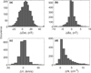 |
Fig. 4 The deviation of hourly averaged final data (OMNI) from hourly averaged real-time data for disturbed periods Dst < − 50 nT over the period of July 2011–December 2016. (a) Dst index (nT). (b) Southward IMF Bz (nT). (c) Solar wind velocity V (km/s). (d) Solar wind density N (cm−3). |
The summary of reasons for the decrease of forecast quality using real-time input.
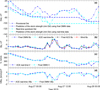 |
Fig. 5 The geomagnetic storm on 26–28 August 2015. (a) Provisional Dst (dashed blue); predictions of the peak Dstp using final OMNI input (solid blue); real-time quicklook Dst (dashed cyan); predictions of real-time Dstp using real-time input (solid cyan). (b) Final OMNI IMF Bz (blue); ACE real-time IMF Bz (cyan); Final ACE IMF Bz (level 2, black); Wind Bz (not shifted original data, red). (c) Final OMNI solar wind speed V (cyan); ACE real-time solar wind speed V (blue). (d) Final OMNI parameter VBs (cyan); ACE real-time parameter VBs (blue). |
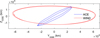 |
Fig. 8 Position of ACE (blue) and Wind (red) in 2011. |
5 Conclusion
In this study, we review performance of the geomagnetic storm forecasting service StormFocus at SpaceWeather.Ru during more than 5 years of operation from July 2011 to December 2016. The service provides the warnings on the expected geomagnetic storm magnitude for the next several hours on an hourly basis. The maximum of the solar cycle 24 was weak, so the most of statistics were rather moderate storms. We verify the quality of forecasts and selection criteria, as well as the reliability of online input data to predict the geomagnetic storm strength in comparison with the final values available in archives. We also analyze the sources of prediction errors and identified the errors that cannot be removed in real-time and those that can be fixed by improving the prediction algorithm.
StormFocus service on the basis of ACE real-time and quicklook Dst data issued the successful forecast of peak Dstp (within 25% of the actual storm magnitude) for 129 out of 153 geomagnetic storms with the detection probability of 0.87. The algorithm rerun on final OMNI data provided the successful forecast for 148 storms with the detection probability of 0.97. An important measure of the practical usefulness of the real-time forecast is the prediction of the actual final Dstp using the real-time input. It was successful for 130 storms with the detection probability of 0.9. Therefore we confirmed the general reliability of the StormFocus service to provide the advance warnings of geomagnetic storm strength over the period 2011–2016.
Several error sources require special attention. First of all, forecast in real-time operation is somewhat less reliable, than on the final archived data due to errors or imperfections of the real-time input, both solar wind, IMF and Dst. Such reasons accounted for more than a half of all forecast errors. In particular such reasons most likely explain a strong increase of a number of later overestimates (after successful forecast was given) from ∼10% to 24%, when the real-time data are compared with the final index.
Real-time errors are often overlooked during performance analysis, since they are nominally beyond control during an algorithm design. One can advise to verify the forecast quality additionally on the real-time data streams if available. Statistics on expected differences between real-time and final data would be also very helpful. Alternatively one may use the forecast models with the probabilistic output (providing the range of possible values with some degree of certainty), however such models require much larger data amounts for training.
The second substantial error was related with the generation of the “sudden” storm warning, based on a sharp increase of VBs. In real-time about a half of the “sudden” storms were missed and several false warnings were generated. The primary reason was again related with the differences between real-time and final data. To remediate such errors we additionally introduced in the algorithm a condition, canceling the warning in a case it was caused by a single-point peak in VBs. However, it should be noted, that the sudden storm variant of the forecast was designed to warn on very strong storms (as it was during period 1995–2010, used for the design). Stronger storms are usually related with more stable solar wind and IMF input and develop faster, thus extrapolations in our forecast are more reliable. During the test period the storms were much weaker on average, practically all “sudden” storms were weaker (less negative) than −150 nT. For such events “sudden” storm warnings are expected to be less reliable.
In conclusion, the geomagnetic storm forecasting service StormFocus that provides the warnings of future geomagnetic storm magnitude proved to be quite successful after more than five years of online operation and can be recommended for applications. A few of the most registered forecast failures were caused by the errors in the real-time input data (relative to final data, appearing later). This source of errors needs special attention during the forecast algorithm design.
Acknowledgements
The authors are grateful to the National Space Science Data Center for the OMNI 2 database, to the National Oceanic and Atmospheric Administration (NOAA) for ACE real-time solar wind (RTSW) data, to the WDC for Geomagnetism (Kyoto) for the Dst index data. We thank the referee for valuable comments on this study. The work was supported by Russian Science Foundation, N16-12-10062. The editor thanks two anonymous referees for their assistance in evaluating this paper.
Appendix A The prediction of storm strength
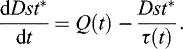
The prediction technique of the peak Dstp during geomagnetic storms is based on the differential equation of the Dst index evolution introduced by Burton et al. (1975) as a functional relation between solar wind and Dst.
 (A.1)
Here Q (mV/m) is the solar wind input function. We use the model variant by O'Brien and McPherron (2000b), where the parameter Q is linearly connected with the driving parameter VBs.
(A.1)
Here Q (mV/m) is the solar wind input function. We use the model variant by O'Brien and McPherron (2000b), where the parameter Q is linearly connected with the driving parameter VBs.
 (A.2)
(A.2)
 (A.3)
(A.3)
 (A.4)Here V (km/s) is solar wind plasma speed, Bs (nT) is southward component of IMF in GSM, Pdyn (nPa) is solar wind dynamic pressure, and τ (hours) is decay time constant, associated with the loss processes in the inner magnetosphere. Dst* is the pressure corrected Dst index, from which the effects of the magnetopause currents have been removed. However, we neglect the difference between Dst and Dst*, and do not compute this pressure correction, because generally it is rather small, and often real-time solar wind density is quite different from the calibrated data, appearing later in the archives.
To predict future strength of a storm we use the solution of the differential Equation (A.1) with an initial condition (solar wind, IMF and quick-look Dst) taken at some “zero” moment and assuming stationary solar wind input, equal to that at the initial point (hereafter Q0, τ0).
 (A.5)
This solution is the monotonously decreasing function of time, and when t→ ∞, it approaches the steady-state value.
(A.5)
This solution is the monotonously decreasing function of time, and when t→ ∞, it approaches the steady-state value.
We compute two variants of the forecast Dst. The storm saturation level reached at the steady-state solution is used as a prediction of the lower limit of peak Dstp.
 (A.6)
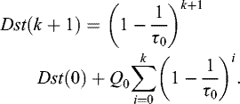
To predict the upper limit we select the intermediate point on the saturation trajectory determined by the solution of the discrete variant of Equation (A.1) given by
(A.6)
To predict the upper limit we select the intermediate point on the saturation trajectory determined by the solution of the discrete variant of Equation (A.1) given by
 (A.7)The solution of this equation k hours ahead for constant Q and τ is
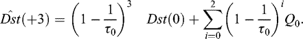
 (A.8)As the upper limit we use the three-hours-ahead extrapolation, which was justified by the statistics.
 (A.9)
(A.9) is computed routinely every hour, and to avoid its excessive variability the final prediction
  is kept at the minimum of all
  obtained after the last “storm end” flag. The “storm end” is signaled and
  returns to the current
  , when IMF Bz ≥ 1 nT during 3 hours or IMF Bz ≥ − 1.8 nT during 11 hours.
The prediction of both upper and lower limits,  and Dst(∞), of the peak Dstp is proved to be useful only for a group of larger “sudden” storms, associated with a sufficiently sharp increase of VBs. All other storms are then called gradual.
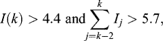
We introduced the following criteria for the sharp increase of VBs: I(k) = VBs(k) − VBs(k − 1):
 (A.10)
 (A.11)
The thresholds in (A.10), (A.11) are given in mV/m. Condition (A.10) checks for the sharp increase of VBs during last three hours and the last hour in particular. Condition (A.11) requires that VBs is sufficient to cause a strong enough storm. Numerical coefficients in (A.10), (A.11) were selected empirically on historical data to perform the best possible forecast.
(A.11)
The thresholds in (A.10), (A.11) are given in mV/m. Condition (A.10) checks for the sharp increase of VBs during last three hours and the last hour in particular. Condition (A.11) requires that VBs is sufficient to cause a strong enough storm. Numerical coefficients in (A.10), (A.11) were selected empirically on historical data to perform the best possible forecast.
We issue a forecast of future “sudden” storm strength at a specific moment of VBs jump when both criteria (A.10), (A.11) are fulfilled. We expect a stable prolonged storm-grade solar wind input and define both a lower limit Dst(∞) and an upper limit  , so that the real peak value is expected to be between
  . For weaker storms with VBs < 10.9 mV/m, when Dst(∞) < − 150 nT, we use Dst(∞) =0.85Q0 ⋅ τ0, since such storms require too long time to approach their saturation value. This two-level forecast works best for the strongest storms, with shorter saturation times (proportional to τ in Burton equation).
Gradually developing storms (for which “sudden” criterion is not fulfilled) usually has longer saturation times, while variability of the input is larger, thus such events are rarely reaching expected saturation level. For such events the prediction of peak Dstp is performed on the basis of three-hour forecast  only. The storm alert is issued when the forecast of peak Dstp reaches the threshold of −50 nT.
Reviewing the performance of the algorithm during more than 5 years of operation, we partially modified the criteria to detect “sudden” storms, associated with a sharp increase of VBs. Single-point outliers in real-time VBs are actually observed more often than in final data. To minimize the risk of false “sudden” storm warnings, the jump criteria (A.10), (A.11) are now augmented with the rule, cancelling the “sudden” storm warning if it was generated due to a single-point outlier in Q: The lower limit is removed from the forecast, when VBs ≤ 3 at step k, VBs < 5.5 over two hours at steps k − 2 and k − 3, and the conditions (A.10), (A.11) were fulfilled at previous step k − 1. Over the period of July 2011–December 2016 there were 5 such cases.
References
- Akasofu SI. 1981. Prediction of development of geomagnetic storms using the solar wind-magnetosphere energy coupling function epsilon. Planet Space Sci 29: 1151–1158. [CrossRef] [Google Scholar]
- Amata E, Pallocchia G, Consolini G, Marcucci MF, Bertello I. 2008. Comparison between three algorithms for Dst predictions over the 2003–2005 period. J Atmos Solar-Terr Phys 70: 496–502. [CrossRef] [Google Scholar]
- Andriyas T, Andriyas S. 2015. Relevance vector machines as a tool for forecasting geomagnetic storms during years 1996–2007. J Atmos Solar-Terr Phys 125: 10–20. [CrossRef] [Google Scholar]
- Bala R, Reiff P. 2012. Improvements in short-term forecasting of geomagnetic activity. Space Weather 10: S06001. [CrossRef] [Google Scholar]
- Boynton RJ, Balikhin MA, Billings SA, Amariutei OA. 2013. Application of nonlinear autoregressive moving average exogenous input models to geospace: advances in understanding and space weather forecasts. Ann Geophys 31: 1579–1589. [CrossRef] [Google Scholar]
- Boynton RJ, Balikhin MA, Billings SA, Sharma AS, Amariutei OA. 2011. Data derived NARMAX Dst model. Ann Geophys 29: 965–971. [CrossRef] [Google Scholar]
- Burton RK, McPherron RL, Russell CT. 1975. An empirical relationship between interplanetary conditions and Dst. J Geophys Res 80: 4204–4214. [Google Scholar]
- Caswell JM. 2014. A nonlinear autoregressive approach to statistical prediction of disturbance storm time geomagnetic fluctuations using solar data. J Signal Inf Process 5: 42–53. [Google Scholar]
- Chen J, Slinker SP, Triandaf I. 2012. Bayesian prediction of geomagnetic storms: wind data, 1996–2010. Space Weather 10: S04005. [CrossRef] [Google Scholar]
- Echer E, Gonzalez WD, Tsurutani BT, Gonzalez ALC. 2008. Interplanetary conditions causing intense geomagnetic storms (Dst ≤ − 100 nT) during solar cycle 23. J Geophys Res 113: A05221. [Google Scholar]
- Echer E, Tsurutani BT, Gonzalez WD. 2013. Interplanetary origins of moderate (100 nT < Dst ≤ − 50 nT) geomagnetic storms during solar cycle 23 (1996Â-2008). J Geophys Res: Space Phys 118: 385–392. [CrossRef] [Google Scholar]
- Gonzalez WD, Echer E. 2005. A study on the peak Dst and peak negative Bz relationship during intense geomagnetic storms. Geophys Res Lett 32: L18103. [CrossRef] [Google Scholar]
- Gonzalez WD, Joselyn JA, Kamide Y, Kroehl HW, Rostoker G, Tsurutani BT, Vasyliunas VM. 1994. What is a geomagnetic storm? J Geophys Res 99: 5771–5792. [NASA ADS] [CrossRef] [Google Scholar]
- Ji EY, Moon YJ, Gopalswamy N, Lee DH. 2012. Comparison of Dst forecast models for intense geomagnetic storms. J Geophys Res (Space Phys) 117: A03209. [Google Scholar]
- Kane RP, Echer E. 2007. Phase shift (time) between storm-time maximum negative excursions of geomagnetic disturbance index Dst and interplanetary Bz. J Atmos Sol Terr Phys 69: 1009–1020. [CrossRef] [Google Scholar]
- Katus RM, Liemohn MW, Ionides EL, Ilie R, Welling D, Sarno-Smith LK. 2015. Statistical analysis of the geomagnetic response to different solar wind drivers and the dependence on storm intensity. J Geophys Res: Space Phys 120: 310–327. [CrossRef] [Google Scholar]
- Lundstedt H, Gleisner H, Wintoft P. 2002. Operational forecasts of the geomagnetic Dst index. Geophys Res Lett 29: 2181. [Google Scholar]
- Mansilla GA. 2008. Solar wind and IMF parameters associated with geomagnetic storms with Dst ≤−50 nT. Phys Scr 78: 045902. [CrossRef] [Google Scholar]
- Nikolaeva NS, Yermolaev YI, Lodkina IG. 2014. Dependence of geomagnetic activity during magnetic storms on the solar wind parameters for different types of streams: 4. Simulation for magnetic clouds. Geomagn Aeron 54: 152–161. [CrossRef] [Google Scholar]
- O'Brien TP, McPherron RL. 2000a. An empirical phase space analysis of ring current dynamics: solar wind control of injection and decay. J Geophys Res 105: 7707–7720. [CrossRef] [Google Scholar]
- O'Brien TP, McPherron RL. 2000b. Forecasting the ring current index Dst in real time. J Atmos Sol Terr Phys 62: 1295–1299. [Google Scholar]
- Pallocchia G, Amata E, Consolini G, Marcucci MF, Bertello I. 2006. Geomagnetic Dst index forecast based on IMF data only. Ann Geophys 24: 989–999. [CrossRef] [Google Scholar]
- Petrukovich AA, Klimov SI. 2000. The use of solar wind measurements for the analysis and prediction of geomagnetic activity. Cosm Res 38: 433. [Google Scholar]
- Petrukovich AA, Klimov SI, Lazarus A, Lepping RP. 2001. Comparison of the solar wind energy input to the magnetosphere measured by Wind and Interball-1. J Atmos Solar-Terr Phys 63: 1643–1647. [CrossRef] [Google Scholar]
- Podladchikova TV, Petrukovich AA. 2012. Extended geomagnetic storm forecast ahead of available solar wind measurements. Space Weather 10: S07001. [CrossRef] [Google Scholar]
- Rastätter L, Kuznetsova MM, Glocer A, Welling D, Meng X et al. 2013. Geospace environment modeling 2008Â-2009 challenge: Dst index. Space Weather 11: 187–205. [CrossRef] [Google Scholar]
- Rathore BS, Dinesh CG, Parashar KK. 2014. A nonlinear autoregressive approach to statistical prediction of disturbance storm time geomagnetic fluctuations using solar data. J Signal Inf Process 5: 42–53. [Google Scholar]
- Revallo M, Valach F, Hejda P, Bochníček J. 2014. A neural network Dst index model driven by input time histories of the solar wind-magnetosphere interaction. J Atmos Sol-Terr Phys 110: 9–14. [Google Scholar]
- Sharifie J, Lucas C, Araabi B. 2006. Locally linear neurofuzzy modeling and prediction of geomagnetic disturbances based on solar wind conditions. Space Weather 4: S06003. [CrossRef] [Google Scholar]
- Siscoe G, McPherron RL, Liemohn MW, Ridley AJ, Lu G. 2005. Reconciling prediction algorithms for Dst. J Geophys Res 110: A02215. [Google Scholar]
- Temerin M, Li X. 2002. A new model for the prediction of Dst on the basis of the solar wind. J Geophys Res 107: 1472. [CrossRef] [Google Scholar]
- Temerin M, Li X. 2006. Dst model for 1995–2002. J Geophys Res 111: A04221. [CrossRef] [Google Scholar]
- Valdivia JA, Sharma AS, Papadopoulos K. 1996. Prediction of magnetic storms by nonlinear models. Geophys Res Lett 23: 2899–2902. [CrossRef] [Google Scholar]
- Vassiliadis D, Klimas A, Baker D. 1999. Models of Dst geomagnetic activity and of its coupling to solar wind parameters. Phys Chem Earth 24: 107–112. [Google Scholar]
- Wei HL, Billings SA, Balikhin M. 2004. Prediction of the Dst index using multiresolution wavelet models. J Geophys Res 109: A07212. [Google Scholar]
- Wing S, Johnson JR, Jen J, Meng CI, Sibeck DG, Bechtold K, Freeman J, Costello K, Balikhin M, Takahashi K. 2005. Kp forecast models. J Geophys Res (Space Phys) 110: A04203. [Google Scholar]
- Wu JG, Lundstedt H. 1997. Geomagnetic storm predictions from solar wind data with the use of dynamic neural networks. J Geophys Res 102: 14255–14268. [Google Scholar]
- Yermolaev YI, Nikolaeva NS, Lodkina IG, Yermolaev MY. 2010. Specific interplanetary conditions for CIR-, Sheath-, and ICME-induced geomagnetic storms obtained by double superposed epoch analysis. Ann Geophys 28: 2177–2186. [CrossRef] [Google Scholar]
- Yermolaev YI, Yermolaev MY. 2002. Statistical relationships between solar, interplanetary, and geomagnetospheric disturbances, 1976–2000. Cosm Res 40: 1–14. [NASA ADS] [CrossRef] [Google Scholar]
- Yermolaev YI, Yermolaev MY, Zastenker GN, Zelenyi LM, Petrukovich AA, Sauvaud JA. 2005. Statistical studies of geomagnetic storm dependencies on solar and interplanetary events: a review. Planet Space Sci 53: 189–186. [CrossRef] [Google Scholar]
- Zhu D, Billings SA, Balikhin M, Wing S, Coca D. 2006. Data derived continuous time model for the Dst dynamics. Geophys Res Lett 33: L04101. [Google Scholar]
- Zhu D, Billings SA, Balikhin MA, Wing S, Alleyne H. 2007. Multi-input data derived Dst model. Geophys Res Lett 112: A06205. [Google Scholar]
Cite this article as: Podladchikova T, Petrukovich A, Yermolaev Y. 2018. Geomagnetic storm forecasting service StormFocus: 5 years online. J. Space Weather Space Clim. 8: A22
All Tables
Forecast statistics for: “RR” − real-time quicklook Dstp prediction using real-time input; “FF” − final Dstp prediction using final input; “RF” − final Dstp prediction using real-time input.
The probability of detection (POD) and the ratio of overestimated forecasts (ROF) of the earliest and maximal forecasts for the three types of the forecast run: “RR” − real-time quicklook Dstp prediction using real-time input; “FF” − final Dstp prediction using final input; “RF” − final Dstp prediction using real-time input.
The summary of reasons for the decrease of forecast quality using real-time input.
All Figures
|
Fig. 1 Layout of the StormFocus forecast web page for the geomagnetic storm on 6 August 2011. |
| In the text | |
|
Fig. 2 Forecast statistics for “sudden” geomagnetic storms. (a) Storm predictions using real-time data input. (1) final Dstp; (2) the earliest prediction of both upper and lower limits of Dstp within 25% of actual storm magnitude; (3) the earliest prediction of Dstp with 3-hour forecast (not “sudden” in real-time); (4) and (5) the predictions of Dstp, which were out of 25% range from actual Dstp. (b) Storm predictions using final data input. (6) final Dstp; (7) the earliest prediction of both upper and lower limits of Dstp within 25% of actual storm magnitude; (8) the predictions of Dstp, which were out of 25% range from actual storm magnitude. (c) The advance warning time (in hours) of the Dstp forecast using real-time input. |
| In the text | |
|
Fig. 3 Forecast statistics for “gradual” geomagnetic storms. (a) Storm predictions using real-time data input. (1) final Dstp; (2) the earliest prediction of Dstp within 25% of actual storm magnitude; (3) the predictions of Dstp, which were out of 25% range; (4) maximal predictions of Dstp obtained during the storm development; (5) maximal predictions out of 25% range. (b) Storm predictions using final data input. (6) final Dstp; (7) the earliest prediction of Dstp within 25%; (8) the predictions of Dstp, which were out of 25% range; (9) maximal predictions of Dstp obtained during the storm development; (10) maximal predictions out of 25% range. (c) The advance warning time (in hours) of the Dstp forecast using real-time input. |
| In the text | |
|
Fig. 4 The deviation of hourly averaged final data (OMNI) from hourly averaged real-time data for disturbed periods Dst < − 50 nT over the period of July 2011–December 2016. (a) Dst index (nT). (b) Southward IMF Bz (nT). (c) Solar wind velocity V (km/s). (d) Solar wind density N (cm−3). |
| In the text | |
|
Fig. 5 The geomagnetic storm on 26–28 August 2015. (a) Provisional Dst (dashed blue); predictions of the peak Dstp using final OMNI input (solid blue); real-time quicklook Dst (dashed cyan); predictions of real-time Dstp using real-time input (solid cyan). (b) Final OMNI IMF Bz (blue); ACE real-time IMF Bz (cyan); Final ACE IMF Bz (level 2, black); Wind Bz (not shifted original data, red). (c) Final OMNI solar wind speed V (cyan); ACE real-time solar wind speed V (blue). (d) Final OMNI parameter VBs (cyan); ACE real-time parameter VBs (blue). |
| In the text | |
 |
Fig. 6 The same as Figure 5 except for the geomagnetic storm on 1–2 November 2011. |
| In the text | |
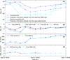 |
Fig. 7 The same as Figure 5 except for the geomagnetic storm on 11 September 2011. |
| In the text | |
|
Fig. 8 Position of ACE (blue) and Wind (red) in 2011. |
| In the text | |
Current usage metrics show cumulative count of Article Views (full-text article views including HTML views, PDF and ePub downloads, according to the available data) and Abstracts Views on Vision4Press platform.
Data correspond to usage on the plateform after 2015. The current usage metrics is available 48-96 hours after online publication and is updated daily on week days.
Initial download of the metrics may take a while.