| Issue |
J. Space Weather Space Clim.
Volume 8, 2018
|
|
|---|---|---|
| Article Number | A47 | |
| Number of page(s) | 10 | |
| DOI | https://doi.org/10.1051/swsc/2018033 | |
| Published online | 23 October 2018 | |
Research Article
Forecasting Solar Energetic Particle (SEP) events with Flare X-ray peak ratios
1
Space Vehicles Directorate, AFRL/RVBXD, Bldg 570, 3550 Aberdeen Dr. SE, Kirtland AFB, NM 87110, USA
2
Atmospheric Environmental Research, 2201 Buena Vista Drive SE, Suite 407, Albuquerque, NM 87106, USA
* Corresponding author: This email address is being protected from spambots. You need JavaScript enabled to view it.
Received:
2
March
2018
Accepted:
6
September
2018
Abstract
Solar flare X-ray peak fluxes and fluences in the 0.1–0.8 nm band are often used in models to forecast solar energetic particle (SEP) events. Garcia (2004) [Forecasting methods for occurrence and magnitude of proton storms with solar soft X rays, Space Weather, 2, S02002, 2004] used ratios of the 0.05–0.4 and 0.1–0.8 nm bands of the X-ray instrument on the GOES spacecraft to plot inferred peak flare temperatures versus peak 0.1–0.8 nm fluxes for flares from 1988 to 2002. Flares associated with E > 10 MeV SEP events of >10 proton flux units (pfu) had statistically lower peak temperatures than those without SEP events and therefore offered a possible empirical forecasting tool for SEP events. We review the soft and hard X-ray flare spectral variations as SEP event forecast tools and repeat Garcia’s work for the period 1998–2016, comparing both the peak ratios and the ratios of the preceding 0.05–0.4 nm peak fluxes to the later 0.1–0.8 nm peak fluxes of flares >M3 to the occurrence of associated SEP events. We divide the events into eastern and western hemisphere sources and compare both small (1.2–10 pfu) and large (≥300 pfu) SEP events with those of >10 pfu. In the western hemisphere X-ray peak ratios are statistically lower for >10 pfu SEP events than for non-SEP events and are even lower for the large (>300 pfu) events. The small SEP events, however, are not distinguished from the non-SEP events. We discuss the possible connections between the flare X-ray peak ratios and associated coronal mass ejections that are presumed to be the sources of the SEPs.
Key words: energetic particles / forecasting / space radiation environment
© S.W. Kahler & A.G. Ling, Published by EDP Sciences 2018
 This is an Open Access article distributed under the terms of the Creative Commons Attribution License (http://creativecommons.org/licenses/by/4.0), which permits unrestricted use, distribution, and reproduction in any medium, provided the original work is properly cited.
1 Introduction
The deleterious effects of energetic (E > 10 MeV) particle radiation on humans in space (Schwadron et al., 2017) and on space systems technology (Tribble, 2010; Crosby et al., 2015) have motivated efforts to forecast Solar Energetic Particle (SEP) events based on observations of solar eruptive events. Large NOAA (≥10 proton flux units (pfu = 1 proton/(cm2 s sr)), at E > 10 MeV) SEP events are produced by acceleration in shocks driven by broad (>60°) coronal mass ejections (CMEs; e.g., Reames, 2013) which are usually accompanied by large (>M1) flares as measured by the full-Sun X-Ray Sensors (XRS) on the GOES spacecraft. Measured speeds and widths of CMEs are desirable for SEP event forecasting, but X-ray flare events precede the associated CMEs and have shorter timescales (St. Cyr et al., 2017), making X-ray flares the standard tool for rapid forecasting of SEP events.
The XRS 0.1–0.8 nm band flux profiles are measured every 3 s and available in real time with 1 minute averages (Garcia, 1994b). The 0.1–0.8 nm flare peak fluxes or time-integrated fluences are used by the Air Force Research Laboratory Proton Prediction System (PPS; Smart & Shea, 1992; Kahler et al., 2007, 2017); PROTONS (Balch, 2008); the IZMIRAN prognostic practice (Belov, 2009), the Empirical model for Solar Proton Events Real Time Alert (ESPERTA) (Alberti et al., 2017); Solar Particle Radiation SWx (SPARX) (Marsh et al., 2015); and Forecasting Solar Particle Events and Flares (FORSPEF) (Papaioannou et al., 2015; Anastasiadis et al., 2017). These models differ in terms of their other required inputs, such as flare solar locations and accompanying radio bursts, and of their outputs, such as SEP event occurrences, peak intensities and timings.
1.1 Hard X-ray bursts and SEP events
Garcia (1994a) reviewed early work to associate properties of hard (E > 30 keV) and soft X-ray flares with subsequent SEP events. In the first case, good associations were found between gradual (durations >10 min) hard X-ray (GHX) flares, which were a small minority (<3%) of all hard X-ray flares, and SEP events. A key characteristic of GHX flares observed with the HXRBS instrument on the Solar Maximum Mission (SMM) spacecraft (Bai, 1986) was the tendency of the spectrum to harden through the event (described as soft-hard-harder or SHH), in contrast to the soft-hard-soft SHS spectral behavior of impulsive hard X-ray flares. Kiplinger (1995) did two different comparisons between NOAA SEP events and hard X-ray bursts observed with the HXRBS/SMM instrument, the second of which used only one third of the candidate burst population. Combining results of the first comparison and the weighted results of the second, he got a projected result that the SHH flare criterion would correctly forecast a NOAA SEP event in 22 of 23 cases and that forecasts of no SEP event, based on an absence of the SHH criterion, would be correct in 700 of 708 cases.
Garcia (2004b) used a slightly different criterion requiring a hard spectral index of γ < 4 for flares observed with a hard X-ray spectrometer on the Multispectral Thermal Imaging spacecraft. That criterion forecast 14 of 16 associated SEP events, with two missed events and three false forecasts. The SHH criterion was used by Grayson et al. (2009) to examine 37 hard X-ray bursts (HXBs) observed with the RHESSI spacecraft and their SEP event associations, and they found that 12 of 18 flares with the SHH criterion correctly forecast SEP events with peak intensities >0.1 pfu and that none of the 19 events without the SHH criterion was followed by a SEP event.
These SHH HXB and SEP event studies were reviewed in detail by Kahler (2012), who discussed several limiting factors of the analyses. First, reverse comparisons, in which one starts with observed SEP events and then asks whether they would have been forecast with GHX flares, were not included. In addition, flares were generally limited to those with well connected solar longitudes. The numbers of SEP events missed with the SHH criterion were lower when the authors included SEP events of any size versus only the NOAA SEP events, and good contingency table statistics were sometimes heavily weighted by small HXBs and no observed SEP events. Finally, the time-interval and X-ray energy range criteria for defining the SHH spectral behavior are not well defined, and a sequence of smaller non-SHH XRBs may appear as an SHH XRB. There is a strong connection between GHXBs and fast CMEs, the drivers of SEP-accelerating shocks, which accounts for the utility of using GXBs as SEP event forecast tools (Kahler, 2012).
1.2 Soft X-ray flare temperatures and SEP events
The GOES XRS measures two X-ray wavebands with ion chamber detectors, the nominal 0.05–0.4 nm and the 0.1–0.8 nm bands (Garcia, 1994b). The ratio of the 0.05–0.4 nm to the 0.1–0.8 nm fluxes in solar flare events yields the flare plasma temperature and emission measure, assuming a single temperature source. The conversion from detector flux ratios to temperatures depends on the assumed model of thermal emission, and the earlier assumed models (Garcia, 1994b) have evolved to the currently used version (White et al., 2005), which accounts for coronal abundances. For current SEP forecasting models, only the 0.1–0.8 nm band has been utilized, with two exceptions to our knowledge. Ji et al. (2014) used three GOES X-ray flare parameters, one of which was the flare emission measure, to construct a model to forecast the peak E > 10 MeV SEP-event intensities. Although they give no information on the source of the emission measure, a time-varying quantity, we assume it is derived from the ratio of the GOES 0.05–0.4 nm and 0.1–0.8 nm bands. Winter and Balasubramaniam (2015) plotted the maximum ratio of the 0.05–0.4 nm to 0.1–0.8 nm flare fluxes against their 0.1–0.8 nm backgrounds to achieve a separation among ~50 000 B, C, M, and X-class flares (their Fig. 4). Considering the extra flare information obtained from both XRS bands rather than only the 0.1–0.8 nm band, it is prudent to consider how the combination of the two bands can help to improve the SEP forecasting techniques. Here we revisit the earlier work on exactly that topic by Garcia (1994a, 2004a).
2 Data analysis
Garcia did two similar plots of maximum flare X-ray temperatures versus logs of 0.1–0.8 nm peak flux, the first over the period 1977–1991 (Garcia, 1994a), and the second from 1988 to 2002 (Garcia, 2004a). Figure 1 is a reproduction of the Garcia (2004a) plot of 1460 > M1 flares, showing with diamonds flares associated with the 87 NOAA SEP events. Each distribution in the figure is fitted with a quadratic polynomial, and the SEP flares clearly have statistically cooler temperatures.
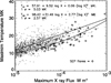 |
Fig. 1. Maximum X-ray flare temperatures versus maximum 0.1–0.8 nm flare fluxes for the period 1988–2002. NOAA SEP events are indicated with diamonds (from Garcia, 2004a). |
We have selected all GOES flares >M3 with known flare locations from 1998 to 2016 for our analysis. The numbers of all the 433 solar flares in eastern and western longitude ranges are shown in Table 1. They were first divided into three groups with the following SEP event associations: (1) a no-associated (No-SEP) event; (2) a 1.2–10 pfu (small) SEP event; and (3) a NOAA > 10-pfu SEP event. A high-intensity (≥300 pfu) subset of the NOAA group was also selected for further study. All the SEP events were drawn from a comprehensive table of E > 10 MeV proton events over the same time period that we have compiled and are being publishing separately (Kahler & Ling, 2018) for another study.
Numbers of SEP events by solar hemisphere.
We calculated the 0.05–0.4 nm and 0.1–0.8 nm X-ray flare fluxes by subtracting from the total fluxes, obtained from the satdat.ngdc.noaa.gov website, their estimated backgrounds of the previous several hours. In addition, for the X-ray flares we used two ratios of (0.05–0.4 nm)/(0.1–0.8 nm) fluxes: (1) the peaks of the flux ratios, occurring at the peaks of the 0.05–0.4 nm fluxes and corresponding to the maximum temperatures (Garcia, 2004a), and (2) the ratios of the two peak fluxes, in which the 0.1–0.8 nm peak always follows the 0.05–0.4 nm peak by ≈3–10 min (Winter & Balasubramaniam, 2015). We prefer to use the ratio of directly available X-ray fluxes, rather than a temperature conversion, as was done by Garcia (2004a, Fig. 1). The goal of comparing the two peak values was to see whether ratio plots of (2) differentiated the SEP and non-SEP events better than the ratio plots of (1). Figure 2 shows the comparison of plots with the two different ratios and quadratic polynomial fits for each of the three SEP event populations. In both plots we find, in accord with Garcia (2004a), that the NOAA SEP events have generally cooler associated X-ray flare temperatures than the No-SEP events and furthermore that the small SEP events are only slightly separated from the No-SEP events. With no obvious difference between the peak-of-ratio and ratio-of-peak plots in the separations of populations, we continue the analysis using only the peak-of-ratios plots.
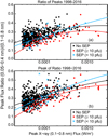 |
Fig. 2. (a) Ratios of the 0.05–0.4 nm and 0.1–0.8 nm peak fluxes versus peak 0.1–0.8 nm flare fluxes for No-SEP, NOAA, and small SEP events. (b) Peaks of the flux ratios, corresponding to maximum temperatures, versus peak 0.1–0.8 nm flare fluxes for the same SEP event classes. The peaks of flux ratios in this plot are adopted for subsequent analysis. Quadratic fits to each group are shown. |
In Figure 3 we divide the events into eastern (top) and western (bottom) hemisphere longitudes to look for separations between the No-SEP flares and the small (blue crosses) and NOAA (red dots) SEP events. We do a quantitative population comparison by calculating t-test scores on bins of the plots, as did Garcia (1994a) for an earlier version of his plot shown in Figure 1. The t-test gives the probability P that two populations in a given bin are drawn from the same source population. While Garcia (1994a) examined bins defined by peak X-ray flux ranges, we use bins defined by peak flux ratios because the No-SEP and SEP populations show more separation along the log peak-flux axis than along the peak flux-ratio axis. We list the t-test scores t and P in Table 2 for each of the comparisons. The last column of Table 2 gives the compared populations and relevant figure numbers. We limit all comparisons to three bins of nearly equal numbers of total events in each bin in each hemisphere (i.e., 247/3 and 261/3 events in the eastern and western hemispheres, respectively). The resulting bin boundaries are nearly the same for both hemispheres and are given in column 2. The P values are generally very small, <10−2, but their relative values tell us how well different SEP populations are separated from the larger No-SEP flares.
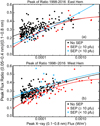 |
Fig. 3. (a) Peak-flux ratios versus 0.1–0.8 nm peak fluxes for the No-SEP, small (blue crosses), and NOAA events (red dots) in the eastern hemisphere. Quadratic polynomial fits to each distribution are shown. (b) Same for the western hemisphere events. |
T-test distribution differences between groups of events.
The small (<10 pfu) SEP events are not well separated from the No-SEP flares in Figure 3. P > 0.1 for two of the three corresponding bins in both the eastern and western hemispheres. The two remaining bins with small (<3 × 10⁻⁴) P values are characterized by only a few small events. However, in the eastern hemisphere there is a cluster of small events in the lower left part of the plot. A t-test analysis based on bins of log peak X-ray flux does show a modest P < 0.05 for the two flux bins <8.34 × 10⁻⁵ W m−2, but that separation is not strong. The NOAA events are well separated from the No-SEP flares in all bins of both hemispheres.
We are also interested in whether or how well the peak-flux ratio can discriminate between the largest (≥300 pfu) NOAA SEP events and the remaining population of <300 pfu NOAA events. Figure 4 compares the eastern and western hemispheres for which the small SEP events are merged together with the No-SEP flares and then compared to both kinds of NOAA events (crosses). There are only five ≥300 pfu events in the eastern hemisphere, but they are consistent with no difference between the two populations of NOAA events.
 |
Fig. 4. (a) The peak-flux ratios versus 0.1–0.8 nm peak fluxes for the combined No-SEP and small (<10 pfu) SEP events, large (≥300 pfu) NOAA events (red crosses), and the remaining smaller NOAA events (blue crosses) for eastern hemisphere events. Quadratic polynomial fits are shown as lines in matching colors. (b) The same for western hemisphere events. |
In the west, however, Table 2 shows that P values of the ≥300 pfu NOAA events are more than three orders of magnitude lower than those of the remaining smaller NOAA events in all three peak flux-ratio bins. We have divided the western hemisphere into three longitude regions and examined peak-ratio plots of each region to look for any obvious further longitude dependences within the hemisphere, but with the limited numbers of SEP events shown in Table 1 we found no clear dependences. Finally, in Figure 5a and b we show the flux ratios in the two hemispheres plotted for only the basic NOAA SEP events. The corresponding P values of Table 2 for each peak flux-ratio range are smaller for the western hemisphere than for the eastern hemisphere, reflecting the better separation of NOAA events in the western hemisphere.
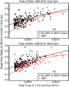 |
Fig. 5. (a) Peak flux ratios versus 0.1–0.8 nm peak fluxes for NOAA SEP events in the eastern hemisphere. Solid lines are polynomial quadratic best fits. (b) Same for the western hemisphere. |
For his temperature plots, equivalent to the peak flux-ratio plots in this work, Garcia (1994a, 2004a) produced a set of SEP event probability contours based on a logistic regression analysis. With the same purpose of exhibiting a practical forecast application, we have subjected the western hemisphere plot of Figure 5b to two selected machine learning classifier techniques, which use the observed data points to generate plots showing which of the event classes is most likely at any given point. In our case, we have the simple case of only two classes of No-SEP or NOAA SEP events.
Using the neural-net and nearest-neighbor algorithms from the Python machine-learning library [scikit-learn] (Pedregosa et al., 2011), we show the results in Figure 6. The neural-net algorithm we used is the multi-layer perceptron, described by Gardner & Dorling (1998). We used default weights and inputs to run the module. The nearest-neighbor classification of Figure 6b is computed from a simple majority vote of the k nearest neighbors of each point. A query point is assigned the data class which has the most representatives within the nearest neighbors of the point. The optimal choice of the value k is highly data-dependent. A larger k suppresses the effects of noise, but makes the classification boundaries less distinct. We used k = 13 and uniform weighting. There are additional parameters that one can give the classifier, but we used the default values for all of them. The results are compared in Figure 6, where we find that the nearest neighbor algorithm gives more ragged boundaries (Fig. 6b) than does the neural net of Figure 6a, and is therefore probably more difficult to implement for a forecasting tool. Because we have only 18 NOAA events out of 229 flares in the eastern hemisphere (Fig. 5a), both algorithms classify all or nearly all of the X-ray peak-ratio versus peak-flux space in that hemisphere as No-SEP regions; those plots are not shown.
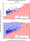 |
Fig. 6. (a) The western hemisphere peak-flux ratios versus the 0.1–0.8 nm peak fluxes for No-SEP and NOAA SEP events with the plot space divided between the two forecasted event classes using the neural net multi-layer perceptron classification model. No-SEP events are shown as blue dots and SEP events as red dots. (b) Same except that the nearest-neighbor classification model is used. |
3 Discussion
The value of flare X-ray peak temperatures as a SEP-event forecasting tool was shown by Garcia (1994a, 2004a), but it has not been utilized by the space weather community for SEP forecasts. We have updated that work for the 1998–2016 period and separately examined the plots for small, NOAA, and large (≥300 pfu) SEP events. Candidate X-ray flares were further separated into eastern and western source longitudes and the population separations evaluated with P values from t-tests based on bins of peak flux ratios.
We found that small SEP events were not well separated from the No-SEP flares in either hemisphere, in contrast to NOAA SEP events. Large (≥300 pfu) SEP events in the western hemisphere are much better separated from no-SEP flares than are the NOAA SEP events of <300 pfu.
Both 0.1–0.8 nm flare peak intensities and fluences are used in most SEP forecasting models such as PROTONS (Balch, 2008). Fluences are generally the preferred input parameter, but the plots in this work follow Garcia (1994a, 2004a) in using peak fluxes as the primary parameter against which the flare temperatures (in our case peak flux ratios) are measured. There is a tight correlation (CC = 0.88) in log-log plots of X-ray 0.1–0.8 nm flare fluences and peak fluxes (Veronig et al., 2002), so replacing peak X-ray flare flux by flare fluence as the primary independent forecast parameter should yield plots very similar to those shown here. The peak flux-ratio selection for SEP event forecasts should work somewhat better for operational purposes when peak-flux measurements are the primary forecast input because the peak flux occurs before the time of 0.1–0.8 nm X-ray decay to half power needed for the fluence determination (Ryan et al., 2016).
The current trend in forecasting SEP events is to combine multiple solar eruptive observable inputs to develop increasingly accurate forecasts. These forecasts generally have taken properties of X-ray flares in combination with those of associated CMEs (Huang et al., 2012; Ji et al., 2014; Park & Moon, 2014; Swalwell et al., 2017) or of radio bursts (Alberti et al., 2017). However, in all these studies only the 0.1–0.8 nm X-ray flare flux is used, while the 0.05–0.4 nm flux, despite its ready availability along with the GOES 0.1–0.8 nm flux, is ignored. This would be understandable if there were only a simple scaling between the two parameters, but as the figures of this work show, that is not the case, and in fact the flare peak-flux ratio provides an additional parameter useful for SEP forecasting.
The general increase in X-ray peak-flux ratio (or temperature) with peak flux, evident in all the figures, has been confirmed in several studies (Ryan et al., 2012; Winter & Balasubramaniam, 2015; Warmuth & Mann, 2016). It is not clear why, for a given peak X-ray flux, the SEP events are preferentially associated with lower peak X-ray temperatures in flares, if we assume that SEP production occurs in shocks driven by fast CMEs (Reames, 2013). This question was addressed by Garcia (1994a), who argued for SEP production in high loop arcades rather than in CMEs. He also found observationally that longer 0.1–0.8 nm FWHM flare durations were well associated with lower flare temperatures. Recent work (Miteva et al., 2013; Park & Moon, 2014; Dierckxsens et al., 2015; Trottet et al., 2015) finds good correlation of SEP peak intensities with associated X-ray peak fluxes and fluences and with CME speeds and widths. However, there are also correlations between CME speeds and X-ray peak fluxes and fluences (Yashiro & Gopalswamy, 2008; Miteva et al., 2013; Trottet et al., 2015) that complicate the physics of SEP origins. None of these studies, however, has examined the role of flare X-ray peak ratios in SEP events.
Aschwanden et al. (2017) have carried out a comprehensive global analysis of 399 solar flares and associated CMEs with the goal of obtaining physical scaling laws for those events. In a recent refinement of the CME model used in the earlier analysis and with an extension to 860 GOES M and X flares during 2010–2016, Aschwanden (2017) found CME speeds v and flare X-ray peak temperatures T
e to be consistent with a scaling law of ν ~  . If we assume that for given flare X-ray peak fluxes, we get more SEP events because of faster CME speeds to drive the necessary shocks, then that scaling law implies that the SEP events should lie in the high, not the low, range of the peak-flux ratios of Figures 1–6. This conundrum can only be sorted out by a detailed comparison between CME speeds and their associated flare peak-flux ratios for flares with and without SEP events, an exercise beyond the scope of this work.
4 Conclusion
We show, as did Garcia (2004a), that 0.05–0.4 nm X-ray flare fluxes can play a valuable role in forecasting NOAA SEP events. The predominance of NOAA SEP events in the lower ranges of plots of X-ray flare peak-flux ratios versus 0.1–0.8 nm peak fluxes is confirmed. In the western hemisphere, the source of most NOAA SEP events, small SEP events merge with No-SEP flares, but large ≥300 pfu events separate from the remaining NOAA SEP events. The physical relationship or statistical correlations between low peak flux-ratio flares and associated fast CMEs driving SEP-producing shocks is unresolved.
The peak (0.05–0.4 nm)/(0.1–0.8 nm) flare fluxes are a SEP event forecasting parameter that has been demonstrated but thus far not used in any forecasting program. Recent work based on selected solar event parameters as components of a logistic regression (Laurenza et al., 2009), a multiple-regression method (Park et al., 2017), and a principal component analysis (Papaioannou et al., 2018) have shown promise toward better SEP event forecasts. The X-ray flare peak flux ratios can be readily calculated shortly after observation of the peak 0.1–0.8 nm fluxes on GOES spacecraft. When the flare longitude is determined, SEP event probability tables, such as those devised for the PROTONS forecast (Balch, 2008), constructed from Figures 3 to 5 or from Figure 6 could then be the basis for a yes/no or a probabalistic event forecast. Adding this new input variable could then improve the performance of such multiple component forecasts.
Acknowledgments
S. Kahler was funded by AFOSR Task 18RVCOR122. A. Ling was supported by AFRL contract FA9453-15-C-0050. This paper was substantially improved by the detailed suggestions of the two reviewers. All data for this paper are properly cited and referred to in the reference list. The editor thanks Norma Crosby and an anonymous referee for their assistance in evaluating this paper.
References
- Alberti T, Laurenza M, Cliver EW, Storini M, Consolini G, Lepreti F. 2017. Solar activity from 2006 to 2014 and short-term forecasts of solar proton events using the ESPERTA model. ApJ 838: 59. DOI: 10.3847/1538-4357/aa5cb8. [Google Scholar]
- Anastasiadis A, Papaioannou A, Sandberg I, Georgoulis M, Tziotziou K, Kouloumvakos A, Jiggens P. 2017. Predicting flares and solar energetic particle events: The FORSPEF tool. Sol Phys 292: 134. DOI: 10.1007/s11207-017-1163-7. [Google Scholar]
- Aschwanden MJ. 2017. Global energetics of solar flares. VI. Refined energetics of coronal mass ejections. ApJ 847: 27. DOI: 10.3847/1538-4357/aa8952. [NASA ADS] [CrossRef] [Google Scholar]
- Aschwanden MJ, Caspi A, Cohen CMS, Holman G, Jing J, Kretzschmar M, Kontar EP, McTiernan JM, Mewaldt RA, O’Flannagain A, Richardson IG, Ryan D, Warren HP, Xu Y. 2017. Energetics of solar flares. V. Energy closure in flares and coronal mass ejections. ApJ 836: 17. DOI: 10.3847/1538-4357/836/1/17. [NASA ADS] [CrossRef] [Google Scholar]
- Bai T. 1986. Two classes of gamma-ray/proton flares – impulsive and gradual. ApJ 308: 912–928. DOI: 10.1086/164561. [CrossRef] [Google Scholar]
- Balch CC. 2008. Updated verification of the Space Weather Prediction Centers solar energetic particle prediction model. Space Weather 6: S01001. DOI: 10.1029/2007SW000337. [CrossRef] [Google Scholar]
- Belov A. 2009. Properties of solar X-ray flares and proton event forecasting. Adv Space Res 43: 467–473. DOI: 10.1016/j.asr.2008.08.011. [Google Scholar]
- Crosby N, Heynderickx D, Jiggens P, Aran A, Sanahuja B, et al. 2015. SEPEM: A tool for statistical modeling the solar energetic particle environment. Space Weather 13: 406–426. DOI: 10.1002/2013SW001008. [CrossRef] [Google Scholar]
- Dierckxsens M, Tziotziou K, Dalla S, Patsou I, Marsh MS, Crosby NB, Malandraki O, Tsiropoula G. 2015. Relationship between Solar Energetic Particles and Properties of Flares and CMEs: Statistical Analysis of Solar Cycle 23 Events. Sol Phys 290: 841–874. DOI: 10.1007/s11207-014-0641-4. [Google Scholar]
- Garcia HA. 1994a. Temperature and hard X-ray signatures for energetic proton events. ApJ 420: 422–432. DOI: 10.1086/173572. [CrossRef] [Google Scholar]
- Garcia HA. 1994b. Temperature and emission measure from GOES soft X-ray measurements. Sol Phys 154: 275–308. DOI: 10.1007/BF00681100. [Google Scholar]
- Garcia HA. 2004a. Forecasting methods for occurrence and magnitude of proton storms with solar soft X rays. Space Weather 2: S02002. DOI: 10.1029/2003SW000001. [Google Scholar]
- Garcia HA. 2004b. Forecasting methods for occurrence and magnitude of proton storms with solar hard X rays. Space Weather 2: S06003. DOI: 10.1029/2003SW000035. [Google Scholar]
- Grayson JA, Krucker S, Lin RP. 2009. A statistical study of spectral hardening in solar flares and related solar energetic particle events. ApJ 707: 1588–1594. DOI: 10.1088/0004-637X/707/2/1588 [CrossRef] [Google Scholar]
- Gardner MW, Dorling SR. 1998. Artificial neural networks (the multilayer perceptron) – a review of applications in the atmospheric sciences. Atmos Environ 32: 2627–2636. DOI: 10.1016/S1352-2310(97)00447-0. [CrossRef] [Google Scholar]
- Huang X, Wang H-N, Li L-P. 2012. Ensemble prediction model of solar proton events associated with solar flares and coronal mass ejections. Res Astron Astrophys 12: 313–321. DOI: 10.1088/1674-4527/12/3/007. [CrossRef] [Google Scholar]
- Ji E-Y, Moon Y-J, Park J. 2014. Forecast of solar proton flux profiles for well-connected events. J Geophys Res: Space Phys 119: 9383–9394. DOI: 10.1002/2014JA020333. [CrossRef] [Google Scholar]
- Kahler SW. 2012. Solar energetic particle events and the Kiplinger Effect. ApJ 747: 66. DOI: 10.1088/0004-637X/747/1/66. [CrossRef] [Google Scholar]
- Kahler SW, Ling AG. 2018. Suprathermal ion backgrounds of solar energetic particle events. ApJ, submitted. [Google Scholar]
- Kahler SW, Cliver EW, Ling AG. 2007. Validating the proton prediction system (PPS). J Atmos Solar Terr Phys 69: 43–49. DOI: 10.1016/j.jastp.2006.06.009. [Google Scholar]
- Kahler SW, White SM, Ling AG. 2017. Forecasting E > 50-MeV proton events with the proton prediction system (PPS). J Space Weather Space Clim 7: A27. DOI: 10.1051/swsc/2017025. [CrossRef] [Google Scholar]
- Kiplinger A. 1995. Comparative studies of hard X-ray spectral evolution in solar flares with high energy proton events observed at Earth. ApJ 453: 973–986. DOI: 10.1086/176457. [NASA ADS] [CrossRef] [Google Scholar]
- Laurenza M, Cliver EW, Hewitt J, Storini M, Ling AG, Balch CC, Kaiser ML. 2009. A technique for short-term warning of solar energetic particle events based on flare location, flare size, and evidence of particle escape. Space Weather 7: , S04008. DOI: 10.1029/2007SW000379. [NASA ADS] [CrossRef] [Google Scholar]
- Marsh MS, Dalla S, Dierckxsens SM, Laitinen T, Crosby NB. 2015. SPARX: A modeling system for solar energetic particle radiation space weather forecasting. Space Weather, 13, 386–394. [NASA ADS] [CrossRef] [Google Scholar]
- Miteva R, Klein K-L, Malandraki O, Dorrian G. 2013. Solar energetic particle events in the 23rd Solar Cycle: Interplanetary magnetic field configuration and statistical relationship with flares and CMEs. Sol Phys 282: 579–613. DOI: 10.1007/s11207-012-0195-2. [Google Scholar]
- Papaioannou A, Anastasiadis A, Sandberg I, Georgoulis MK, Tsiropoula G, Tziotziou K, Jiggens P, Hilgers A. 2015. A Novel Forecasting System for Solar Particle Events and Flares (FORSPEF). J Phys Conf. Ser 632: 012075. DOI: 10.1088/1742-6596/632/1/012075. [Google Scholar]
- Papaioannou A, Anastasiadis A, Kouloumvakos M, Paassilta M, Vainio R, Valtonen E, Belov A, Eroshenko E, Abunina M, Abunin A. 2018. Nowcasting Solar Energetic Particle (SEP) events using Principal Components Analysis (PCA). Sol Phys 293: 100. DOI: 10.1007/s11207-018-1320-7. [CrossRef] [Google Scholar]
- Park J, Moon Y-J. 2014. What flare and CME parameters control the occurrence of solar proton events?. J Geophys Res: Space Phys 119: 9456–9463. DOI: 10.1002/2014JA020272. [CrossRef] [Google Scholar]
- Park J, Moon Y-J, Lee H. 2017. Dependence of the peak fluxes of solar energetic particles on CME 3D parameters from STEREO and SOHO. ApJ 844: 17. DOI: 10.3847/1538-4357/aa794a. [CrossRef] [Google Scholar]
- Pedregosa F, Varoquaux G, Gramfort A, et al. 2011. Scikit-learn: Machine learning in python. J Mach Learn Res 12: 2825–2830. [Google Scholar]
- Reames DV. 2013. The two sources of solar energetic particles. Space Sci Rev 175: 53–92. DOI: 10.1007/s11214-013-9958-9. [Google Scholar]
- Ryan DF, Milligan RO, Gallagher PT, Dennis BR, Tolbert AK, Schwartz RA, Young CA. 2012. The thermal properties of solar flares over three solar cycles using GOES X-ray observations. ApJS 202: 11. DOI: 10.1088/0067-0049/202/2/11. [NASA ADS] [CrossRef] [Google Scholar]
- Ryan DF, Dominique M, Seaton D, Stegen K, White A. 2016. Effects of flare definitions on the statistics of derived flare distributions. A&A 592: A133. DOI: 10.1051/0004-6361/201628130. [CrossRef] [EDP Sciences] [Google Scholar]
- Schwadron NA, Cooper JF, Desai M, Downs C, Gorby M. 2017. Particle radiation sources, propagation and interactions in deep space, at earth, the Moon, Mars, and beyond: examples of radiation interactions and effects. Space Sci Rev 212: 1069–1106. DOI: 10.1007/s11214-017-0381-5. [NASA ADS] [CrossRef] [Google Scholar]
- Cyr OCSt., Posner A, Burkepile JT. 2017. Solar energetic particle warnings from a coronagraph. Space Weather 15: 240–257. DOI: 10.1002/2016SW001545 [CrossRef] [Google Scholar]
- Smart DF, Shea MA. 1992. Modeling the time-intensity profile of solar flare generated particle fluxes in the inner heliosphere. Adv Space Res 12: 303–312. DOI: 10.1016/0273-1177(92)90120-M. [Google Scholar]
- Swalwell B, Dalla S, Walsh RW. 2017. Solar energetic particle forecasting algorithms and associated false alarms. Sol Phys 292: 173. DOI: 10.1007/s11207-017-1196-y. [CrossRef] [Google Scholar]
- Tribble A. 2010. Energetic particles and technology, In: Heliophysics: space storms and radiation: causes and effects, Schrijver CJ, Siscoe GL (Eds.), Cambridge Univ. Press, London, pp. 381–399. [CrossRef] [Google Scholar]
- Trottet G, Samwel S, Klein K-L, Dudok de Wit T, Miteva R. 2015. Statistical evidence for contributions of flares and coronal mass ejections to major solar energetic particle events. Sol Phys 290: 819–839. [Google Scholar]
- Veronig A, Temmer M, Hanslmeier A, Otruba W, Messerotti M. 2002. Temporal aspects and frequency distributions of solar soft X-ray flares. A&A 382: 1070–1080. DOI: 10.1051/0004-6361:20011694. [NASA ADS] [CrossRef] [EDP Sciences] [Google Scholar]
- Warmuth A, Mann G. 2016. Constraints on energy release in solar flares from RHESSI and GOES X-ray observations. II. Energetics and energy partition. A&A 588: A116. DOI: 10.1051/0004-6361/201527475. [NASA ADS] [CrossRef] [EDP Sciences] [Google Scholar]
- White SM, Thomas RJ, Schwartz RA. 2005. Updated expressions for determining temperatures and emission measures from GOES soft X-ray measurements. Sol Phys 227: 231–248. DOI: 10.1002/2015SW001170. [CrossRef] [Google Scholar]
- Winter LM, Balasubramaniam K. 2015. Using the maximum X-ray flux ratio and X-ray background to predict solar flare class. Space Weather 13: 286–297. DOI: 10.1002/2015SW001170. [NASA ADS] [CrossRef] [Google Scholar]
- Yashiro S, Gopalswamy N. 2008. Statistical relationship between solar flares and coronal mass ejections. Universal Heliophysical Processes, Proc. I.A.U, IAU Symp. 257: 233–243. DOI: 10.1017/S1743921309029342 [Google Scholar]
Cite this article as: Kahler SW & Ling AG 2018. Forecasting Solar Energetic Particle (SEP) events with Flare X-ray peak ratios. J. Space Weather Space Clim. 8, A47.
All Tables
All Figures
|
Fig. 1. Maximum X-ray flare temperatures versus maximum 0.1–0.8 nm flare fluxes for the period 1988–2002. NOAA SEP events are indicated with diamonds (from Garcia, 2004a). |
| In the text | |
|
Fig. 2. (a) Ratios of the 0.05–0.4 nm and 0.1–0.8 nm peak fluxes versus peak 0.1–0.8 nm flare fluxes for No-SEP, NOAA, and small SEP events. (b) Peaks of the flux ratios, corresponding to maximum temperatures, versus peak 0.1–0.8 nm flare fluxes for the same SEP event classes. The peaks of flux ratios in this plot are adopted for subsequent analysis. Quadratic fits to each group are shown. |
| In the text | |
|
Fig. 3. (a) Peak-flux ratios versus 0.1–0.8 nm peak fluxes for the No-SEP, small (blue crosses), and NOAA events (red dots) in the eastern hemisphere. Quadratic polynomial fits to each distribution are shown. (b) Same for the western hemisphere events. |
| In the text | |
|
Fig. 4. (a) The peak-flux ratios versus 0.1–0.8 nm peak fluxes for the combined No-SEP and small (<10 pfu) SEP events, large (≥300 pfu) NOAA events (red crosses), and the remaining smaller NOAA events (blue crosses) for eastern hemisphere events. Quadratic polynomial fits are shown as lines in matching colors. (b) The same for western hemisphere events. |
| In the text | |
|
Fig. 5. (a) Peak flux ratios versus 0.1–0.8 nm peak fluxes for NOAA SEP events in the eastern hemisphere. Solid lines are polynomial quadratic best fits. (b) Same for the western hemisphere. |
| In the text | |
|
Fig. 6. (a) The western hemisphere peak-flux ratios versus the 0.1–0.8 nm peak fluxes for No-SEP and NOAA SEP events with the plot space divided between the two forecasted event classes using the neural net multi-layer perceptron classification model. No-SEP events are shown as blue dots and SEP events as red dots. (b) Same except that the nearest-neighbor classification model is used. |
| In the text | |
Current usage metrics show cumulative count of Article Views (full-text article views including HTML views, PDF and ePub downloads, according to the available data) and Abstracts Views on Vision4Press platform.
Data correspond to usage on the plateform after 2015. The current usage metrics is available 48-96 hours after online publication and is updated daily on week days.
Initial download of the metrics may take a while.