| Issue |
J. Space Weather Space Clim.
Volume 15, 2025
|
|
|---|---|---|
| Article Number | 17 | |
| Number of page(s) | 20 | |
| DOI | https://doi.org/10.1051/swsc/2025010 | |
| Published online | 16 May 2025 | |
Research Article
Understanding the global structure of the September 5, 2022, coronal mass ejection using sunRunner3D
1
Predictive Science Inc., San Diego, CA 92121, USA
2
Escuela Nacional de Estudios Superiores (ENES), Unidad Morelia, Universidad Nacional Autónoma de México, 58190 Morelia, Michoacán, México
3
The Johns Hopkins University Applied Physics Laboratory, Laurel, MD 20723, USA
4
Space Sciences Laboratory, University of California, Berkeley, CA 94720, USA
5
School of Physics and Astronomy, University of Leicester, Leicester LE1 7RH, UK
6
Space Research Institute, Austrian Academy of Sciences, A-8042 Graz, Austria
7
Institute for Space Astrophysics and Planetology (IAPS), National Institute for Astrophysics (INAF), I-00133 Rome, Italy
8
Institut für Geophysik und extraterrestrische Physik, TU Braunschweig, D-38106 Braunschweig, Germany
* Corresponding author: This email address is being protected from spambots. You need JavaScript enabled to view it.
Received:
10
October
2024
Accepted:
11
March
2025
Abstract
Fast coronal mass ejections (CMEs) drive the most severe geomagnetic storms. In the past, forecasting their properties upstream of the Earth required developing and running complex numerical models. In this study, we present a new global MHD model for initiating and following the evolution of CMEs from the outer corona to 1 AU. Based on a successful astrophysical code, PLUTO, this new heliospheric model (sunRunner3D) is easy to install, set up, and run, requiring relatively modest computer resources. To illustrate this, we demonstrate how sunRunner3D can be used to interpret the signatures of the September 5, 2022, CME, which was observed – albeit to a limited extent – by various heliospheric spacecraft, including Parker Solar Probe, Solar Orbiter, BepiColombo, STEREO-A, and ACE. We explore the event’s dynamical evolution out to 1 AU, highlighting its relatively complex structure given its simple launch profile. We also investigate whether this event would have produced extreme space weather phenomena had the Earth been situated more directly in its path. Based on the model results and initial analysis of the magnetic structure of the erupting active region, we suggest that, indeed, the September 5, 2022 ICME would have had substantial geomagnetic consequences. Although sunRunner3D currently supports a modest range of options and features, with community adoption, we believe it could become a valuable tool for space weather applications.
Key words: Coronal mass ejections / Magnetohydrodynamics / Heliosphere / Space weather
© P. Riley et al., Published by EDP Sciences 2025
 This is an Open Access article distributed under the terms of the Creative Commons Attribution License (https://creativecommons.org/licenses/by/4.0), which permits unrestricted use, distribution, and reproduction in any medium, provided the original work is properly cited.
1 Introduction
Coronal mass ejections (CMEs) are visual manifestations of plasma moving outward in white-light images, capturing the explosive release of particles and magnetic fields from the lower regions of the solar corona. These phenomena, and, in particular, their interplanetary counterparts (ICMEs), can reach Earth in a matter of days, sometimes even less, and are responsible for a variety of space-weather-related phenomena, including severe geomagnetic storms (e.g., Gosling, 1990). To better understand these events, many numerical models have been developed over the years to assist in interpreting the often diverse range of observations (e.g., Hundhausen, 1985; Dryer et al., 2004; Manchester et al., 2004; Riley et al., 2008, 2022; Odstrcil, 2009; Török et al., 2018; Owens et al., 2020).
While the focus of inquiry regarding ICMEs is shifting from understanding their properties to predicting them (e.g., Pizzo et al., 2015), there remain several important areas where basic understanding – or at least appreciation – is lacking. For example, in-situ measurements from one (or sometimes several) spacecraft are often used to infer the global properties of the event (e.g., Kilpua et al., 2017; Davies et al., 2024; Weiss et al., 2021). Sometimes these analyses are supported with (non-) force-free fits to the magnetic field components (e.g., Hu and Sonnerup, 2002). However, in many cases, the inferred global structure cannot be reconciled with observations at multiple spacecraft or with remote observations (e.g., Liu et al., 2024), such as from heliospheric imagers. Additionally, the interpretation of single-point in-situ measurements is sometimes ambiguous, particularly concerning the dynamical evolution of the ejecta and its associated disturbance (e.g., Palmerio et al., 2024). More generally, it is often difficult to extrapolate the properties of the ICME away from the point(s) of observation(s), which are typically in the ecliptic plane (e.g., Winslow et al., 2016). The Ulysses mission provided numerous examples of events that were substantially different at high latitudes than they would have appeared in the ecliptic plane (e.g., Gosling et al., 1995; Riley et al., 1997).
The CME that erupted at approximately 16:00 UT on September 5, 2022, while not Earth-directed, is an interesting case to study in terms of the available observations. The event took place on the far side of the Sun from Earth’s viewpoint but it was captured by a range of both remote-sensing and in-situ instruments and has become the subject of several detailed studies (Long et al., 2023; Paouris et al., 2023; Patel et al., 2023; Romeo et al., 2023; Cohen et al., 2024; Davies et al., 2024; Ding et al., 2024; Liu et al., 2024; Trotta et al., 2024). These direct observations involve several spacecraft, including Parker Solar Probe (PSP; Fox et al., 2016), Solar Orbiter (SolO; Müller et al., 2020), the Solar Terrestrial Relations Observatory Ahead (STEREO-A; Kaiser et al., 2008), the Solar and Heliospheric Observatory (SOHO; Domingo et al., 1995), and BepiColombo (Bepi; Benkhoff et al., 2021). Specifically, this event was observed: (1) via extreme ultra-violet (EUV) imagery by SolO and STEREO-A, (2) via photospheric magnetic field measurements by SolO, (3) in X-ray imagery by SolO, (4) in white light by STEREO-A, SOHO, SolO, and PSP, (5) in magnetic field in-situ measurements by PSP, SolO, and Bepi, (6) in in-situ plasma data by PSP and SolO, and (7) in solar energetic particle (SEP) measurements by PSP and SolO. Additionally, missions that did not directly observe the event but were collecting data useful to analyse and interpret the global coronal and heliospheric context include the near-Earth Advanced Composition Explorer (ACE; Stone et al., 1998), Wind (Ogilvie and Desch, 1997), and Solar Dynamics Observatory (SDO; Pesnell et al., 2012) satellites.
It is worth noting in advance that, despite the broad coverage of this event, the two vital in-situ measurements from PSP and SolO were made at the flanks of the event (as will be demonstrated later in this study). Thus, this ICME represents a significantly more difficult challenge to model than cases where the ICME is intercepted more directly. In particular, the “classic” ICMEs are generally simpler to reproduce using numerical models (e.g., Al-Haddad et al., 2018). Instead, the simulation developed and discussed here provides a unique opportunity to explore what spacecraft may have witnessed had the event passed directly over them and, by extension, allow us to infer how geoeffective this event may have been if Earth’s location had been shifted by roughly 180° (since the event took place at a location almost diametrically opposite to that of Earth).
The CME launched from NOAA Active Region (AR) 13088, which was located at ∼297° Carrington (∼175° Stonyhurst) longitude (Paouris et al., 2023), and was associated with a flare in the range of M6 to X2 (Säm Krucker, personal communication reported in Paouris et al., 2023). While the first flare signatures (from STIX onboard Solar Orbiter) occurred at 15:05 UT, the signature of the CME (as inferred from lifting loops in observations from the Extreme Ultraviolet Imager (EUI; Rochus et al., 2020) aboard Solar Orbiter) did not occur until 15:50 UT (e.g., see Fig. 2 in Paouris et al., 2023, and relevant discussion therein). The Wide-Field Imager for PSP (WISPR; Vourlidas et al., 2016) had a great view of the CME. The CME entered the field of view of the inner telescope of WISPR (≈4R⊙) at approximately 16:30 UT. In the STEREO-A/COR2 field of view, the CME became visible at 16:26 UT (Paouris et al., 2023).
The currently available studies of this CME have already revealed a wealth of information concerning the event, but with this, they have also raised several important and, as yet, unresolved questions. Here, we briefly mention some of the most relevant ones. Patel et al. (2023), for example, corrected for plane-of-sky effects to infer a speed of the leading edge of the CME in the WISPR field of view of ∼2500 km s−1. Fitting STEREO-A/COR2 measurements using a Graduated Cylindrical Shell (GCS; Thernisien, 2011) model, and using SolO/EUI measurements to constrain the source region location, estimated the speed to be ∼2700 km s−1. In contrast, Paouris et al. (2023) estimated from STEREO-A/COR2 images a maximum speed in the plane-of-sky at the southern part of the shock to be ∼2260 km s−1. Long et al. (2023) focused on a detailed analysis of the plasma flows along the filament channel associated with the event and connecting it with in-situ measurements at PSP. They inferred that the underlying flux rope was right-handed. Romeo et al. (2023) focused primarily on an analysis of the CME using PSP in-situ measurements. They inferred that PSP crossed the CME and associated disturbance through its flank over almost two days. Additionally, and importantly, they noted the presence of many classic ICME signatures (e.g., Zurbuchen and Richardson, 2006), including a strong shock, counterstreaming suprathermal electrons, low proton temperatures, low plasma-β, and high alpha-to-proton ratios within the ejecta, strongly suggesting that the spacecraft intercepted the flux rope itself, and not merely the disturbance. Additional complexities were also noted, including the presence of two polarity inversion lines, a reconnection exhaust, and several sub-Alfvénic regions (e.g., Long et al., 2023; Davies et al., 2024; Liu et al., 2024; Trotta et al., 2024).
In this study, we introduce a novel tool, sunRunner3D, that aims to both serve as a simple tool for exploring the dynamical evolution of CMEs and, ultimately, transition into a useful operational tool for predicting the properties of ICMEs at 1 AU. Leveraging the sophisticated astrophysical magnetohydrodynamic (MHD) code, PLUTO (Mignone et al., 2007), sunRunner3D operates within a global model designed to simulate the heliospheric environment from 19R⊙ up to 5 AU (beyond which, pickup ion effects may become important (e.g., Riley and Gosling, 1998)). sunRunner3D is a generalisation of a previously described model, sunRunner1D (Riley and Ben-Nun, 2022). Despite its powerful built-in capabilities, sunRunner3D offers simplicity, making it accessible to novice users who can run it on modest computational resources such as a laptop. We demonstrate how sunRunner3D can effectively replicate the key characteristics observed in the September 5, 2022, ICME and discuss its potential integration into a CME forecasting pipeline. Additionally, we address the current limitations of sunRunner3D and explore potential future solutions.
In the sections that follow, we describe the new model and apply it to infer the global dynamic properties of the September 5, 2022 event, which was primarily observed by PSP and SolO. To accomplish this, we first describe the observable in-situ measurements at PSP, SolO, Bepi, STEREO-A, and Earth (and ACE in particular), as well as a limited discussion of remote-sensing solar observations, which were used primarily to infer the boundary conditions for the model, and which have been discussed in more detail elsewhere. We then describe a generic simulation aimed at capturing the basic features of the observations, highlighting where the model agrees and disagrees with the available measurements. From the model results, we infer the global dynamical properties of the event and speculate on whether it would have been an extreme event if directed at the Earth. Finally, we summarise the main points of the study and discuss how this new model may be refined in the future.
2 Methods
This study describes the development and application of a three-dimensional (3D) MHD model, sunRunner3D. Remote solar observations are used to infer the properties of the ambient solar wind and initial properties of the CME pulse, and in-situ measurements are used to validate the model results. Here, we summarize the datasets used and the development of sunRunner3D.
2.1 Data
To generate ambient solar wind solutions, we used synoptic maps of the photospheric magnetic field for Carrington Rotation (CR) 2261, derived from SDO Helioseismic and Magnetic Imager (HMI; Scherrer et al., 2012) observations (e.g., Riley et al., 2022). These are used in our standard modelling pipeline and are available at Predictive Science Inc. (PSI)’s website (https://www.predsci.com). We note that the choice and processing of the synoptic maps can have a significant impact on the ambient solar wind solutions and can modify the resulting ICME profiles (e.g., Riley and Ben-Nun, 2021; Ledvina et al., 2023). To obtain the initial properties of the CME, we used white-light observations and, in particular, GCS fits, which suggested that the initial speed of the CME in the upper corona was 2240 km s−1, a number similar to, but on the lower side of other estimates (e.g., Paouris et al., 2023). Additionally, we estimated the half-width of the event to be 55°, and a source heliographic latitude and Carrington longitude of −40° and 295°, respectively. We note that the GCS fitting method also provides estimates of other parameters, such as the tilt of the flux rope and the aspect ratio. However, for this study, we prioritised the parameters that most significantly impact the CME’s propagation and interaction with the solar wind, which are speed, width, and source location.
The September 5, 2022 CME was captured by a wide variety of both remote-sensing observations and in-situ measurements. Figure 1 summarises the location of the key spacecraft at 16:00 UT on September 5. While it is reasonable to assume that Earth (ACE and Wind), STEREO-A, SolO, and Bepi remained fixed in space during the passage of the ICME across the spacecraft (an interval of approximately 16 h), this approximation does not hold true for PSP. At that time the ICME was first encountered (approximately 18:00 UT on the 5th), it was located at 0.0694 AU (14.86R⊙), at a heliographic latitude of −1.923°, and a Carrington longitude of 233.297° (the two common inertial systems HCI and HEEQ place the spacecraft at a longitude of 29.314° and 122.252°, respectively). The trailing edge of the CME (at approximately 02:00 UT on the 6th, but see later for a discussion of this timing) coincided with a radial position of 0.0627 AU (13.42R⊙), a heliographic latitude of −3.192°, and a Carrington longitude of 254.463° (corresponding to HCI and HEEQ longitudes of 55.209° and 147.821°, respectively). Thus, during the passage of the ICME, PSP moved inwards by 1.4R⊙, down in latitude by 1.3°, and, most importantly, by 21.2° in Carrington longitude or 26° in an inertial system. Given the geometry summarised in Figure 1, then, the profiles measured by PSP will be strongly modulated by transverse CME structure. In effect, unlike most, if not all, other ICMEs observed in-situ, the observations at PSP are a convolution of the radial and longitudinal structure of the event. It is worth noting, however, that although PSP was sweeping westward in longitude, as the event passed over it, it remained further away (eastward) from the inferred apex of the CME than SolO. That is, PSP intercepted the CME even further towards the flanks than SolO.
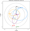 |
Figure 1 Positions and trajectories of STEREO-A (red), Earth (green), BepiColombo (gold), PSP (purple), and Solar Orbiter (blue) at the time of onset of the CME (16:00 UT on 2022-09-05). The coordinates of the plot are in the Heliocentric Earth Ecliptic (HEE) system. The purple star shows where PSP is located one day later. |
Data from PSP and SolO were obtained primarily from NASA’s Space Physics Data Facility (SPDF) using the CDAS (Coordinated Data Analysis System) web service. However, these data, unfortunately, are not sufficiently well curated for PSP, which has several instruments and modes for measuring the bulk properties of the plasma. Thus, for these measurements, we used the data set assembled by Romeo et al. (2023), including electron estimates for plasma number density obtained directly from the plasma team. Specifically, for PSP we used data from the fluxgate magnetometer part of the FIELDS (Bale et al., 2016) suite as well as from the Solar Probe ANalyzer-Ions (SPAN-i; Livi et al., 2022) and Solar Probe ANalyzer-Electrons (SPAN-e; Whittlesey et al., 2020) part of the Solar Wind Electrons Alphas and Protons (SWEAP; Kasper et al., 2016) investigation. For SolO, we employed data from the Solar Orbiter Magnetometer (MAG; Horbury et al., 2020) as well as the Solar Wind Analyser (SWA; Owen et al., 2020) suite.
Data from Bepi was processed and provided directly by the instrument team; however, we note that eventually, all cruise observations will be archived at the European Space Agency Planetary Science Archive (https://psa.esa.int/psa/#/pages/search). We used magnetic field magnitude and vector components in Radial Tangential Normal (RTN) coordinates from the MPO Magnetometer (MPO-MAG; Heyner et al., 2021). The bulk solar wind speed was derived from energy spectra collected by the ion spectrometer PICAM part of the Search for Exospheric Refilling and Emitted Natural Abundances (SERENA; Orsini et al., 2021) suite and was only available for a short interval on the 7th of September.
In-situ measurements at Earth (primarily from ACE) and STEREO-A were also obtained from NASA’s CDAS web service. In all cases, we focused on the bulk solar wind parameters, including speed, number density, temperature, and magnetic field vectors (from which angular orientations were derived). The plasma beta was estimated from the relevant magnetic and plasma measurements. For ACE, we used data from the Magnetic Field Experiment (MFE; Smith et al., 1998) and the Solar Wind Electron Proton Alpha Monitor (SWEPAM; McComas et al., 1998). For STEREO-A, we employed measurements from the Magnetic Field Experiment (MFE; Acuña et al., 2008), part of the In situ Measurements of Particles And CME Transients (IMPACT; Luhmann et al., 2008) suite as well as the Plasma and Suprathermal Ion Composition (PLASTIC; Galvin et al., 2008) investigation.
Although we analyze PSP data in this study, we realize that comparisons with such observations are fraught with difficulties. Primarily, our inner boundary is situated at 19R⊙, whereas PSP was located at approximately 15R⊙ during the CME encounter. Additionally, our simple model does not include a realistic magnetic field structure within the ejecta. Thus, at best, it may be able to reproduce the change in amplitude of the field within the CME. On the other hand, the model should be able to capture the structure of the shock and sheath region preceding the CME.
2.2 Model
The sunRunner3D model is based on the astrophysical MHD code, PLUTO (Mignone et al., 2007). PLUTO is a versatile astrophysical code that simulates HD, MHD, and relativistic flows in 3-D. It is optimized for studying complex astrophysical phenomena like jets, winds, and accretion flows, offering high flexibility with different numerical schemes and geometry options. Although the full code base provides many more features and capabilities than we leverage for sunRunner3D, we left the code “untouched”, relying only on user-defined boundary conditions to read in data, set the initial conditions, and generate the ICME pulses. By so doing, sunRunner3D should remain reasonably compatible with any future upgrades to PLUTO, and will not require the maintenance of a separate and ad hoc version of the code.
For a full list of features within the PLUTO modelling suite, the reader is encouraged to read the PLUTO User Guide (Mignone et al., 2007). Here, we distinguish some capabilities that likely separate the model from current heliospheric models. Primarily, this is due to the PLUTO team’s objective of creating a general-purpose code that could be widely applied across disciplines, focusing mainly on astrophysical (i.e., high-Mach) applications. First, the user can specify the type of fluid equations to solve: hydrodynamic, MHD (single fluid and ideal or resistive), and within these categories, they can be classical or relativistic. Second, the dimensionality and geometry of the computational domain are quite broad. Both 2D and 3D solutions can be made in Cartesian, cylindrical, or spherical coordinates. Although we highlight 3D spherical solutions here, the case could be made for heliospheric solutions in a 2D cylindrical system, capturing only evolution in the equatorial plane. Third, the spatial order of the integration can be set to a wide array of options: first-order (FLAT), piecewise TVD (linear), third-order weighted (WENO3 or LimO3), piecewise parabolic method (PPM, PARABOLIC), or fifth-order monotonically-preserving scheme (MP5). The choice comes with trade-offs between the accuracy of the solution and computational requirements; however, it is worth noting here that the barrier for testing any of these options is low – simply modify an argument in the definitions.h file, recompile, and run the code. In this way, we were able to identify the minimum complexity of the options required to capture the structure and evolution of shocks for the ICME runs. Fourth, a suite of time-stepping schemes is provided, including but not limited to Euler and Runge–Kutta 2nd (RK2) and 3rd order (RK3). Fifth, passive tracer particles can be introduced into the simulation domain. However, more uniquely, several particle modules are provided, including the ability to treat cosmic rays, Lagrangian particles, and dust grains. Although not explored, these could provide a path for incorporating, say, solar energetic particles in the future without the need for a separate code development effort. Sixth, and perhaps most importantly, PLUTO allows the user to define a set of user-specific parameters. These can be changed at run-time and are global in scope, meaning that they can be accessed from anywhere in the code. This is the mechanism we use to prescribe the properties of the CME, such as its speed, density, field strength, and duration. As we develop more sophisticated descriptions for the structure of the ejecta, such as the inclusion of helical or spheromak field lines within it, they can be incorporated within this framework. Seventh, thermal conduction and viscosity can be explicitly defined (or not) or can be treated using either super-time-stepping or RK-Legendre. Moreover, they can be set independently to one of these schemes. Finally, it cannot be over-emphasized how easy PLUTO is to set up and run. As we have shown, almost all modifications for creating a heliospheric model can be effectively made without modifying the underlying C code. In addition to writing specific user-defined subroutines, the only modifications necessary are to the files pluto.ini and definitions.h. Because of this, any future enhancements to the PLUTO code can be easily passed down to sunRunner3D, including any post-processing analysis and visualization routines.
Turning more specifically to the heliospheric model, the spatial domain spans from Rb = 0.093 AU (19R⊙) to 1–5 AU. In the simulations presented here, we placed the outer boundary at 1.1 AU, which is sufficient to cover the region of space where most of the in-situ spacecraft were located during the September 5, 2022 event. The algorithm is limited to modelling only the region of the solar wind that is everywhere super-Alfvénic, precluding us from moving the inner boundary to within the location of PSP (∼15R⊙). We adopt the standard time-dependent ideal MHD equations written in the conservative form: (1)
(1)
![Mathematical equation: $$ \frac{\partial {m}}{{\partial t}}+\nabla \cdot {\left[{m}\otimes {v}-{B}\otimes {B}+\mathrm{I}\left(p+\frac{{{B}}^2}{2}\right)\right]}^T=-\rho \nabla \mathrm{\Phi }+\rho {g} $$](/articles/swsc/full_html/2025/01/swsc240071/swsc240071-eq2.gif) (2)
(2)
 (3)
(3)
![Mathematical equation: $$ \frac{\partial \left({E}_t+\rho \mathrm{\Phi }\right)}{{\partial t}}+\nabla \cdot \left[\left(\frac{\rho {{v}}^2}{2}+\rho e+p+\rho \mathrm{\Phi }\right){v}+c{E}\times {B}\right]={m}\cdot {g} $$](/articles/swsc/full_html/2025/01/swsc240071/swsc240071-eq4.gif) (4)
(4)
where ρ is the mass density, m = ρv is the momentum density, v is the velocity, p is the thermal gas pressure, B is the vector magnetic field, I is the unit matrix, c is the speed of light, Φ is the gravitational potential, g is the acceleration vector, and ⊗ denotes a tensor (dyadic) product. Additionally, we impose (5)
(5)
The electric field, E is defined by: (6)
(6)
where
J
= c
∇×
B
, and η is the resistivity tensor. The total energy density, Et, is given by: (7)
(7)
Finally, the equation of state is given by: (8)
(8)
where n is the number density, T is the temperature, mu is the atomic mass unit, μ is the mean molecular weight, and kB is the Boltzmann constant. For our calculations, we employ an ideal gas law for a fully ionized plasma setting μ = 0.6 to account for a small amount of helium and set the polytropic index γ = 3/2, which mimics the effects of thermal conduction along the magnetic field, providing more reasonable estimates of the temperature at 1 AU (Totten et al., 1996).
For the results presented here, we set the available parameters such that we ignore body forces (gravity, which for solutions starting at 19R⊙ plays only a small role), use an ideal gas law, and include no explicit resistivity or thermal conduction. In terms of numerical schemes, we set the reconstruction to “LimO3”, time-stepping relies on RK3 (with tests using RK2), the divergence of B control relies on the “eight waves” technique (Powell, 1997), and a ring average of 8 (although this was turned off for the ambient background solution) without any adverse effects. These quantities and the rationale for choosing them are described in more detail in the PLUTO User Guide. Their use here can be further defended by noting that we experimented extensively with different combinations of options and found that they were robust and did not produce significant deviations in the solutions (e.g., de León Alanís et al., 2024).
Equations (1)–(4) are solved in a 3-D spherical coordinate system with (r,θ,ϕ) in either a corotating or inertial frame of reference. In the results presented here, we used a corotating system to generate the steady-state ambient solar wind solution but then switched to the inertial frame to initiate the ICME, which allows for easier comparisons with in-situ measurements. In the latter case, we rotated the ambient boundary conditions in longitude at a rate corresponding to the rotation rate of the solar equator, Ωc = 2π/25.38 days. This method is similar to the approaches adopted by other heliospheric codes, such as CORHEL (e.g., Riley et al., 2012), ENLIL (e.g., Odstrcil and Pizzo, 2009) and EUHFORIA (e.g., Pomoell and Poedts, 2018).
As noted above, the MHD domain extends from 19R⊙ to 1.1 AU along the radial coordinate, 0° to 180° in co-latitude (±90° in latitude), and 0° to 360° in longitude, with a grid resolution of 251 × 181 × 360, respectively. We term this grid “medium” resolution. More extensive runs can be completed at higher resolutions in all three coordinates; however, the time to complete and the resources required to be increased substantially. Additionally, qualitatively similar results are obtained even when halving the resolutions. Since the current size requires approximately 3 h to complete on a modest multi-processor computer (32 cores), this is, we believe, the best compromise. At the inner-radial boundary, we specify the values of the radial velocity vr, the mass density, the gas pressure, and the radial component of the magnetic field Br. These are derived from a CORHEL coronal solution, all of which are available at PSI’s website (https://predsci.comwww.predsci.com). At the outer radial boundary, we set outflow boundary conditions, which allow the fluid to leave the computational domain unimpeded. We employ polar-axis boundary conditions at both latitudinal boundaries, which work in conjunction with the ring average technique to help remove time-step restrictions near a singular axis (i.e., at θ = (0, π); e.g., Zhang et al., 2019). Finally, we set periodic boundary conditions in the azimuthal direction.
In addition to several user-defined routines that interface directly with the PLUTO code, sunRunner3D includes a more user-friendly Python script for initiating runs. This script can be run from the command line. In the current “stable” release, the user specifies the following parameters: (1) density (np), radial velocity (vr), transverse magnetic field (Bϕ), and temperature (Tp) of the ambient solar wind; (2) np, vr, and Bϕ for the peak values within the ICME; and (3) the duration of the ICME (τduration). Several additional features are (or will soon be) provided in the “testing” version, including (1) choice of ICME profile (e.g., bell, box, declining profile); (2) multiple ICMEs (currently up to three ICMEs are supported); and (3) support for multiple realizations allowing ensemble solutions to be computed. For this study, we use the “stable” version of sunRunner3D.
CMEs are modelled using simple “pulses” at the inner radial boundary of the simulation (19R⊙). These pulses are modulations in the speed, density, and/or magnetic field localized in latitude–longitude (a circular profile) and lasting for some fraction of a day (being ramped up smoothly, held constant, then ramped back down to ambient values). This evades the difficult (but important) questions associated with their initiation, eruption, and early evolution; however, it allows us to efficiently explore the dynamical evolution of a wide range of pulses and using modest computational resources. A variety of profiles can specify the pulse. Here, we limit them to trapezoidal variations, which are easy to implement and represent a compromise between smoother profiles, which may not develop shocks sufficiently quickly and step-like pulses, which can generate extraneous perturbations. However, in general, the precise choice leads to quantitative rather than qualitative differences in the model results. Each of the variables (vr, np, and Bϕ) can be modulated independently in an effort to best match the structure of the CME at 19R⊙. Finally, the duration of the pulse can be set arbitrarily, which impacts the resulting evolution of the structure. To the extent possible, the boundary conditions for the pulses are guided by the available remote observations. White-light observations, for example, can be used to infer the initial speed of the CME in the corona. However, other important amplitudes, like the peak density and field strength, must be indirectly inferred. A rough estimate of the peak density, for example, can be made for events where a reliable mass of the CME can be determined. However, this cannot be done with any regularity. Additionally, in principle, estimates for the peak transverse field within the ejecta could be inferred from properties of the structure at the Sun producing the event (e.g., active region). Alternatively, we can rely on inferences drawn from the in-situ measurements of the event to specify these values; However, in such cases, we are iterating on the solution to provide a scientifically better solution. Such an approach could not be used in a forecasting environment. Nevertheless, this exercise may be useful for constraining these poorly determined parameters for future space weather applications.
For the September 5, 2022 CME, based on the analyses of Patel et al. (2023) and Paouris et al. (2023), we chose an initial CME speed of ∼2240 km s−1, a duration of 9 h (which includes a smooth ramping up and lowering over 45 min), an enhancement in the number density of ×2, and an enhancement in magnetic field strength of ×2 above background values. The CME was launched at a latitude and longitude of −40° and 295°, respectively, with a cone radius of 44°. The density and magnetic field amplitudes are based heuristically on the fact that CMEs are observed to be denser than their surroundings and carry strong fields. However, whether a ×2, ×3, or more is appropriate is difficult to ascertain. Preliminary estimates for the mass of the CME have been made (Paouris et al., 2023); however, these are intrinsically uncertain and are difficult to relate to the idealized boundary conditions we employ for the CME itself. We note that the values chosen are based on our intuition from simulating a wide range of CMEs using a variety of codes over the years (e.g., Riley and Gosling, 1998; Riley et al., 2008, 2016; Riley et al., 2021). To some extent, the last three parameters can be adjusted retrospectively to better match the observations. However, since our goal is not to exactly mimic the event but to provide a generic model result that captures the general features of this type of extreme event, we have not devoted effort to this iterative exercise. In spite of this, as a basic check, we can estimate the total mass of the modelled CME by calculating the total amount of plasma ejected through the boundary at ∼19R⊙, at a speed of ∼2240 km s−1 over a duration of 8.25 h (accounting for the effects of the ramping up and down of the pulse). Such a “cylindrical” CME would have a volume of  , where Rcme is the transverse cross-sectional area of the ejecta at ∼19R⊙, and dcme is the effective radial extent of the event. Assuming the number density of the CME was 1880 cm−3, and neglecting any contributions from helium ions, the mass of the CME, Mcme = ρcme×Vcme would be approximately 6.5×10¹³ kg, which, while high, is within the typical bounds inferred from observations (e.g., Pluta et al., 2019).
3 Results
In this section, we first analyze the available observations of the September 5, 2022, CME, beginning with a summary of the available in-situ measurements. As discussed above, the remote solar observations were used to guide the specification of the model parameters for the ICME as well as providing the boundary conditions for the ambient solar wind into which the ICME propagates, and have been discussed extensively elsewhere (Long et al., 2023; Paouris et al., 2023; Patel et al., 2023; Romeo et al., 2023). The in-situ measurements are discussed within the context of understanding where in space the various spacecraft crossed the ICME and its associated disturbance. We then describe the model results. Given the limited scope of the in-situ measurements, we focus on several important aspects of the ICME some of which were observed and others of which we can only speculate since they were present but not directly observed. Together, these are used to build a more complete picture of the event, which we argue would likely have been “extreme” had the Earth been situated directly in front of it.
3.1 Analysis of in-situ measurements
We organize and discuss the in-situ measurements as follows: PSP, SolO, Bepi, STEREO-A, and ACE. This corresponds approximately to the increasing angular distance from the apex of the CME (allowing for the fact that PSP swept westward and crossed the longitudinal position of SolO before exiting the CME). This arrangement is also roughly consistent with increasing distance from the Sun (although Bepi was slightly closer to the Sun than SolO at the time of impact at the two spacecraft).
3.1.1 PSP
The in-situ measurements from PSP have been extensively analyzed by Romeo et al. (2023), Davies et al. (2024), and Liu et al. (2024). Here, we provide a brief description and interpretation of them as they relate to the large-scale simulation results. As shown in Figure 2, the event begins with a “shock” driven by the ejecta, which was observed in situ at 17:27 UT on September 5 (solid line). Unfortunately, because the ion plasma density measurements are unreliable, we cannot claim that this is a fast-mode shock (although this is supported by the magnetic field measurements). Romeo et al. (2023) identified the start of the ICME as being at 18:02 UT, based on the proton temperature dropping to less than half the value of the expectation temperature. In Figure 2 this is shown by the dotted vertical line, which lies halfway down the decrease in field magnitude and might otherwise be associated with a compression region. It also coincides roughly with the beginning of strong, coherent rotations in the magnetic field. Romeo et al. (2023) identified the trailing edge of the ICME at 01:14 UT on September 6 (dashed line), coincident with suprathermal electron signatures indicating unidirectional flow (and the lack of closed field lines), as well as a pause in the large-scale rotation of the magnetic field. We have added two further boundaries for consideration of the trailing edge of the ejecta: (1) t = 03:00 UT (dash-dot), and (2) t = 04:50 UT (dash-dot-dot). The former better aligns with the end of the large-scale rotation of the magnetic field, particularly as viewed with ΘB as well as being at the base of the speed decrease. The latter, even more conservatively, posits that the rotation of the field is not fully complete until almost 2 h later. Our point is not to argue for one boundary or another but to suggest that its location is, at best, uncertain. Beyond this structure, the measurements are rich with other complexities. For example, around 17:30 UT, there is a crossing of what appears to be the heliospheric current sheet.
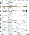 |
Figure 2 Magnetic field and plasma measurements at PSP from 2022-09-05 to 2022-09-08. From top to bottom, the panels show (a) magnetic field amplitude, (b) three components of the magnetic field (RTN); (c) and (d) the two rotation angles of the magnetic field; (e) the bulk velocity; (f) and (g) number density and temperature, as inferred from SPAN-i (blue) and SPAN-e (red); (h) plasma-β. The solid line marks the location of the fast shock driven by the CME, which is tentatively identified by the light-grey region. The leading edge of the CME is indicated by the dotted line, while three possible locations for the trailing edge are given (dashed, dash-dotted, and dash-dot-dot). |
The PSP measurements support our choice of 9 h for the duration of the simulated CME. From the data, the CME likely spans up to 8–10 h at 15R⊙, which would be moderately increased by 19R⊙. Additionally, the magnetic field amplitude and electron density measurements suggest that increases in both are reasonable.
Assuming that the bulk speed calculation is reliable, the speed decrease between 03:00 and 04:50 UT on September 6 is an interesting structure to attempt to understand. If we accept that the trailing edge of the ejecta is found at 03:00 UT, then this interval would be the most compact rarefaction region ever measured in situ. Being formed as the extremely fast CME outruns the slower material behind, it would be caused by an expansion wave that travels both back toward the Sun and outward towards the CME in front. Our simulation cannot likely capture this effect accurately since the inner boundary is set at 19R⊙, and, moreover, even if we were able to move the inner boundary to lower heights, it would not include the very early evolution at even lower heights to produce the wave. Instead, we can look at profiles at, e.g., 40R⊙ looking for qualitatively similar structures (see Sect. 3.2).
With respect to the possible expansion wave between the dashed and dash-dotted lines, a simple estimate for the distance travelled to produce such a structure can be made by noting that the leading edge of the expansion wave was travelling at 800 km s−1 and the duration of the wave was (03:00–01:14), or 106 min. Thus, assuming that the speed remained constant, we can infer that the two boundaries at either edge of the expansion wave were in contact at a near distance to the Sun of ΔR∼800×6360 km, or 7.3R⊙. Since PSP was located at ∼15R⊙, this would localize the point of separation to approximately 7.7R⊙.
A further point to note about the PSP measurements is that the ambient solar wind in front of the spacecraft was moderately less than ∼400 km s−1. Additionally, it remained low following the event. This suggests that the wind with which the CME interacted was relatively slow and dense. Finally, and as noted earlier, it is important to bear in mind that the in-situ observations at PSP do not simply represent a radial slice through the event. Instead, they are a convolution of both radial and longitudinal structures.
3.1.2 Solar Orbiter
In Figure 3, we show comparable measurements for SolO, which was located at approximately 0.7 AU (∼150R⊙) from the Sun. A fast-mode shock (solid vertical line) can be inferred from the magnetic field, speed, and temperature measurements (although density variations do not obviously support this inference). The likely interval spanned by the ejecta is marked by the dotted and dashed lines. Based on this, we suggest the ICME spanned ∼16 h. However, again, these are not conclusive for several reasons. First, unlike the event at PSP, there does not appear to be a substantial and coherent rotation in the magnetic field during the period following the shock. Second, a data gap in the currently publicly available magnetic field measurements, where the trailing edge would likely be located, complicates its identification further. We chose to place this boundary at the location of the local maximum speed, although, had we focused more on temperature variations, it could have been brought up several hours. Additionally, the location of the leading edge of the ejecta is not strongly supported by any one set of measurements. If based on temperature alone, it could be moved an hour later. The main point is that these measurements suggest a more complex set of properties for the ejecta, which, with the exception of the speed profile, do not match with those observed by PSP. Together, these suggest that the ICME was highly structured.
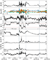 |
Figure 3 As Figure 2 except for Solar Orbiter measurements. Additionally, only proton measurements of the number density and temperature are shown. |
Finally, we remark that the wind into which SolO was propagating was of an intermediate speed (500 km s−1). Given the radial separation between PSP and SolO, it is reasonable to expect some acceleration from 15R⊙ to 0.7 au; thus, it is possible that the spacecraft was sampling similar parcels of wind. The counterargument is that the wind’s velocity at SolO is much more structured upstream with large-scale fluctuations on the size of ∼2 h (three peaks) as well as rapid fluctuations.
3.1.3 BepiColombo
In terms of progressively increasing angular separation from the source longitude of the eruption, we consider Bepi measurements next (Fig. 4). When the shock (solid black line) was encountered early on the 7th, Bepi was located at 0.63 AU from the Sun at a Carrington longitude of 340° (HEEQ longitude: −98.1°) and a heliographic latitude of −3.3°. Again, the x-axis range has been constrained to the same interval as earlier plots to allow us to track the relative time from one point of observation to another. We note several points. First, the magnetic field data support the idea that a fast-mode shock was traversed at 01:25 UT on September 7. However, given the lack of any plasma data at this time, it remains tentative. Second, there is no evidence that the spacecraft crossed a coherent helical magnetic field structure. Or, at best, it could be argued that if such a structure was present, it lasted only briefly for 4–6 h following the shock. Third, the limited speed measurements suggest that if the spacecraft were immersed in ejecta material, it was travelling at a modest speed of 500 km s−1, and we could speculate further that it was expanding, producing the declining profile. These data, however, are so limited that this inference cannot be defended rigorously. Of particular note, however, is that the shock was observed early on September 7, whereas at SolO, it was observed more than 12 h earlier, even though SolO was located 0.07 AU (∼15R⊙) farther from the Sun than Bepi. This suggests that the shock front did not lie on a spherical shell (or circle in the ecliptic plane). This could imply that the CME driving the shock was inhomogeneous in its transverse structure or that the overall shape of the shock was more parabolic, where the front falls away more rapidly if there is no driver radially underneath it. Given the (albeit limited) lack of evidence for any flux rope structure behind the shock, this suggests that the latter explanation may be correct.
 |
Figure 4 As Figure 2 except for BepiColombo measurements. Additionally, the limited bulk solar wind speed is inferred from PICAM Solar Wind mode, which scans from 250 to 2800 eV. |
3.1.4 STEREO-A and ACE
For completeness, we show comparable plots for in-situ measurements made at STEREO-A (Fig. 5) and Earth (Fig. 6). Both locations were effectively on the opposite side of the Sun from the direction of propagation of the September 5 2022 ICME, with STEREO-A being marginally closer. Although the two profiles at 1 AU are qualitatively different, we see no evidence that any part of the ICME’s disturbance propagated so far in the transverse direction as to be observable by either spacecraft. Assuming at least a 24-h transit period from, say, the location of PSP (Paouris et al., 2023), the ICME and its associated disturbance could be anticipated to arrive after 17:30 UT on September 6. There is no evidence of any compression in the field or density measurements in these data, suggesting the presence of a fast wave/shock, and there’s certainly no evidence of the spacecraft intercepting ejecta material (such as a coherent rotation in the field). Given that the ICME was not observed until 01:25 UT on September 7 at Bepi, we might further anticipate an arrival even later, say (1.00–0.63) AU/600 km s−1 or 25.6 h, or after 03:00 UT on September 8. Again, there is no evidence of any signature of the ICME on either the 8th or 9th of September. In fact, the solar wind observed during this entire time was remarkably quiescent with an essentially declining and then flat speed profile of ∼500–600 km s−1, and no anomalous variations in field strength, density, or temperature.
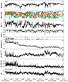 |
Figure 5 As Figure 2 except for STEREO-A measurements. Additionally, only proton measurements of the number density and temperature are shown. |
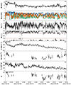 |
Figure 6 As Figure 2 except for ACE measurements. again, only proton measurements of the number density and temperature are shown. |
3.2 Model results
3.2.1 Global model properties
We begin our analysis of the model results by considering the evolution of the ICME in the equatorial plane as it propagates through the inner heliosphere. In Figure 7, we show (a) speed, (b) radial magnetic field, (c) scaled density, and (d) the logarithm of thermal pressure at a time of 20 h after the launch of the CME from the inner boundary. The coloured circles mark the nominal location of the spacecraft at this time using the same colours as in Figure 1, illustrating the key features that: (1) Earth and STA were on the opposite side of the heliosphere to the ICME; (2) Parker was located close to the apex of the ICME, but inside the inner boundary of the simulation; and (3) SolO and Bepi bounded the western and eastern edges of the disturbance driven by the ejecta.
 |
Figure 7 Equatorial slices of (a) speed (km s−1), (b) scaled (×r2) radial magnetic field (Br[nT]), (c) scaled (×r2) density (cm−3), and (d) the logarithm of thermal Pressure (PLUTO code units) at a time of 20 h since the launch of the CME. The radial traces mark radial slices equally spaced in longitude, and the coloured circles mark the nominal locations of the spacecraft at this time using the same colours as in Figure 1. |
Although the central axis of the ejecta was directed substantially away from the heliographic equator, the ICME still displays maximum radial speeds of 2300 km s−1 in the equatorial plane. The ejecta drives a strong forward shock in front of it, which stretches transversely well beyond the initial size of the ejecta. The shock has become structured as it propagates through the inhomogeneous ambient solar wind ahead. In particular, where it travels through slower and denser wind, it has decelerated. On the other hand, where the wind ahead is faster and more tenuous, the shock is free to increase in speed. Behind the ejecta, an expansion wave has developed, which propagates both back toward the Sun and into the trailing edge of the ICME (e.g. Hundhausen, 1973). Finally, we note that a second wave has developed in front of the high-speed “mesa” (broad red region, longitudinal range: 285°–310°). Moving clockwise, the shock is more of a steepened wave. Comparison with the density profile in (c) demonstrates that this is a reverse shock (or wave) driven by the initial compression of plasma ahead of the CME. In fact, in general, we can interpret many dynamical features of fast CMEs by identifying four distinct waves, two bounding the compression region and two bounding the rarefaction region. The two fast-mode waves propagate away from the growing compression region, with the forward wave steepening into a shock relatively quickly. The other fast-mode wave propagates back toward the Sun, but due to the super-Alfvénic flow of the ambient wind, this wave, too, moves away from the Sun. Often, this wave ploughs into the forward expansion wave from the developing rarefaction region and is, at least partially, obliterated (Gosling et al., 1995; Riley, 1999).
In Figure 7(b), we show the radial component of the magnetic field. Since the ICME does not contain an embedded flux rope, the structure of the field within the ICME must be interpreted with caution. Focusing instead on the processing of the ambient solar wind by the ICME, we note how the ejecta has broken up the otherwise Archimedean spirals. This is illustrated more clearly in panel (c), which shows density scaled by r2 to account for the spherical expansion of the solar wind. Two regions of compression are located at the two flanks, which happen to coincide with the location of high-density spiral arms. Again, the effect of the ejecta is to disrupt the overall Parker spiral pattern in this hemisphere. The region of highest compression lies roughly within the central longitudinal portion of the ICME as expected. Panel (d) illustrates the global extent of the disturbance, showing that it arcs around almost 180° in longitude. Of note, too, is how the observed structure would be sensitive to the observer’s precise location. Consider, for example, the radial traces within the central region behind the ejecta, containing the lowest pressure. Taking the two traces separated by only a few degrees in longitude, one spacecraft would measure a strong region of low pressure following the shock and sheath region, while the next would not.
These effects are captured in more detail in Figure 8, which documents the radial evolution of the ejecta in the equatorial plane at 10, 15, and 20 h. Traces corresponding to the lines drawn in Figure 7 are shown as a function of radial distance from the Sun to 1 AU at various helio-longitudes (as indicated in the legend). The colour-coding is the same as that in Figure 7. We note that the CME and its associated disturbance have modified the structure of the ambient solar wind over more than 90°. Generally, we can see the classic two-step pattern with a fast-forward shock at the leading edge of the compression and a reverse wave or shock at the trailing edge. This is then followed by a plateau of the highest speed wind, marking the actual ejecta. The declining speed profile behind this plateau represents a rarefaction region as the escaping ejecta sweeps up and attempts to outrun the slower plasma that was in its path.
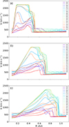 |
Figure 8 Radial velocity (km s−1) as a function of heliocentric distance (AU) for the traces marked in Figure 7 but at the times of (a) 10 h, (b) 15 h, and (c) 20 h. The profiles are colour-coded according to the same colours as in Figure 7, with the legend providing the numerical integer values. |
As the leading edge of the disturbance moves from 0.5 AU (Fig. 8(a)) to 0.7 AU (Fig. 8(b)) and finally to ∼1 AU (Fig. 8(c)), the erosion of the plateau can be seen, together with the interaction of the forward expansion wave and reverse-compression wave. Focusing on Figure 8(c), we can make several points. First, there is a large difference in the profile depending on the longitudinal position of the observer. Second, there is a significant radial separation in the position of the forward compression wave/shock, which translates into large differences in the arrival time of the shock/wave at 1 AU. Third, the rarefaction region created by the ICME is substantial. For the profiles at ∼300°, it stretches all the way from 0.2 AU to 0.7 AU.
Turning our attention to the ejecta’s evolution in the meridional plane, in Figure 9, we show (a) speed, (b) radial magnetic field, and (c) scaled density at a time of 20 h. Again, the coloured dots indicate the projected location of the spacecraft in this plane; although note that they were, in reality, separated substantially in longitude and, hence, did not experience the fluctuations shown here. We include them here primarily to highlight that Bepi and STA were located at comparable latitudes in the northern hemisphere and thus farther from the central axis than Bepi and SolO, which were both situated at similar southern latitudes. Several points are worth noting. First, the disturbance spans from ∼10°N latitude to beyond the southern pole. Based on density, the disturbance is strongest in the southern polar regions. This high compression was amplified by the slower, denser ambient solar wind into which the ICME propagated. Second, and related to this, although the ICME’s signal is strong in the equator, spacecraft located within the ecliptic plane only encountered the event at its flanks. Third, there are interesting double-peaked speed profiles at latitudes centred on ∼5°S and ∼70°S, coinciding with the compression “loops” seen in both the density and radial magnetic field panels.
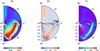 |
Figure 9 Meridional slices of (a) speed (km s−1), (b) scaled (×r2) radial magnetic field (Br[nT]), and (c) scaled (×r2) density (cm−3) at a time of 20 h. A movie of the evolution of the ICME can be found in the electronic version. |
3.2.2 Comparison with observations
As already noted, this simulation was designed to be generic in the sense of using information on the large-scale initial properties of the event (speed, width, direction of propagation) to construct a global picture of the CME and its associated disturbance. We did not perform any iterations to match the output with the available in-situ observations. However, it is instructive to compare the model time series at the approximate locations of PSP, SolO, Bepi, STEREO-A, and Earth to validate the results qualitatively. Additionally, we can make a direct comparison of the speed at SolO with the model results, which is the most meaningful.
Returning to the model results in the equatorial plane, we can view these profiles as time series from the perspective of an observer at 31R⊙, 0.7, and 1 AU, positioned at each of the helio-longitudes marked in Figure 7. These are relevant to the observations at PSP (which was at 15R⊙, that is, within the inner boundary of the calculation), SolO, and Bepi (which were at 0.7 and 0.6 AU, respectively), as well as STEREO-A and ACE (which were located at 1 AU). The first is shown in Figure 10(a). These were obtained by flying a hypothetical spacecraft through each time-step of the simulation outputted to disk; thus, the lack of sharpness in the shocks is more an artefact of capturing only a fraction of the output for visualization purposes. A future feature for the sunRunner3D suite is to include predefined observers at different locations to capture time-series profiles at the full time-step resolution of the code.
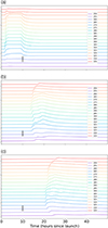 |
Figure 10 Stack plot showing radial velocity as a function of time at (a) 31R⊙, (b) 0.7 AU (orbital distance of SolO, and slightly farther away than the location of BepiColombo, at the time of the ICME), and (c) 1 AU (the orbital distance of STEREO-A and ACE), for the traces marked in Figure 7. The longitude (in degrees) of the traces is shown in the legend. Each profile is displaced by the preceding one by 1200 km/s. |
At 31R⊙, the central profiles show a very simple structure with a forward–reverse wave pair (not yet steepened into shocks), followed by a flat speed profile, and then the early phase of an expansion wave. We can compare these profiles with PSP observations (Fig. 2 acknowledging that (1) PSP was located at ∼15R⊙, and not 31R⊙, and (2) PSP’s trajectory was a contribution of longitudinal and radial variations, not simply measurements at one fixed location). Comparison with the observed speed profile is qualitatively similar in the sense that (1) there is a flat speed profile throughout the CME; (2) the duration of the CME is approximately 10 h; and (3) the expansion wave lasts several hours. However, the most notable difference is that the forward shock at the leading edge of the disturbance is much stronger, and there is no evidence of a reverse shock in the observations.
At 0.7 AU (Fig. 10(b)), the box-like profiles nearer the Sun have evolved substantially. At the apex of the ICME, the forward and reverse shocks have separated, still bounding the compression region. The forward shock is over 1000 km s−1 above the upstream ambient solar wind speed. However, far from the apex, only a steepened wave is present. None of the profiles match the SolO speed profile exactly. There is, for example, no evidence of a reverse shock/wave in the observations. However, these traces do not account for the exact trajectory of the spacecraft through the ejecta, and we will return to a more direct comparison later.
Traces at 1 AU are shown in Figure 10(c). Moving from the central traces away, we note that the forward shock weakens into a steepened wave. It is also worth pointing out that arrival time increases with distance from the apex of the ejecta. In fact, while the central portion of the shock front arrives at ∼19 h, at the flanks, it arrives more than 10 h later. The shape of the profile indicates the presence of forward/reverse shocks, bounding the compression changes substantially from one trace to the next, highlighting the difficulty of reproducing specific in-situ measurements. Unfortunately, at least from a scientific perspective, no spacecraft was situated at 1 AU directly in front of the CME, hence we cannot compare these model results with measurements. On the other hand, we can speculate this been a “direct hit” at Earth, it would likely have arrived within 19 h following the launch, with plasma speeds still exceeding 2300 km s−1.
For completeness, in Figure 11, we show time profiles at 1 AU for the latitudinal slices marked in Figure 9. The second trace from the bottom summarizes the equatorial profile at 1 AU, with the two on either side showing substantial variability ±5° about this. As noted previously, the disturbance covered the entire southern hemisphere and was centred at −40°. The profiles capture similar features, including an F shock (+5°) as well as F/R shock pairs at higher latitudes and more complicated interactions at more southern latitudes as the CME disturbance interacts with the structured ambient solar wind. At the most southern latitudes, the profile returns to a simple F/R wave pair and expansion wave as the slices intercept only the disturbance but not the driving ICME.
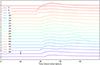 |
Figure 11 As Figure 10(c), i.e., at 1 AU, except for the traces marked in Figure 9. In this case, each profile is displaced by the preceding one by 2000 km s−1. |
In an effort to make a more direct comparison with spacecraft observations, in Figure 12, we have reproduced the speed profile at SolO by flying along the spacecraft’s trajectory within the simulation domain. We focus on SolO since it was (1) closest to the apex of the ejecta, (2) located sufficiently far from the source to see evolutionary effects, and (3) also within the bounds of the simulation region. These constraints were not met by the other spacecraft. For example, PSP was located more on the flanks of the event, and its trajectory was inside the inner boundary of the calculation. STA and Earth, in contrast, were located almost 180° to the direction of propagation. Finally, Bepi, which lay almost at quadrature, was not able to provide any usable plasma profiles during the event. Since the model CME did not contain an embedded flux rope, a comparison with the observed field components at Bepi would also not be particularly valuable.
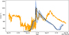 |
Figure 12 Comparison of modelled (black) and observed (orange) values of solar wind speed at the location of SolO. The blue interval marks the range of values 3° around the spacecraft trajectory, providing a measure of uncertainty in the model results. A time shift of 05:50:24 has been applied to the model results. |
The comparison at SolO reveals several important points. First, the modelled upstream solar wind speed is substantially lower than was observed (300 km s−1 versus 450 km s−1), a result of the ambient solar wind model not accurately capturing the observed solar wind into which the CME propagated. This had the effect of slowing down the modelled ejecta more than the observed one, likely the cause of us having to shift the profile by 5.84 h to make the comparison better. Second, at the back of the event, the model only produces a single declining speed profile (an expansion wave), connecting the faster wind in the CME with the slower following wind. In reality, there was a second high-speed flow presumably caused by a second CME that was not modelled. Overall, however, the speed profile around the shock front is reasonably well matched and, given the generic nature of the calculation, provides sufficient validation of the model results to support the basic large-scale global structure of the ejecta that passed over the various spacecraft.
A final point worth making concerns the shape of the propagating shock front. From the observations, we infer that the shock reached SolO at ∼0.7 AU more than 13 h before it arrived at Bepi, which was located closer to the Sun at ∼0.63 AU. This is supported by the large-scale structure of the shock front shown in Figure 7. At this time, the shock had already passed over SolO (and was more than 0.1 AU in front at this point) but was still behind Bepi (by more than 0.1 AU). From panel (a), in particular, we infer that Bepi only intercepted the shock at its easternmost edge, while SolO intercepted the shock and ejecta towards its western edge but closer to its centre.
4 Summary and discussion
In this study, we have developed a generic simulation aimed at capturing the essential dynamical properties of the September 5, 2022 ICME. Based on the limited but available properties of the ejecta as it passed through the corona, we were able to develop a pulse profile that mimicked the initial properties of the event as it propagated through the upper corona and passed over three in-situ spacecraft. Our model results, while instructive for exploring what might have been seen had a spacecraft been directly in its path, are also speculative in the sense that the limited in-situ measurements only confirm the general picture painted by the model results. However, we previously demonstrated (Riley and Ben-Nun, 2022) how a 1-D version of this code is capable of reproducing slow, fast, and even extreme ICME profiles when their initial properties can be sufficiently constrained, giving us further confidence in the basic features of the global model results.
The model results suggest that if the ejecta had been launched directly along the Sun-Earth line, it would have been an extreme event on the scale of September 1, 1859, or July 23, 2012 events (although this is based exclusively on the inferred speeds, and would require knowledge about the amplitude and duration of southward magnetic fields within the ejecta to substantiate). The likely consequences of such impacts in our technology-dependent society have been explored in several studies (e.g., Tsurutani et al., 2003; Baker, 2012; Eastwood et al., 2017), and could have included power grid failures, communication disruptions, and satellite damage, amongst other consequences. What is intriguing about our modelled event is that the solar wind was not first preconditioned with a precursor CME, which was likely the case for these two other examples (e.g., Temmer and Nitta, 2015). Thus, we suggest that while a “perfect storm” may benefit from a precursor, it is not a necessary condition to produce an extreme event. We caution, however, that our modelled CME did not include a realistic magnetic field within the ejecta; thus, it is possible that the effects of the event may have been muted if the flux rope within did not contain strong and persistent southward magnetic fields, which are required to generate the strongest geomagnetic storms.
The current version of sunRunner3D contains a number of limitations, all of which we plan to address in future updates. First, there is no option to embed hypothetical spacecraft within the simulation domain. This limitation is circumvented by outputting the 3-D variables at sufficiently high temporal resolution and interpolating through the results as a function of time and space. This requires a relatively large amount of storage, given that only a single trace is ultimately produced. This could be improved upon by collecting high-time resolution information at fixed spatial points within the domain, or even better; the user could supply a time-dependent trajectory mimicking the movement of a specific spacecraft during the run. The latter option would be ideal for cases involving PSP encounters, where the spacecraft sweeps rapidly across longitude. Second, tracer particles cannot be easily specified within the sunRunner3D setup. Such a feature is useful for marking the boundary of structures, like CMEs, allowing the user to more easily track their edges as they propagate and evolve in the inner heliosphere. There is, however, a feature in PLUTO (NTRACER option), which could be adapted for this purpose. Third, the inner radial boundary cannot yet be driven by a set of time-dependent magnetofluid variables. CME calculations are driven by specifying an equilibrium solution that is rotated at the solar rotation rate, and a pulse-like CME, which is described by a set of standard model parameters, is introduced at the boundary. A more general prescription would be to allow the user to provide a sequence of 2-D slices of v, B, np, and Tp, for example. These could be extracted from previously-run coronal simulation or, in the future, perhaps derived empirically from observations of available remotely-observed quantities in the upper corona (e.g., white-light observations, Faraday rotation measures, etc.). Fourth, there are currently limited post-processing tools for users to easily interact with the results. All of the available PLUTO tools (written in either Python or IDL) can be used to analyze and visualize the data. We also recently published a GitHub repository, pysunrunner (PSI, 2024), which allows the user to produce visualizations such as those found in this study. For more widespread adoption of this tool by the heliospheric community, this should be further developed into a comprehensive set of tools, including, for example, Jupyter notebooks. Additionally, post-processing scripts that automatically create a set of standard visuals from each run would make the task of interacting with model results less arduous.
Despite these limitations, the code underlying the sunRunner3D framework brings a set of features that are likely unmatched by any single currently available community heliospheric model (see Sect. 2.2). While many, if not all, can be found in any specific heliospheric model implementation, no single model provides access to all of them (at least a model that is generally available to the community). Thus, we believe that sunRunner3D provides an excellent base for future heliospheric modellers to explore a wide range of scientific questions.
A natural avenue for future research of the September 5, 2022, CME is to attempt to model the eruption process more self-consistently and then propagate the resulting flux rope through the extended corona and out to 1 AU. These types of simulations have been applied to extreme events in the past (e.g., Manchester et al., 2008; To¨ro¨k et al., 2018), but require considerably more effort to set up, run, post-process, and interpret. However, they are clearly valuable, being able to address scientific questions that are not possible with the empirical approach described here. One study underway (Palmerio et al., 2023) is using the CORHEL framework to do just this. Preliminary results suggest that the complicated observed in-situ measurements may be caused, at least in part, by the complex eruption profile associated with the neutral line threading AR 13088. The PLUTO code has also been used to model ICMEs with embedded flux ropes. The SWASTi-CME model (Mayank et al., 2024) integrates a magnetized flux rope CME model within a pulse similar to that used to drive the simulation presented here. Future studies using the SWASTi-CME code or implementing an equivalent description within sunRunner3D may better match the observations by various spacecraft. At the least, they could be used to explore the evolution of ad hoc, embedded flux ropes as a methodology for bridging the gap between the more self-consistent approaches that include the evolution through the low corona and the simpler “pulse” approaches presented here.
In closing, we reiterate the main points of this study: (1) to introduce a new yet simple global MHD model (sunRunner3D capable of modelling ICMEs from the upper corona to 1–5 AU, and (2) apply it to interpret a set of in-situ measurements associated with the September 5, 2022 ICME. sunRunner3D requires modest computational resources and can be easily set up by non-specialists. By retaining all of the sophisticated numerical schemes built into the underlying code (PLUTO) while avoiding any explicit modification of it, users can explore a wide range of options for testing different methodologies. For example, adaptive mesh refinement (AMR) techniques could be included, as well as future improvements to the code (e.g., GPU acceleration). We demonstrated the use of sunRunner3D by developing a model solution that captures the essential (but not all) features of the September 5, 2022 CME. The results presented here support inferences drawn from other studies of this event, such as its extreme properties, and additionally, the view of the global structure of the event provides additional information for the CME’s structure, which was not obviously captured by any of the available observations.
Acknowledgments
The authors at PSI gratefully acknowledge support from NASA (grants no. 80NSSC20K0695, 80NSSC20K1274, 80NSSC20K1285, 80NSSC22K0349, 80NSSC23K0258, and 80NSSC24K1108), the PSP WISPR contract NNG11EK11I to NRL (under subcontract N00173-24-C-0004 to PSI), and NSF’s PREEVENTS program (grant no. ICER-1854790). J.J.G.-A. acknowledges the “Consejo Nacional de Humanidades, Ciencias y Tecnologías (CONAHCYT)” 319216 project “Modalidad: Paradigmas y Controversias de la Ciencia 2022”, for the financial support of this work. A.K. acknowledges financial support from NASA NNN06AA01C (PSP EPI-Lo) contract and from NASA HTM grant 80NSSC24K0071. B.S.-C. acknowledges support from the UK-STFC Ernest Rutherford fellowship ST/V004115/1 and the BepiColombo guest investigator grant ST/Y000439/1. A.M. acknowledges support from the ASI-INAF agreement no. 2018- 8-HH.1-2022 for BEPICOLOMBO SERENA . The FIELDS and SWEAP experiments on the Parker spacecraft was designed and developed under NASA contract NNN06AA01C. We acknowledge the NASA Parker Solar Probe Mission and the SWEAP team led by J. Kasper for use of data. The authors are grateful to the developers of the PLUTO software, which provides a general and sophisticated interface for the numerical solution of mixed hyperbolic/parabolic systems of partial differential equations (conservation laws) targeting high Mach number flows in astrophysical fluid dynamics (Mignone et al., 2007). All data and code used to generate the results of this study are being made available as part of a GitHub repository https://github.com/predsci/sunRunner3D-manuscript. The datasets used were retrieved from NASA’s SPDF facility (https://spdf.gsfc.nasa.gov/). sunRunner3D is based on the astrophysical code, PLUTO, which can be obtained from: http://plutocode.ph.unito.it/. The editor thanks Volker Bothmer and an anonymous reviewer for their assistance in evaluating this paper.
References
- Acuña MH, Curtis D, Scheifele JL, Russell CT, Schroeder P, Szabo A, Luhmann JG. 2008. The STEREO/IMPACT magnetic field experiment. Space Sci Rev 136(1–4): 203–226. https://doi.org/10.1007/s11214-007-9259-2. [CrossRef] [Google Scholar]
- Al-Haddad N, Nieves-Chinchilla T, Savani NP, Lugaz N, Roussev II. 2018. Fitting and reconstruction of thirteen simple coronal mass ejections. Sol Phys 293(5): 73. https://doi.org/10.1007/s11207-018-1288-3. [CrossRef] [Google Scholar]
- Baker DN. 2012. Extreme space weather: forecasting behavior of a nonlinear dynamical system. Geophys Monogr Ser 196: 255–265. https://doi.org/10.1029/2011GM001075. [Google Scholar]
- Bale SD, Goetz K, Harvey PR, Turin P, Bonnell JW, et al. 2016. The FIELDS instrument suite for solar probe plus. Measuring the coronal plasma and magnetic field, plasma waves and turbulence, and radio signatures of solar transients. Space Sci Rev 204(1–4): 49–82. https://doi.org/10.1007/s11214-016-0244-5. [CrossRef] [Google Scholar]
- Benkhoff J, Murakami G, Baumjohann W, Besse S, Bunce E, et al. 2021. BepiColombo – mission overview and science goals. Space Sci Rev 217(8): 90. https://doi.org/10.1007/s11214-021-00861-4. [CrossRef] [Google Scholar]
- Cohen CMS, Leske RA, Christian ER, Cummings AC, de Nolfo GA, et al. 2024. Observations of the 2022 September 5 solar energetic particle event at 15 solar radii. Astrophys J 966(2): 148. https://doi.org/10.3847/1538-4357/ad37f8. [CrossRef] [Google Scholar]
- Davies EE, Rüdisser HT, Amerstorfer UV, Möstl C, Bauer M, et al. 2024. Flux rope modeling of the 2022 September 5 coronal mass ejection observed by Parker Solar Probe and Solar Orbiter from 0.07 to 0.69 au. Astrophys J 973(1): 51. https://doi.org/10.3847/1538-4357/ad64cb. [CrossRef] [Google Scholar]
- de León Alanís LA, González-Avilés JJ, Riley P, Ben-Nun M. 2024. Investigating the effects of numerical algorithms on global magnetohydrodynamics simulations of solar wind in the inner heliosphere. Revista Mexicana de Fisica 70(3): 031501. https://doi.org/10.31349/RevMexFis.70.031501. [Google Scholar]
- Ding Z, Li G, Mason G, Poedts S, Kouloumvakos A, Ho G, Wijsen N, Wimmer-Schweingruber RF, Rodríguez-Pacheco J. 2024. Modelling two energetic storm particle events observed by Solar Orbiter using the combined EUHFORIA and iPATH models. Astron Astrophys 681: A92. https://doi.org/10.1051/0004-6361/202347506. [CrossRef] [EDP Sciences] [Google Scholar]
- Domingo V, Fleck B, Poland AI. 1995. The SOHO mission: an overview. Sol Phys 162(1–2): 1–37. https://doi.org/10.1007/BF00733425. [CrossRef] [Google Scholar]
- Dryer M, Smith Z, Fry CD, Sun W, Deehr CS, Akasofu SI. 2004. Real-time shock arrival predictions during the “Halloween 2003 epoch”. Space Weather 2(9): S09001. https://doi.org/10.1029/2004SW000087. [CrossRef] [Google Scholar]
- Eastwood JP, Biffis E, Hapgood MA, Green L, Bisi MM, Bentley RD, Wicks R, McKinnell LA, Gibbs M, Burnett C. 2017. The economic impact of space weather: where do we stand? Risk Anal 37(2): 206–218. https://doi.org/10.1111/risa.12765. [CrossRef] [Google Scholar]
- Fox NJ, Velli MC, Bale SD, Decker R, Driesman A, et al. 2016. The solar probe plus mission: humanity’s first visit to our star. Space Sci Rev 204(1–4): 7–48. https://doi.org/10.1007/s11214-015-0211-6. [CrossRef] [Google Scholar]
- Galvin AB, Kistler LM, Popecki MA, Farrugia CJ, Simunac KDC, et al. 2008. The plasma and suprathermal ion composition (PLASTIC) investigation on the STEREO observatories. Space Sci Rev 136: 437–486. https://doi.org/10.1007/s11214-007-9296-x. [CrossRef] [Google Scholar]
- Gosling JT. 1990. Coronal mass ejections and magnetic flux ropes in interplanetary space. Geophys Monogr Ser 58: 343–364. https://doi.org/10.1029/GM058p0343. [Google Scholar]
- Gosling JT, McComas DJ, Phillips JL, Pizzo VJ, Goldstein BE, Forsyth RJ, Lepping RP. 1995. A CME-driven solar wind disturbance observed at both low and high heliographic latitudes. Geophys Res Lett 22(13): 1753–1756. https://doi.org/10.1029/95GL01776. [CrossRef] [Google Scholar]
- Heyner D, Auster HU, Fornaçon KH, Carr C, Richter I, et al. 2021. The BepiColombo planetary magnetometer MPO-MAG: what can we learn from the hermean magnetic field? Space Sci Rev 217(4): 52. https://doi.org/10.1007/s11214-021-00822-x. [CrossRef] [Google Scholar]
- Horbury TS, O’Brien H, Carrasco Blazquez I, Bendyk M, Brown P, et al. 2020. The Solar Orbiter magnetometer. Astron Astrophys 642: A9. https://doi.org/10.1051/0004-6361/201937257. [CrossRef] [EDP Sciences] [Google Scholar]
- Hu Q, Sonnerup B. 2002. Reconstruction of magnetic clouds in the solar wind: orientations and configurations. J Geophys Res 107(A7): SSH-10. https://doi.org/10.1029/2001JA000293. [Google Scholar]
- Hundhausen AJ. 1973. Evolution of large-scale solar wind structures beyond 1 AU. J Geophys Res 78(13): 2035. https://doi.org/10.1029/JA078i013p02035. [CrossRef] [Google Scholar]
- Hundhausen AJ. 1985. Some macroscopic properties of shock waves in the heliosphere. Geophys Monogr Ser 34: 37–58. https://doi.org/10.1029/GM034p0037. [Google Scholar]
- Kaiser ML, Kucera TA, Davila JM, Cyr St. OC, Guhathakurta M, Christian E. 2008. The STEREO mission: an introduction. Space Sci Rev 136: 5–16. https://doi.org/10.1007/s11214-007-9277-0. [CrossRef] [Google Scholar]
- Kasper JC, Abiad R, Austin G, Balat-Pichelin M, Bale SD, et al. 2016. Solar wind electrons alphas and protons (SWEAP) investigation: design of the solar wind and coronal plasma instrument suite for solar probe plus. Space Sci Rev 204(1–4): 131–186. https://doi.org/10.1007/s11214-015-0206-3. [CrossRef] [Google Scholar]
- Kilpua E, Koskinen HEJ, Pulkkinen TI. 2017. Coronal mass ejections and their sheath regions in interplanetary space. Living Rev Sol Phys 14(1): 5. https://doi.org/10.1007/s41116-017-0009-6. [CrossRef] [Google Scholar]
- Ledvina VE, Palmerio E, Kay C, Al-Haddad N, Riley P. 2023. Modeling CME encounters at Parker Solar Probe with OSPREI: dependence on photospheric and coronal conditions. Astron Astrophys 673: A96. [CrossRef] [EDP Sciences] [Google Scholar]
- Liu YD, Zhu B, Ran H, Hu H, Liu M, Zhao X, Wang R, Stevens ML, Bale SD. 2024. Direct in situ measurements of a fast coronal mass ejection and associated structures in the corona. Astrophys J 963(2): 85. https://doi.org/10.3847/1538-4357/ad1e56. [CrossRef] [Google Scholar]
- Livi R, Larson DE, Kasper JC, Abiad R, Case AW, et al. 2022. The Solar Probe ANalyzer-ions on the Parker Solar Probe. Astrophys J 938(2): 138. https://doi.org/10.3847/1538-4357/ac93f5. [CrossRef] [Google Scholar]
- Long DM, Green LM, Pecora F, Brooks DH, Strecker H, et al. 2023. The eruption of a magnetic flux rope observed by Solar Orbiter and Parker Solar Probe. Astrophys J 955(2): 152. https://doi.org/10.3847/1538-4357/acefd5. [CrossRef] [Google Scholar]
- Luhmann JG, Curtis DW, Schroeder P, McCauley J, Lin RP, et al. 2008. STEREO IMPACT investigation goals, measurements, and data products overview. Space Sci Rev 136: 117–184. https://doi.org/10.1007/s11214-007-9170-x. [CrossRef] [Google Scholar]
- Manchester I, Ward B, Vourlidas A, Tóth G, Lugaz N, Roussev II, Sokolov IV, Gombosi TI, De Zeeuw DL, Opher M. 2008. Three-dimensional MHD simulation of the 2003 October 28 coronal mass ejection: comparison with LASCO coronagraph observations. Astrophys J 684(2): 1448–1460. https://doi.org/10.1086/590231. [CrossRef] [Google Scholar]
- Manchester WB, Gombosi TI, Roussev I, de Zeeuw DL, Sokolov IV, Powell KG, Tóth G, Opher M. 2004. Three-dimensional MHD simulation of a flux rope driven CME. J Geophys Res (Space Phys) 109(A1): A01102. https://doi.org/10.1029/2002JA009672. [Google Scholar]
- Mayank P, Vaidya B, Mishra W, Chakrabarty D. 2024. SWASTi-CME: a physics-based model to study coronal mass ejection evolution and its interaction with solar wind. Astrophys J Suppl 270(1): 10. https://doi.org/10.3847/1538-4365/ad08c7. [CrossRef] [Google Scholar]
- McComas DJ, Riley P, Gosling JT, Balogh A, Forsyth R. 1998. Ulysses’ rapid crossing of the polar coronal hole boundary. J Geophys Res 103(A2): 1955–1967. https://doi.org/10.1029/97JA01459. [CrossRef] [Google Scholar]
- Mignone A, Bodo G, Massaglia S, Matsakos T, Tesileanu O, Zanni C, Ferrari A. 2007. PLUTO: a numerical code for computational astrophysics. Astrophys J Suppl 170(1): 228–242. https://doi.org/10.1086/513316. [CrossRef] [Google Scholar]
- Müller D, Cyr St. OC, Zouganelis I, Gilbert HR, Marsden R, et al. 2020. The Solar Orbiter mission. Science overview. Astron Astrophys 642: A1. https://doi.org/10.1051/0004-6361/202038467. [CrossRef] [EDP Sciences] [Google Scholar]
- Odstrcil D. 2009. Numerical simulation of interplanetary disturbances. In: Pogorelov NV, Audit E, Colella P, Zank GP (Eds.), Numerical modeling of space plasma flows: ASTRONUM-2008, vol. 406 of Astronomical society of the pacific conference series, p. 141. [Google Scholar]
- Odstrcil D, Pizzo VJ. 2009. Numerical heliospheric simulations as assisting tool for interpretation of observations by STEREO heliospheric imagers. Sol Phys 259: 297–309. https://doi.org/10.1007/s11207-009-9449-z. [CrossRef] [Google Scholar]
- Ogilvie KW, Desch MD. 1997. The wind spacecraft and its early scientific results. Adv Space Res 20(4–5): 559–568. https://doi.org/10.1016/S0273-1177(97)00439-0. [CrossRef] [Google Scholar]
- Orsini S, Livi SA, Lichtenegger H, Barabash S, Milillo A, et al. 2021. SERENA: particle instrument suite for determining the sun-mercury interaction from BepiColombo. Space Sci Rev 217(1): 11. https://doi.org/10.1007/s11214-020-00787-3. [CrossRef] [Google Scholar]
- Owen CJ, Bruno R, Livi S, Louarn P, Al Janabi K, et al. 2020. The Solar Orbiter solar wind analyser (SWA) suite. Astron Astrophys 642: A16. https://doi.org/10.1051/0004-6361/201937259. [CrossRef] [EDP Sciences] [Google Scholar]
- Owens M, Lang M, Barnard L, Riley P, Ben-Nun M, Scott CJ, Lockwood M, Reiss MA, Arge CN, Gonzi S. 2020. A computationally efficient, time-dependent model of the solar wind for use as a surrogate to three-dimensional numerical magnetohydrodynamic simulations. Sol Phys 295(3): 43. https://doi.org/10.1007/s11207-020-01605-3. [CrossRef] [Google Scholar]
- Palmerio E, Carcaboso F, Khoo LY, Salman TM, Sánchez-Cano B, et al. 2024. On the mesoscale structure of coronal mass ejections at Mercury’s Orbit: BepiColombo and Parker Solar Probe observations. Astrophys J 963(2): 108. https://doi.org/10.3847/1538-4357/ad1ab4. [CrossRef] [Google Scholar]
- Palmerio E, Linker J, Downs C, Torok T, Riley P, Caplan RM, Linton M. 2023. Global modelling of the labor day CME observed in the corona by Parker Solar Probe. In: AGU fall meeting abstracts, vol. 2023, pp. SH31D–3004. [Google Scholar]
- Paouris E, Vourlidas A, Kouloumvakos A, Papaioannou A, Jagarlamudi VK, Horbury T. 2023. The space weather context of the first extreme event of solar cycle 25, on 2022 September 5. Astrophys J 956(1): 58. https://doi.org/10.3847/1538-4357/acf30f. [CrossRef] [Google Scholar]
- Patel R, West MJ, Seaton DB, Hess P, Niembro T, Reeves KK. 2023. The closest view of a fast coronal mass ejection: how faulty assumptions near perihelion lead to unrealistic interpretations of PSP/WISPR observations. Astrophys J Lett 955(1): L1. https://doi.org/10.3847/2041-8213/acf2f0. [CrossRef] [Google Scholar]
- Pesnell WD, Thompson BJ, Chamberlin PC. 2012. The solar dynamics observatory (SDO). Sol Phys 275(1–2): 3–15. https://doi.org/10.1007/s11207-011-9841-3. [Google Scholar]
- Pizzo VJ, de Koning C, Cash M, Millward G, Biesecker DA, Puga L, Codrescu M, Odstrcil D. 2015. Theoretical basis for operational ensemble forecasting of coronal mass ejections. Space Weather 13(10): 676–697. https://doi.org/10.1002/2015SW001221. [CrossRef] [Google Scholar]
- Pluta A, Mrotzek N, Vourlidas A, Bothmer V, Savani N. 2019. Combined geometrical modelling and white-light mass determination of coronal mass ejections. Astron Astrophys 623: A139. https://doi.org/10.1051/0004-6361/201833829. [CrossRef] [EDP Sciences] [Google Scholar]
- Pomoell J, Poedts S. 2018. EUHFORIA: European heliospheric forecasting information asset. J Space Weather Space Clim 8: A35. https://doi.org/10.1051/swsc/2018020. [Google Scholar]
- Powell KG. 1997. An approximate Riemann solver for magnetohydrodynamics. Springer Berlin Heidelberg, Berlin, Heidelberg, pp. 570–583. https://doi.org/10.1007/978–3-642–60543-7_23. [Google Scholar]
- PSI. 2024. pysunrunner: a python tool for running and managing solar models. https://github.com/predsci/pysunrunner. Accessed: 2024-10-02. [Google Scholar]
- Riley P. 1999. CME dynamics in a structured solar wind. In: Habbal SR, Esser R, Hollweg JV, Isenberg PA (Eds.), Solar wind nine, vol. 471 of American institute of physics conference series. AIP, pp. 131–136. https://doi.org/10.1063/1.58741. [Google Scholar]
- Riley P, Ben-Nun M. 2021. On the sources and sizes of uncertainty in predicting the arrival time of interplanetary coronal mass ejections using global MHD models. Space Weather 19(6): e2021SW002775. [NASA ADS] [CrossRef] [Google Scholar]
- Riley P, Ben-Nun M. 2022. sunRunner1D: a tool for exploring ICME evolution through the inner heliosphere. Universe 8(9): 447. https://doi.org/10.3390/universe8090447. [CrossRef] [Google Scholar]
- Riley P, Caplan RM, Downs C, Linker JA, Lionello R. 2022. Comparing and contrasting the properties of the inner heliosphere for the three most recent solar minima. J Geophys Res (Space Phys) 127(8): e30261. https://doi.org/10.1029/2022JA030261. [Google Scholar]
- Riley P, Caplan RM, Giacalone J, Lario D, Liu Y. 2016. Properties of the fast forward shock driven by the July 23 2012 extreme coronal mass ejection. Astrophys J 819: 57. https://doi.org/10.3847/0004-637X/819/1/57. [CrossRef] [Google Scholar]
- Riley P, Gosling JT. 1998. Do coronal mass ejections implode in the solar wind? Geophys Res Lett 25(9): 1529–1532. https://doi.org/10.1029/98GL01057. [CrossRef] [Google Scholar]
- Riley P, Gosling JT, Pizzo VJ. 1997. A two-dimensional simulation of the radial and latitudinal evolution of a solar wind disturbance driven by a fast, high-pressure coronal mass ejection. J Geophys Res 102(A7): 14677–14686. https://doi.org/10.1029/97JA01131. [CrossRef] [Google Scholar]
- Riley P, Linker JA, Lionello R, Mikic Z. 2012. Corotating interaction regions during the recent solar minimum: the power and limitations of global MHD modeling. J Atmos Sol Terr Phys 83: 1–10. https://doi.org/10.1016/j.jastp.2011.12.013. [CrossRef] [Google Scholar]
- Riley P, Lionello R, Caplan RM, Downs C, Linker JA, Badman ST, Stevens ML. 2021. Using Parker Solar Probe observations during the first four perihelia to constrain global magnetohydrodynamic models. Astron Astrophys 650: A19. [CrossRef] [EDP Sciences] [Google Scholar]
- Riley P, Lionello R, Mikić Z, Linker J. 2008. Using global simulations to relate the three-part structure of coronal mass ejections to in situ signatures. Astrophys J 672: 1221–1227. https://doi.org/10.1086/523893. [CrossRef] [Google Scholar]
- Rochus P, Auchère F, Berghmans D, Harra L, Schmutz W, et al. 2020. The Solar Orbiter EUI instrument: the extreme ultraviolet imager. Astron Astrophys 642: A8. https://doi.org/10.1051/0004-6361/201936663. [CrossRef] [EDP Sciences] [Google Scholar]
- Romeo OM, Braga CR, Badman ST, Larson DE, Stevens ML, et al. 2023. Near-sun in situ and remote-sensing observations of a coronal mass ejection and its effect on the heliospheric current sheet. Astrophys J 954(2): 168. https://doi.org/10.3847/1538-4357/ace62e. [CrossRef] [Google Scholar]
- Scherrer PH, Schou J, Bush RI, Kosovichev AG, Bogart RS, et al. 2012. The helioseismic and magnetic imager (HMI) investigation for the solar dynamics observatory (SDO). Sol Phys 275(1–2): 207–227. https://doi.org/10.1007/s11207-011-9834-2. [CrossRef] [Google Scholar]
- Smith CW, L’Heureux J, Ness NF, Acuña MH, Burlaga LF, Scheifele J. 1998. The ACE magnetic fields experiment. Space Sci Rev 86: 613–632. https://doi.org/10.1023/A:1005092216668. [CrossRef] [Google Scholar]
- Stone EC, Frandsen AM, Mewaldt RA, Christian ER, Margolies D, Ormes JF, Snow F. 1998. The advanced composition explorer. Space Sci Rev 86: 1–22. https://doi.org/10.1023/A:1005082526237. [CrossRef] [Google Scholar]
- Temmer M, Nitta NV. 2015. Interplanetary propagation behavior of the fast coronal mass ejection on 23 July 2012. Sol Phys 290(3): 919–932. https://doi.org/10.1007/s11207-014-0642-3. [CrossRef] [Google Scholar]
- Thernisien A. 2011. Implementation of the graduated cylindrical shell model for the three-dimensional reconstruction of coronal mass ejections. Astrophys J Suppl 194(2): 33. https://doi.org/10.1088/0067-0049/194/2/33. [CrossRef] [Google Scholar]
- Török T, Downs C, Linker JA, Lionello R, Titov VS, Mikić Z, Riley P, Caplan RM, Wijaya J. 2018. Sun-to-earth MHD simulation of the 2000 July 14 “Bastille Day” eruption. Astrophys J 856(1): 75. https://doi.org/10.3847/1538-4357/aab36d. [CrossRef] [Google Scholar]
- Totten TL, Freeman JW, Arya S. 1996. Application of the empirically derived polytropic index for the solar wind to models of solar wind propagation. J Geophys Res 101(A7): 15629–15636. https://doi.org/10.1029/96JA01019. [CrossRef] [Google Scholar]
- Trotta D, Larosa A, Nicolaou G, Horbury TS, Matteini L, et al. 2024. Properties of an interplanetary shock observed at 0.07 and 0.7 au by Parker Solar Probe and Solar Orbiter. Astrophys J 962(2): 147. https://doi.org/10.3847/1538-4357/ad187d. [CrossRef] [Google Scholar]
- Tsurutani BT, Gonzalez WD, Lakhina GS, Alex S. 2003. The extreme magnetic storm of 1–2 September 1859. J Geophys Res (Space Phys) 108(A7): 1268. https://doi.org/10.1029/2002JA009504. [Google Scholar]
- Vourlidas A, Howard RA, Plunkett SP, Korendyke CM, Thernisien AFR, et al. 2016. The wide-field imager for solar probe plus (WISPR). Space Sci Rev 204(1–4): 83–130. https://doi.org/10.1007/s11214-014-0114-y. [CrossRef] [Google Scholar]
- Weiss AJ, Möstl C, Davies EE, Amerstorfer T, Bauer M, et al. 2021. Multi-point analysis of coronal mass ejection flux ropes using combined data from Solar Orbiter, BepiColombo, and wind. Astron Astrophys 656: A13. https://doi.org/10.1051/0004-6361/202140919. [CrossRef] [EDP Sciences] [Google Scholar]
- Whittlesey PL, Larson DE, Kasper JC, Halekas J, Abatcha M, et al. 2020. The Solar Probe ANalyzers—electrons on the Parker Solar Probe. Astrophys J Suppl 246(2): 74. https://doi.org/10.3847/1538-4365/ab7370. [CrossRef] [Google Scholar]
- Winslow RM, Lugaz N, Schwadron NA, Farrugia CJ, Yu W, Raines JM, Mays ML, Galvin AB, Zurbuchen TH. 2016. Longitudinal conjunction between MESSENGER and STEREO A: development of ICME complexity through stream interactions. J Geophys Res (Space Phys) 121(7): 6092–6106. https://doi.org/10.1002/2015JA022307. [CrossRef] [Google Scholar]
- Zhang B, Sorathia KA, Lyon JG, Merkin VG, Wiltberger M. 2019. Conservative averaging-reconstruction techniques (Ring Average) for 3-D finite-volume MHD solvers with axis singularity. J Comput Phys 376: 276–294. https://doi.org/10.1016/j.jcp.2018.08.020. [CrossRef] [Google Scholar]
- Zurbuchen TH, Richardson IG. 2006. In-situ solar wind and magnetic field signatures of interplanetary coronal mass ejections. Space Sci Rev 123: 31–43. https://doi.org/10.1007/s11214-006-9010-4. [CrossRef] [Google Scholar]
Cite this article as: Riley P, Ben-Nun M, González-Avilés J, Palmerio E, Török T, et al. 2025. Understanding the global structure of the September 5, 2022, coronal mass ejection using sunRunner3D. J. Space Weather Space Clim. 15, 17. https://doi.org/10.1051/swsc/2025010.
All Figures
|
Figure 1 Positions and trajectories of STEREO-A (red), Earth (green), BepiColombo (gold), PSP (purple), and Solar Orbiter (blue) at the time of onset of the CME (16:00 UT on 2022-09-05). The coordinates of the plot are in the Heliocentric Earth Ecliptic (HEE) system. The purple star shows where PSP is located one day later. |
| In the text | |
|
Figure 2 Magnetic field and plasma measurements at PSP from 2022-09-05 to 2022-09-08. From top to bottom, the panels show (a) magnetic field amplitude, (b) three components of the magnetic field (RTN); (c) and (d) the two rotation angles of the magnetic field; (e) the bulk velocity; (f) and (g) number density and temperature, as inferred from SPAN-i (blue) and SPAN-e (red); (h) plasma-β. The solid line marks the location of the fast shock driven by the CME, which is tentatively identified by the light-grey region. The leading edge of the CME is indicated by the dotted line, while three possible locations for the trailing edge are given (dashed, dash-dotted, and dash-dot-dot). |
| In the text | |
|
Figure 3 As Figure 2 except for Solar Orbiter measurements. Additionally, only proton measurements of the number density and temperature are shown. |
| In the text | |
|
Figure 4 As Figure 2 except for BepiColombo measurements. Additionally, the limited bulk solar wind speed is inferred from PICAM Solar Wind mode, which scans from 250 to 2800 eV. |
| In the text | |
|
Figure 5 As Figure 2 except for STEREO-A measurements. Additionally, only proton measurements of the number density and temperature are shown. |
| In the text | |
|
Figure 6 As Figure 2 except for ACE measurements. again, only proton measurements of the number density and temperature are shown. |
| In the text | |
|
Figure 7 Equatorial slices of (a) speed (km s−1), (b) scaled (×r2) radial magnetic field (Br[nT]), (c) scaled (×r2) density (cm−3), and (d) the logarithm of thermal Pressure (PLUTO code units) at a time of 20 h since the launch of the CME. The radial traces mark radial slices equally spaced in longitude, and the coloured circles mark the nominal locations of the spacecraft at this time using the same colours as in Figure 1. |
| In the text | |
|
Figure 8 Radial velocity (km s−1) as a function of heliocentric distance (AU) for the traces marked in Figure 7 but at the times of (a) 10 h, (b) 15 h, and (c) 20 h. The profiles are colour-coded according to the same colours as in Figure 7, with the legend providing the numerical integer values. |
| In the text | |
|
Figure 9 Meridional slices of (a) speed (km s−1), (b) scaled (×r2) radial magnetic field (Br[nT]), and (c) scaled (×r2) density (cm−3) at a time of 20 h. A movie of the evolution of the ICME can be found in the electronic version. |
| In the text | |
|
Figure 10 Stack plot showing radial velocity as a function of time at (a) 31R⊙, (b) 0.7 AU (orbital distance of SolO, and slightly farther away than the location of BepiColombo, at the time of the ICME), and (c) 1 AU (the orbital distance of STEREO-A and ACE), for the traces marked in Figure 7. The longitude (in degrees) of the traces is shown in the legend. Each profile is displaced by the preceding one by 1200 km/s. |
| In the text | |
|
Figure 11 As Figure 10(c), i.e., at 1 AU, except for the traces marked in Figure 9. In this case, each profile is displaced by the preceding one by 2000 km s−1. |
| In the text | |
|
Figure 12 Comparison of modelled (black) and observed (orange) values of solar wind speed at the location of SolO. The blue interval marks the range of values 3° around the spacecraft trajectory, providing a measure of uncertainty in the model results. A time shift of 05:50:24 has been applied to the model results. |
| In the text | |
Current usage metrics show cumulative count of Article Views (full-text article views including HTML views, PDF and ePub downloads, according to the available data) and Abstracts Views on Vision4Press platform.
Data correspond to usage on the plateform after 2015. The current usage metrics is available 48-96 hours after online publication and is updated daily on week days.
Initial download of the metrics may take a while.