| Issue |
J. Space Weather Space Clim.
Volume 15, 2025
|
|
|---|---|---|
| Article Number | 16 | |
| Number of page(s) | 15 | |
| DOI | https://doi.org/10.1051/swsc/2025012 | |
| Published online | 04 June 2025 | |
Technical Article
A rare observation from mid-latitude of a blue aurora
1
Université Paris-Saclay, LPS (UMR8502), 510 Rue André Rivière, 91400 Orsay, France
2
Univ. Grenoble-Alpes, CNRS, IPAG, 38000 Grenoble, France
3
Science Systems and Applications Inc. Hampton, Va, USA/Nasa Langley Research Center, Hampton, VA, USA
4
Institut Royal d’Aéronomie Spatiale de Belgique, Avenue Circulaire 3, 1180 Bruxelles, Belgique
5
Club d’Astronomie Lyon Ampère (CALA), Bâtiment Planétarium, Place de la nation, 69120 Vaulx-en-Velin, France
6
Institut de recherche en astrophysique et planétologie (IRAP), CNRS/CNES/Univ. Toulouse 3, 9 avenue du colonel Roche, 31400 Toulouse, France
7
Space Research Institute, Austrian Academy of Sciences, Graz, Austria
* Corresponding author: This email address is being protected from spambots. You need JavaScript enabled to view it.
Received:
17
June
2024
Accepted:
30
March
2025
Abstract
Aurora observations at mid-latitudes are rare but not exceptional. The aurorae are usually seen as diffuse red illuminations of the sky above the Northern (respectively Southern) horizon (respectively in the northern and southern hemispheres) because they take place at much higher latitude and their lower parts (green, purple, blue) fall below the horizon. However, while high-latitude sightings of blue aurorae are frequent, sighting at mid-latitudes have rarely been reported. During the night of September 24–25, 2023, a series of aurorae were seen from a viewpoint at 48.3° geographic north and 1.2° geographic east (49.88°N, 84.55°E in geomagnetic coordinates). These aurorae appeared above the horizon in northern to north-eastern direction. At around 23 UT (1 LT), the aurora appeared red. Three hours later, a blue aurora was seen in the northeast direction from the observation site and photographed using a wavelength-calibrated canon 6D camera. No colors other than blue were present on the images. While the red aurora is common and its excitation mechanism understood, the origin of the blue aurora is more difficult to determine. We argue that the observed blue aurora cannot be attributed to electron or proton precipitation. The excitation of the Vegard-Kaplan and first positive bands of N2 by low energy electrons cannot account for the lack of red and green colors in the images although they cannot be fully ruled out. The resonant scattering of solar light on N2+ at ionospheric F-region heights appears to be the most likely explanation. More frequent systematic multi-instrument multi-point observations could provide additional insight into the origin of these aurorae and help understand how often N2+ is uplifted to F-region heights. For such kind of work, amateur astrophotographers could provide valuable support.
Key words: Aurora / Mid-latitude / Astrophotography
© E. Beaudoin et al., Published by EDP Sciences 2025
 This is an Open Access article distributed under the terms of the Creative Commons Attribution License (https://creativecommons.org/licenses/by/4.0), which permits unrestricted use, distribution, and reproduction in any medium, provided the original work is properly cited.
1 Introduction
Naked-eye observations of blue aurorae made at mid-magnetic latitudes have rarely been described in the literature. One of the earliest reports we are aware of dates back to Störmer (1938). He reported observations of a blue sunlit aurora made in Oslo in the morning of 15 September 1938, between 3 h and 4 h Local Time (sunrise in Oslo was at 5:45 local time). Störmer estimated the altitude of the blue aurora to extend from about 250 km to 650 km, based on photographies taken simultaneously at two different sites. He further refers to similar observation made by Lord Rayleigh on May 14, 1921.
We will briefly present below several potential sources of blue auroral emissions, which we will consider further in the detailed analysis.
Electron precipitation and
 emissions: In the historic observations cited above, made with a spectrometer and a camera, the blue line at 427.8 nm from the
  first negative band (
 ) was seen together with the usual purple line (391.4 nm) of the
  band and the two atomic oxygen lines at 557.7 nm (green) and 630.0 nm (red). This blue aurora was ac companied by a severe reduction of the green line, while the other two emissions were strongly intensified. Neutral molecular nitrogen N2 also has several emission bands among which the first (
 ) and second positive (
 ) bands emit in the UV and violet-blue domains (Feldman & Doering, 1975). Likewise, the Vegard-Kaplan (
 ) system emits from UV to visible (Kaplan, 1935). Shemansky et al. (1972) showed that emissions from neutral N2 are an order of magnitude less bright than
  emissions, pointing out that “the auroral electron flux on the average becomes more efficient at ionising N2, than exciting the low energy positive band systems as it penetrates from 150 km down to 100 km”.
Hβ emission in proton aurorae: Vegard (1939) evidenced auroral emissions due to proton precipitation. Two Balmer emission lines are commonly observed: the Hβ line at 486.1 nm (blue) and the Hα line at 656.3 nm (red). It was later shown by Miller & Shepherd (1969) that the blue Hβ emission appearing in those proton aurorae has a maximum around 120 km altitude. An exhaustive review of hydrogen emissions observations and interpretation was compiled by Egeland & Burke (2019).
Vegard-Kaplan and 1st positive band: Low energy electrons – in the eV range – may excite the Vegard Kaplan (VK) and the 2nd positive band emitting in the blue range, as well as the 1st molecular nitrogen positive band in the red range (Schunk & Nagy, 2009). However, these electrons should also excite the red and green atomic oxygen lines.
Resonant-scattering emission of
 : Störmer (1938) reported that near dawn or dusk so-called sunlit aurorae could be observed. He noticed “the enhancement of a series of nitrogen bands in the blue and violet”. For this kind of aurora to be visible, the high-altitude ionosphere needs to be sunlit while the ground is still in darkness. Those aurorae take place typically around 600 km altitude. The blue emission at 427.8 nm was later attributed to resonant scattering of molecular nitrogen ions
  by solar radiation by Bates & Seaton (1949).
Helium aurora: Another possible mechanism to generate blue aurora is related to the precipitation of helium ions. Malville (1961) studied the mechanism and concluded that in the blue spectral range HeI emission lines at 388.9 nm and 471.3 nm would blend with those of the first negative system of
 . The former would therefore be indistinguishable from the latter. We only mention this mechanism for the sake of completeness but will not consider it further because of the large separation between the lines.
In subsequent years, few scientific observations of sunlit blue aurorae as seen from low- and mid-magnetic latitudes have been performed (Ellingsen et al., 2021). One of the main reasons is likely because these phenomena are rare and, as seen above by the multiplicity of possible mechanisms, depend on difficult-to-predict solar and geomagnetic activities, and specific observational conditions at the observation point. Preparing observational campaigns from lower latitudes with a dedicated instrumentation is thus extremely challenging. In consequence, usually only amateur astrophotographers make such observations. In the present paper, we report one such observation performed in September 2023.
2 Observations on 24–25 September 2023
This observation was performed during the night of 24–25 September 2023 in France, at a latitude of 48.3° geographic north and a longitude of 1.2° geographic east, South-West of the city of Chartres. The geomagnetic coordinates are a latitude of 49.9° N and a longitude of 84.4° E. At 23 UT (1 LT), a bright red aurora was seen in the North, visible with the naked eye. This one is shown in Figure 1. The North direction is obvious from the position of Ursa Major constellation. Its colour is characteristic of a usual electron aurora, the red coming from the O(1D) excited state with an altitude ranging from 160 to 280 km (Witasse et al., 1999; Megan Gillies et al., 2017). Noticeably, there is no green emission. This is an indication that the E region (below about 150 km) is below the horizon. The bottom of the red emission is at an elevation of about 5° and its top at an elevation of about 25°. From the geometry described in Appendix A, this implies that this aurora took place at a latitude of about 59° geographic north, (i.e. the latitude of Scotland), a distance of about 1100 km from the observation spot. The Sun was then illuminating the atmosphere above about 1080 km. A second event took place three hours later, at 2 UT at the same location. As seen with the naked eye, it was a very bright white colour polar light slightly tinged with blue (Fig. 2).
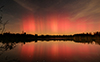 |
Figure 1 Red aurora on 24 September 2023 at 23 UT (or in term of local time, September 25 at 1 LT) at 48.3° geographic north and 1.2° geographic east (49.88°N, 84.55°E in geomagnetic coordinates). The pointing direction is North = North-West, as seen from the Ursa Major constellation. The bottom of the red emission is at an elevation of about 5° and its top at an elevation of about 25°. |
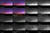 |
Figure 2 Blue and red aurora on 25 September 2023 at 2 UT (4 LT), same location as in Figure 1. The upper left four panels are the succession of frames during 12 mn duration. The different RGB channels are given on the four upper right panels (red), lower left (Green) and lower right (Blue). |
With a single observation, it is not possible to determine whether the blue component is above the red one, behind or in front of it. In this Figure 2, we show a series of four frames at 2 h 6 mn UT, 2 h 12 mn UT, 2 h 15 mn UT and 2 h 18 mn UT. The full time-lapse video is provided in Supplementary material. We also show the different colour channels for each image, as Red-Green-Blue (RGB) decomposition. Here again, the green line is invisible and only red and blue show up. In the following, we discuss all these features in detail.
The current observation benefited from a clear sky while all the higher latitudes were covered with clouds, preventing simultaneous observations below the aurora itself. A geomagnetic storm was under way at the same time with effects down to middle latitudes. Figure 3 shows different Solar wind parameters (Papitashvili & King, 2020) and Hp30 (Matzka et al., 2021). The interplanetary magnetic field z component reverses between northward and southward directions several times within a 7-hour interval. The solar wind velocity is moderate at about 460 km · s−1 but the solar wind density increases to more than 30 cm−3. Hp30 reaches occasionally the value of 6 during the time of the current observations. In term of DST (not shown here), this event corresponds to a weak magnetic storm with a value down to −64 nT. To our knowledge, no other ground instrument was available. In particular, the SuperDarn network cannot provide ionospheric parameters down to such low latitudes. The IMF turned northward at 4 UT (6 LT) and changed from North to South during the period of the blue aurora observation. Unfortunately, no spacecraft measured the precipitation above this phenomenon at the same time. The Cluster II magnetic footprint projection is at Icelandic level (Robert & Dunlop, 2022 and references herein). The closest DMSP passage is F18 (over eastern Germany, northern Italy and Corsica) and too late, around 03:45 UT. Although the ESA Swarm satellite constellation has no precipitating particle detector, it has a Langmuir probe (Pakhotin et al., 2022) which could provide a qualitative indication of the upper atmosphere state through the electron temperature. However, the closest passage to France (also over Germany) was on 25 September at around 15 UT, so too late as well.
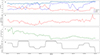 |
Figure 3 Geomagnetic and solar data before, during and after the event described in this paper. X-axis: UT. From top to bottom: (a) Interplanetary magnetic field near Sun-Earth L1 [nT]. The blue diamond line represents the total magnetic field. The red is the y component, the blue line is the z component. (b) Solar wind velocity near L1 [km · s−1]. (c) Solar wind density at L1 [cm−3]. (d) Hp30 index. |
Artificial lights are visible on the series of photographs displayed in Figure 2. One way of showing the temporal dynamics of light phenomena is to subtract two images taken at a given time interval. The result is an image in which any static light over the time interval, such as light pollution, is eliminated. Moreover, any variation in the brightness of the phenomenon over the time interval in question – increase or decrease in overall brightness – will result in an increased light intensity in the final image. The stronger the variation in luminosity during the time interval, the stronger the luminosity in the resulting image. We show such subtractions carried out over four successive time intervals, in the red channel (Fig. 4), the blue channel (Fig. 5) and in both colours simultaneously (Fig. 6). The dynamics revealed by these subtractions rule out any link between the observed phenomenon and light pollution, which is fixed in nature. The movement of clouds remains clearly visible in the red channel, as they reflect light pollution emitted from the ground – mainly sodium lamps – while moving. Firstly, we can observe that blue intensity variations are generally higher on the horizon than red ones. Secondly, blue and red intensity variations are not observed systematically at the same place simultaneously. Interestingly, for these subtractions, and in contrast to the original images, no processing was applied to the blue layer. This implies that brightness variations in the blue channel can be of the same order of magnitude as those in the red channel.
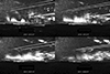 |
Figure 4 Differences between frames taken 3–4 min apart in the red channel. Bright diffuse veils are variation in intensity in the red aurora, while compact structures and straight lines are clouds and contrails, respectively. |
 |
Figure 5 Differences between frames taken 3–4 min apart in the blue channel. Bright blobs and pillars are variation in intensity in the blue aurora (clouds and contrails are barely visible in the blue channel. |
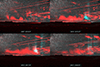 |
Figure 6 Merging of the two previous figures: Differences between frames taken a few minutes apart in both red and blue channels. This makes it possible to see whether or not changes are taking place in the same places, for both colours. |
2.1 Observation equipment
The camera is a canon 6D is partially unfiltered. Usual cameras are filtered in order to follow the human eye sensitivity. Fully suppressing the filter is not possible, but a partial unfiltering allows increasing the signal-to-noise ratio for the red channel, to be more sensitive to the Hα emission line. It was equipped with a Sigma 20-mm focal length lens, opened at F/2.2. It was installed horizontally so that the horizon is at +0° with a field of view from +40° (top of the picture) down to −20°. The optical system was characterized at the Belgian Radiometric Characterization Laboratory (B.RCLab) located in Brussels, in the laboratories of the Royal Institute for Space Aeronomy of Belgium (BIRA-IASB). The Canon 6D and its lens were placed in front of an integrating sphere, which was illuminated at a desired wavelength with a 1-nm full width at half maximum (FWHM) spectral resolution, using one white lamp source and a Bentham double monochromator. A reference silicon (Si) photodiode, wavelength-calibrated by the Physikalisch-Technische Bundesanstalt (PTB) in spectral power responsivity (A/W), from 200 nm to 1100 nm was also measuring the signal from the integrating sphere to obtain the actual power coming from the lamp. However, the integrating sphere is not big enough to insure a proper homogeneous flat-field for the full frame camera. We then can only provide some relative intensities regarding the RBG response. The normalised response of the Canon 6D detector for the spectral range 400–715 nm in the center of the camera sensor is shown in Figure 7.
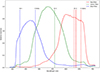 |
Figure 7 Relative intensity response of the camera in the center of the camera sensor as a function of wavelength in the three RGB channels. The wavelengths of the main auroral lines are also displayed. |
3 Interpretation
3.1 Determining the latitude and altitude of the aurora
With a simple series of frames, it is impossible to precisely locate geographically this aurora. The ideal way would be triangulation. This was not possible in our case in spite of numerous searches for alternative frames in other remote places. The first difficulty is that most of northern Europe was covered with clouds. The second difficulty is that we are dealing with a diffuse aurora. This makes it impossible to use triangulation techniques as no individual structure in the aurora can be identified as a common feature seen from different observing points. The exact coordination time is also a strong difficulty. Finally, a triangulation necessitates insuring a wavelength-calibrated white balance of the camera and a good reference point in the picture. For all these reasons, the authors have so far failed to locate the aurora with this method. However, the case is not totally desperate. The ovation prime model1 estimated the location of the auroral oval for September 25 at 2 UTC. This model is mainly used for predicting visible aurora (Machol et al., 2012; Newell et al., 2014), and, in the present case, is good enough to estimate where the oval was in relation to the observer. It shows a strong enhancement of the precipitation at a latitude around 65°–70° geographic north and a longitude of 15° geographic east, above the north part of Norway, as can be seen in Figure 8.
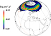 |
Figure 8 Computation of the auroral oval location from the Ovation code (see text), (Newell et al., 2014). This figure stands for the conditions prevailing during the current blue aurora observation. |
Using this model output, we can estimate an upper limit for the altitude of the lower border of the aurora. Geometry computations described in Appendix A show that, from the point of view of the observer at geographic 48.3° N, 1.2° E, the aurora will be seen from 337 km altitude and upwards if it takes place at geographic 65° N and from 535 km altitude and upwards if it takes place at geographic 70°N. Its azimuth of 18° and 12° also agrees with the observations. An aurora is usually fainter at such altitudes and therefore, it would require being quite bright to be observed. In the next subsections, we will analyze whether or not an electron aurora could emit blue at high altitude without emitting in the red/green, then analyze if a proton aurora could be responsible for the emissions, and finally evaluate the scattering of UV light by  at 427.8 nm.
3.2 Aurora due to direct local electron precipitation
The flux of electron precipitation (cm−2 · s−1) is the main source of polar lights. It is out of the scope of this study to review all the efforts that have been developed over the last century to study the auroral spectrum. It is sufficient to remark that the characterisation of the auroral spectrum relies on thousands of spectroscopic measurements. A first review of the efforts up to the 1970s may be found in (Gattinger & Jones, 1974). The same authors recently updated these observations, running more sophisticated instruments (Gattinger et al., 2010). In parallel to field observations, several numerical models have been developed over the last 50 years that have proven to be efficient in reproducing these polar emissions through electron precipitation impact on the upper atmosphere.
They all solve the kinetic Boltzmann transport equation either through a Monte-Carlo (Solomon, 2001) or a physics-based approach (Solomon, 2001; Lilensten et al., 2015). A comparison of the different techniques may be found in Grubbs et al. (2018). To summarize, the main features in the auroral spectrum through electron precipitation are:
The main emission is the green line at 557.7 nm due to the de-excitation of the atomic oxygen from the O(1S) state to the O(1D) state. The altitude of this peak emission is about 110 km on average. Different processes are at the origin of this line, including complex de-excitation of excited N2 (Gronoff et al., 2008).
At higher altitude (typically 220 km), the de-excitation of the O(1D) state to the ground state O(3P) results in the red line at 630 nm (actually, a triplet). The bottom layer of the red line emission is typically about 170 km. The green and red line dayglow emissions were fully modelled in Witasse et al. (1999).
At lower altitude, typically around 85 km, the spectrum is dominated by the ionized molecular nitrogen first negative band  with two main emissions: the purple one at 391.4 nm and the blue one at 427.8 nm. Since the blue line emission is excited by electron impact only, its intensity is directly proportional to the energy flux of electrons at the top of the atmosphere. A thorough review of the different molecular Nitrogen emissions (neutral or ionized) may be found in Lofthus & Krupenie (1977).
The auroral spectrum is of course much more complex than these four emissions but these four are the only ones that can be pictured by a commercial camera in the case of electron precipitation aurorae (Hα and Hβ will be discussed in the Sect. 3.3). They are sufficient for discussing the observation made on 25 September 2023. From the geometry provided in Appendix A and considering that the bottom of this red aurora (taken as 170 km) is at an elevation of about +3°, the E region is almost fully hidden by the Earth (below 107 km) so that most of the green line and any nitrogen lines are invisible and under the horizon. Moreover, the green colours are scattered more efficiently by the atmosphere, so that the possible part where the green emission takes place cannot be seen. With these considerations, the latitude of this aurora is expected to be about geographic 58°N. This behaviour is radically different from that of the event taking place at 4 LT (2 UT).
There are one or two layers with the red and the blue emissions sometimes merged, and sometimes apparently distinct.
The timelapse video2 and the images subtractions shown in Figure 6 suggest that the in some occasions, features such as auroral arcs or pillars occur at the same time in the red and blue channels. This is an indication that when this occurs, the two happen in the same vertical plane.
Most of the time, the blue emission seems to happen above the red emission. However, on several occasions, they are difficult to separate, as both take place at the same altitude and location.
If the blue aurora is from the nitrogen first negative band, we can assume that it is emitted at about 95 km where N2 is most abundant. Taking the lowest elevation of blue aurora in Figure 2 to be at about 1°, we can estimate that the geographic latitude of the aurora would be about 57°. The green line emission should be visible at around 110 km altitude. However, there is no green aurora observed.
For all these reasons, the hypothesis of an aurora due to electron precipitation in the E region must be ruled out.
3.3 Proton aurora
Let us now examine a second assumption, that of a proton aurora. It is out of scope of this study to detail all the findings done around such aurorae since their discovery by Vegard (1939). A recent review is highly recommended, that of Gallardo-Lacourt et al. (2021) which deals particularly with their optical emissions in the subauroral region. A proton aurora arises when incident keV protons collide and charge exchange with the ambient plasma, with the resulting neutral hydrogen radiating in the Balmer series. In order to penetrate the upper atmosphere, their pitch angle (the angle between their trajectory and the local magnetic field line) must be of the order of few degrees. Two Balmer emission lines are usually observed, the Hβ line at 486.1 nm (blue) and the Hα line at 656.3 nm (red). The ratio between the two depends on the precipitated energy.
In Figure 9, we show such an auroral spectrum measured by the “Auroral Spectrograph in Skibotn” (ASIS) instrument on 5 November 2023. Since October 2023, ASIS has been permanently installed at the Skibotn Observatory in Norway to regularly monitor the auroral spectrum between 400 and 700 nm.
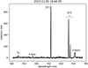 |
Figure 9 Observed spectrum during a proton event as measured by the ASIS instrument from Skibotn, Norway. |
Proton aurora can take place along with an electron aurora, but isolated proton aurorae (sometimes referred to as IPAs) have already been identified and characterized (Frey et al., 2004). They are linked to the ring current. They are produced in the F-region and associated to field-aligned currents produced by electromagnetic ion cyclotron Pc1 waves (Kim et al., 2021). Zhou et al. (2021) observed a detached proton arc at subauroral latitudes using observations of the Special Sensor Ultraviolet Spectrographic Imager on board the Defense Meteorological Satellite Program (DMSP) spacecraft. They showed that the subauroral proton arc was detached and moved dynamically from the auroral oval toward the equator.
The transport of protons in the upper atmosphere is described by a series of coupled kinetic Boltzmann equations, one for H and one for H+. These equations have been solved by Galand et al. (1997, 1998); Lilensten and Galand (1998). The resulting code was fully updated in Simon-Wedlund et al. (2007) where it was coupled with an electron transport code. The two coupled transport models were adapted to any planetary atmosphere in Gronoff et al. (2009, 2012a,b). We ran this code in the current conditions of observations with different precipitating conditions. In Figure 10, we show one example amongst the series of runs, since all exhibit the same behaviour. The two emissions peak at the same altitude, between 110 km and 140 km. With these altitudes and, considering Figure 2, the aurora is expected to be produced at a North geographic latitude between 50.5° and 53.8°. The solar zenith angle at this location is almost 110°.
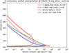 |
Figure 10 Production of the Balmer Hβ (blue line) and Hα (dashed red) emissions due to proton precipitation. For the sake of clarity, we choose a vertical Dirac distribution as the proton energy spectrum at 10 keV. The total energy is 5 erg. The green and red emissions of atomic oxygen are also shown, in their respective colour, to highlight that proton precipitation will lead to these emissions being the most important above 180 km altitude. Therefore, these cannot explain the current observation of blue emissions only. |
We can make several statements in order to confirm or exclude the proton precipitation as the cause of the current observation.
As already mentioned, the Hβ line at 486 nm should appear in both green and blue channels of the camera. Should it be present in the observations, it would create a clear signal in the difference between successive frames in both. However, such a difference exists in the blue range of the camera (Fig. 5) but no difference shows up in the green range (not shown here).
The two emissions should be produced at the same altitude. On the time-lapse video (provided as Supplementary material) or in Figure 2, one sees a series of layers. The blue seems more intense at higher altitude, merged with the red below and finally the red looks isolated at the bottom of the photographs. This could be an indication that the cause is not a proton aurora. However, the light pollution is severe at the lower altitude and saturates the red: the lowermost colour is then very probably due to the light pollution.
Any time the Balmer lines are excited, there is a strong emission of the atomic oxygen at 630 nm (red, around 220 km height) and 577.7 nm (green around 110 km). These are not seen on the current observation. This is not compatible with a proton aurora since the green emission should also appear as seen in Figure 10.
Should the proton aurora assumption be correct, it would be difficult to explain why the blue seems so intense at the higher altitudes, while the modelling shows that it should be an order of magnitude smaller than the Hβ and than the green line.
This series of statements seems to rule out the proton assumption. In addition, it shows that a proton aurora at Earth cannot appear only blue, but will be mixed with green and red.
3.4 Mixture of molecular nitrogen emissions
Another interpretation could be the addition of different N2 emissions. In the blue range, we find the Vegard Kaplan (VK), and the 2nd positive bands. The VK band emits from 180 to 500 nm, but is intense in the blue part (380–450 nm). The second positive is emitting in the blue band around 400 to 500 nm. Apart from the purple 1st line of  , this ion also emits at 427 nm, i.e. in the blue range. N2 also emits in the red range, especially through the 1st positive band, mainly between 600 and 700 nm (see e.g. Schunk & Nagy (2009) and references herein).
We performed a simulation using a kinetic electron transport code that has been developed by several of the authors of this paper since 1994 (Lummerzheim & Lilensten, 1994) and constantly improved and upgraded since then (Marif & Lilensten, 2020; Bouziane et al., 2022). The C++ version ran here is called Aeroplanets and includes several improvements (Gronoff et al., 2008). From an electron (or proton) precipitation flux (in, e.g., cm−2 · s−1 · eV−1 · sr−1), Aeroplanets is able to compute the electron flux at each altitude of an ionosphere by computing the particle transport (Gronoff et al., 2012a,b; Hughes et al., 2023).
The excitation rates are deduced from this flux from which the de-excitation is a straightforward product. The updated collision cross-sections come from the ATMOCIAD database (version 2) Gronoff et al. (2025). For the VK, we used the work of Degen (1982) to assess the fraction that is emitted between 410 and 480 nm, which corresponds to the range where the camera detector is sensitive to the blue channel without being too sensitive to the green channel. This corresponds to 10% of the total Vegard-Kaplan emission.
In Figure 11, we show the result of this simulation at the same location of the observation, i.e. mid-latitude. The initial conditions are electron precipitation, with a mean energy of 5 keV and a total energy of 5 ergs. These values are only chosen for coherency with the proton simulation above (Sect. 3.3) and are very probably far from the real conditions on that night. However, this simulation helps determine the altitude of these emissions and their relative intensity. The  blue emission is small compared to the second positive band and can be neglected. In that case, only emissions due to the excitation of neutral N2 can be considered. The effect of the VK emission is mainly to uplift the total blue emission above the red one, with a peak altitude of about 122 km for the former and 118 for the later. The red and blue emissions have quite similar intensities. The fact that there is no visible green emission can be due to a position of this aurora above Northern UK, hiding this lower layer. Interestingly, the excitation thresholds are lower than that of
  . NN2 which allows understanding why there is no purple emission. N2 is also the most abundant component of the lower thermosphere and there is no problem with this source. Finally, we see a superposition of the blue slightly above the red emission.
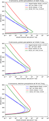 |
Figure 11 Vegard-Kaplan and |

However, this mechanism requires a huge amount of low energy electrons with no high-energy electrons at low altitude. Such electrons can be created on the dayside and transported to the nightside through electrodynamics (Kelley & Miller, 1997) but this mechanism is hardly assessed in the literature and we have no means to check this assumption in the current observation. Moreover, low energy precipitation is stopped above the E region (Rees, 1989). Finally, it is not possible with that process to get blue aurorae without green and red aurorae. In the current situation, it means that these auroral emissions cannot account for the observations and we need to find another process to explain the observations.
3.5 The resonant scattering hypothesis
The resonant scattering was first observed by Störmer (1938) and its mechanism was proposed by Bates & Seaton (1949). It was fully studied by Broadfoot (1967). It is the following: when the molecular nitrogen ions are illuminated by the Sun above the shadow height, it can fluoresce in the blue and violet bands of the first negative system. This mechanism depends on the exospheric temperature, and is therefore enhanced around solar max. That also implies that N2 could be first ionised on the nightside and be further excited when moving into the sunlit region. The mean lifetime for deactivation is the parameter which determines the amount of light emitted through this resonance scattering. Broadfoot (1967) estimates that the resonant scattering enters only for 40% of the total amount of emission due to the first negative band, the remaining part being attributed to direct excitation by the EUV flux.
In order to reconcile the fact that the nitrogen is negligible above typically 200 km, Hunten (2003) focuses on cases when the shadow remains below about 130 km. Since the  ions produced by photoionization can only account for about 40% of first negative band observed emission, they add the contribution of atomic oxygen ionization, which produces some additional
  ions through the charge-exchange reaction:
 (1)
(1)
Finally, Broadfoot & Hunten (1966) propose that an observed winter-evening enhancement of the twilight intensity is due to production of ions by photoelectrons precipitating from the magnetic conjugate point, which is still in daylight. However, this can hardly be the case here since we are very close to equinox. A very comprehensive review of the most recent advances in this field is given in Jokiaho et al. (2009). In this paper, the authors report a statistical study of night-time, twilight and daytime aurora at the solar minimum from the magnetic zenith during 3 months at very high geographic latitude (78° N.), i.e. in very different conditions from the current observation, they find a maximum altitude of 260 km for the 1NG band through resonant scattering. Above 300 km, the emission brightness is divided by about 4. Their main result is that for shadow heights above about 400 km, the 1 NG bands and their ratios are almost unaffected, but for shadow heights below 150 km (i.e. fully illuminated), there are significant enhancements that increase with decreasing energy.
Shiokawa et al. (2019) study the 427.8 nm emission caused by precipitation of energetic electrons or by resonant scattering of sunlight at subauroral latitudes, i.e. a magnetic latitude of 62° over 14 years. From this study, the occurrence rate of resonant scattering is high in the postmidnight sector and depends on the geomagnetic activity. The occurrence rate is lowest in winter. In order to perform this study, they consider a threshold at a solar zenith angle of 114°: any situation with a solar zenith angle larger than 114° is under the dark (no sunlight) condition.
Ellingsen et al. (2021) present measurements of sunlit aurora during the launch of a Rocket Experiment for Neutral Upwelling in December 2015, coinciding with sunlit aurora. They use a meridian-scanning photometer to measure the coordinated 391.4 and 427.8 nm  emissions and show that the sunlit aurora constitutes about 40% of the observed 427.8 nm emission. The authors mention that if the upwelling of neutrals and ions is known to take place in the cusp region of the auroral oval, the underlying mechanisms are not fully understood. Although these observations are performed above the Svalbard archipelago, i.e. at polar latitudes, this conclusion is very important and casts some light on our own observations, despite the fact that, in their case, the blue 427.8 nm emission is produced at the same altitude as the red 630 nm one, which is not systematically the case in our observation. Romick et al. (1999) also show satellite observation of the resonant aurora over the polar cap up to 900 km altitude. These authors mention that the mechanism involved is ion upflow.
The resonant scattering has therefore already been observed and its existence can hardly be questioned. It raises the very interesting question of how to lift up enough  to generate the blue emission seen from the ground. There are two ways. The first one is to lift up the E-region neutral molecular nitrogen that will be ionized at higher altitude, either by precipitating electrons or by the solar EUV flux. This necessitates a very strong molecular diffusion. Such a diffusion is however not efficient in the lower E region where N2 is most abundant because it is overcome by the collisions and the eddy diffusion (Lilensten & Blelly, 2000). However, gravity waves and their ionospheric signature designated as travelling ionospheric disturbances (Prösll, 2004; Kaladze et al., 2008) can still be the reason for the uplift (Karpov & Kshevetskii, 2017). In that case, not only N2 but also O2 may rise up. Gravity waves take place during perturbed periods, which is the case in the current situation (see the review in Nishimura et al. (2022, Chapter 7).
The second way is to lift up the already E-region ionized nitrogen  . Here, the mechanism is the ambipolar diffusion. In order to be efficient, the gradient of the plasma temperature
  where the subscript e stands for electrons, i for ions, p for plasma, must be high. That is perfectly possible in the current perturbed conditions. The most efficient mechanism to heat the ions above the electron temperature is the electric field. Electric fields parallel to the magnetic field are the best configuration to also lift the ions up.
Let us consider the current geometry, if we take the altitude of 350 km at geographic 65°N and we compute the line of sight to the Sun at 02:00 UTC, we see that it is tangent to the Earth at an altitude of 40 km, therefore the sunlight in 300–500 nm region is not strongly absorbed and is able to be diffused by  .
.
Similarly, at geographic 70°N and 550 km altitude, the tangent altitude of the line of sight to the Sun is 338 km, which means that there is no absorption in the blue. These computations show that a scattering of the blue light from the Sun at these altitudes is a possible emission mechanism.
We can make several statements in order to assess the resonant scattering mechanism as the cause of the current observation.
The resonant scattering accounts for up to 40% of the total 1N band system intensity (Hunten, 2003; Jokiaho et al., 2009). It requires that the existing
 at ground level (state
  that exists above 340 km is excited with a blue emission (427.8 nm) up to the
  state. This state radiates the same emission over a 4π sphere, is absorbed again so that resonant scattering takes place from an
  molecule at ground level to a neighbouring
  molecule at ground level. In the current configuration with a solar zenith angle of 108.4°, the sunlight already crossed the ionosphere on the dayside, continued in the troposphere before crossing the different upper layers (strato sphere, mesosphere, thermosphere) again in order to illuminate the upper atmosphere above the observation. However, it is difficult to assess whether the blue part of the solar spectrum has been absorbed from the dayside to the point of observation (see e.g. Hobbs, 2012). We therefore cannot rule out the resonant scattering based on this consideration.
The remaining 60% of the total 1NG band system intensity are usually due to direct ionization by the solar EUV flux (Broadfoot, 1967). The energy threshold to create
 at ground level (state
  ) is 15.58 eV or, in terms of electromagnetic wave, a wavelength of 79.59 nm. Two states are mainly excited, A2Πu and
  with respective thresholds of 16.73 (74.12 nm) and 18.75 eV (66.13 nm). The branching ratios of these three states are 0.48, 0.45 and 0.07, respectively, for precipitated electrons above the highest energy threshold or EUV emissions below 66.13 nm (many textbook refer to these values. See e.g. Rees, 1989). In the current configuration, all the EUV flux is absorbed on the dayside (by ionisation and excitation of the ambient thermosphere) (Rees, 1989; Lilensten et al., 2007). There is therefore no energy left to ionize N2 in any state.
From the pictures (Fig. 2), the blue emission is seen at an elevation of about 20°. With such an elevation, the altitude above which the aurora is illuminated by the Sun is 340 km. The latitude of the aurora is then geographic 55.4°N where the solar zenith angle is 108.4°. This value is quite close to the 114° threshold in (Shiokawa et al., 2019). With these parameters, the E region is fully visible.
Since the observation is made close to the equinox, the conjugated point in the southern hemi sphere is also in the night. There is therefore no direct photoionisation that could produce high energy electrons in the southern hemisphere able to precipitate in the northern hemisphere to create
 .
. 1NG could also be created at higher latitudes by electron precipitation and be transported upwards by parallel electric fields. The inclination of the magnetic field is 63.37° at 400 km altitude. Following the magnetic field lines, the
  would then be created quite close to the observation point, at a latitude of about geographic 48.45°N. At such a short distance (about 102 km), the E region is perfectly visible and one should see the presence of a strong green emission, since the O(1S) state is always excited when the
  is.
is.-
We finally ran the International Reference Ionosphere (IRI) (Bilitza & Reinisch, 2021). For given location, time and date, IRI provides monthly averages of the electron density, electron temperature, ion temperature, and ion composition in the ionospheric altitude range, for the conditions prevailing during these observations. The major ion up to 600 km height is O+. The model foresees no
 at all. Of course, and even using the switches provided in IRI, this is only a model. In particular, it does not take into account vertical diffusion processes in highly disturbed environments. This prevents an easy estimation of the
  density for these models and require dedicated polar wind models. The ion profiles are shown in Figure 12.
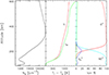
Figure 12 Ionospheric profiles forecasts by the IRI ionospheric model for the conditions prevailing during the observation. Left panel: Electron density. Middle panel: Ion temperature (red line) and electron temperature (green line). Right panel: ion rates. Red line: O+; Light blue: NO+; dark blue:
 . The other ions (N+ and H+) are shown but negligible.
To summarize: to have a sunlit aurora, we need to have  lifted (or produced) in regions lit by the Sun, however, modeling shows that the direct photoionization is not enough to provide the sufficient amount of ions for explaining the aurora Jokiaho et al. (2009). It is therefore necessary to have electron precipitations of the order of the hundreds of electron Volts to keV to create the
  and the conditions for its lift-up above 300 km Jokiaho et al. (2009). Since precipitating electrons allow the type 2 ion outflow of
  , we still have enough electrons at the location of the up-flow to obtain an optical aurora. Therefore, the sunlit aurora will typically be above the standard optical aurora; hence, trying to locate the green/red aurora will help us checking if it is likely that the blue aurora could be due to the sunlit. Since we do not have a second camera to triangulate the aurora, we need to use other methods to try to find the most likely place of the aurora. In the present case, OVATION (Fig. 8) and the observations from Aurorasaurus MacDonald et al. (2015) (some user in Northern England and Scotland were able to observe the green aurora on the Northern horizon) are our only other sources: following those, the location of the optical aurora and therefore the most likely location of the blue aurora is at a place where it could be sunlit and observed from our mid-latitude location.
The discussion above shows that the resonant scattering cannot be ruled out as a candidate to explain the observed blue aurora. It raises several questions that must be solved in the future to ascertain this mechanism as the main cause. It remains the most likely candidate to explain the observations.
4 Conclusion
A single blue aurora has been observed at a mid-latitude site in September 2023. At the present state of scientific knowledge such phenomenon are unpredictable. This makes it impossible to dedicate many nights of operating scientific instrumentation to this endeavor. Analyzing the current observations of the September 25, 2023 blue aurora left one mechanism as the most likely cause, that is, the resonant scattering of the  ions at high altitude. Other mechanisms such as electron or proton precipitation appear much more unlikely. Most of the
  is first created in the E-region. However, in this case, it is not leading directly to the aurora visible in the images (even though there is likely a green aurora below the blue one, but not visible from the location where the pictures are taken because they are below the horizon). The produced
  is expected to be subsequently uplifted by ambipolar diffusion and undergo resonant scattering in the upper F-region.
While this article was submitted, a parallel work was submitted to another journal (Nanjo & Shiokawa, 2024). In this article, the authors refer to the Mother’s day event in May 2024, as seen from Japan. They too observe a blue aurora but could use the observations of two astrophotographers, allowing a more precise determination of the location and altitude of the aurora than ours. They observe a blue-dominant aurora likely including emissions at 427.8 nm up to 900 km. They suggest that these emissions are due to energetic neutral atoms from the ring current but propose alternative explanations. These two articles, published simultaneously, show that this topic is still not understood fully and deserves some attention.
In order to progress in the understanding of these aurorae, science can only rely on astrophotographers. The amateur community can provide an incredible manpower, and knows how to analyze their cameras, as this contribution shows. Good examples of such observations can be found on the SpaceWeatherLive website3. In the same spirit, a large effort has started in order to better characterize the later Mother Day event (or Gannon in other naming) that occurred 10 May, 2024 (Grandin et al., 2024). Here, 696 citizen science reports from over 30 countries could be gathered. We therefore recommend to join the (Grandin et al., 2024) initiative – or any other one in order to explore this still little-known kind of aurora, gathering amateurs and professionals.
Acknowledgments
We thank the Institut de Physique du Globe for supporting its operation and INTERMAGNET for insuring high standards of magnetic observatory practice (https://www.intermagnet.org). We thank the Action Nationale Soleil Terre (ATST) for supporting this research. We acknowledge the Community Coordinated Modeling Center (CCMC) at Goddard Space Flight Center for the use of the Ovation-Prime model results. OVATION Prime was developed at Johns Hopkins Applied Physics Laboratory (JHU-APL) by Patrick Newell and co-workers. It can be accessed at https://ccmc.gsfc.nasa.gov/models/Ovation-Prime~2.3. The editor thanks two anonymous reviewers for their assistance in evaluating this paper.
Funding
JL’s fundings for this research has been provided by ATST, the French national program for solar terrestrial physics. GG’s funding was provided by the ROSES Solar System Working program(Grant 80NSSC20K0317) and the NASA Science Mission Directorate, Heliophysics Division, Space Weather Science Applications Program. CSW thanks the Austrian Science Fund (FWF) for funding through the Project 10.55776/P35954.
Conflicts of interest
There is no conflict of interest from any of the authors with any of the topics in this paper.
Data availability statement
All data are freely available upon request to the authors.
Author contributions statement
All authors participated in the scientific discussions. EB made the observations and took the photographs that form the basis of this paper. JL coordinated the group and drafted the manuscript. GC and LB performed the measurements for the spectra of the proton aurorae and performed together with EB the wavelength-calibration of EB’s camera. GG ran the proton transport modelling with the help of CSW. FP performed part of the bibliography. MB suggested the VK/st positive assumption.
Supplementary material
Supplementary file 1: Evolution of the aurora in RGB colors. Exposures of 20 second were taken one after another from 02H05 to 02H22 UT and assembled as a time-lapse. The time-lapse rate is 4 images per second.
Supplementary file 2: Evolution of the aurora in the blue channel. Exposures of 20 second were taken one after another from 02H05 to 02H22 UT and assembled as a time-lapse. The time-lapse rate is 4 images per second.
Supplementary file 3: Evolution of the aurora in the green channel. Exposures of 20 second were taken one after another from 02H05 to 02H22 UT and assembled as a time-lapse. The time-lapse rate is 4 images per second.
Supplementary file 4: Evolution of the aurora in the red channel. Exposures of 20 second were taken one after another from 02H05 to 02H22 UT and assembled as a time-lapse. The time-lapse rate is 4 images per second.
Access Supplementary MaterialAppendix A: The geometry
A.1 Estimation of the altitude of the blue aurora
The geometry of the observation is displayed in Figure A1. The elevation (unknown) of the aurora is noted ϵ, and corresponds to the angle DAC in Figure A1. The altitude of the aurora is then
 (A.1)
(A.1)
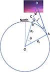 |
Figure A1 Estimation of the altitude of the aurora. O is the center of the Earth, and North is located on the top. The observation is made on A at a latitude latobs and a longitude lonobs. Considering the stars on the pictures, the blue aurora is supposed to happen at the same longitude and a latitude lataur. The line between the aurora and O crosses the surface of the Earth in B. C is the point at the horizon of A, i.e. any point below C is invisible as seen from A. Its altitude of the auora is BD = BC + CD = δ + d. The lenght between A and C is l. RT is the radius of the Earth, i.e. 6370 km. The latitude of the aurora is that of the observer (geographic 48.3°N) plus the angle θ. |
The OAC triangle is rectangle in A, so that
 (A.2)
(A.2)
which yields
 (A.3)
(A.3)
Considering the diameter of the Earth, we also consider the ACD triangle as rectangle in C so that d = AC · tan(ϵ). Equation (A.1) results in a simple second-order equation in AC, from which one easily deduces
 (A.4)
(A.4)
The angle θ is given by
 (A.5)
(A.5)
The horizon altitude δ is deduced from equation (A.3). It can also be obtained from
 (A.6)
(A.6)
Both give similar results. Therefore, the latitude of the aurora can only be estimated by assuming different values for its elevation (as seen from the camera) and for its actual altitude.
A.2 Estimation of the altitude illuminated by the Sun
Calculating the altitude illuminated by the Sun is straightforward and is presented in Figure A2. From the figure, the altitude hSun at which the Sun is visible is simply
 (8)
(8)
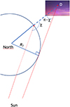 |
Figure A2 Estimation of the altitude illuminated by the Sun. This figure represents the Earth as seen from above the North pole. χ is the solar zenith angle. RT is the radius of the Earth. |
The solar zenith angle is classically computed from
 (9)
(9)
where δ is the declination of the Sun equal to  , and ϕ is the latitude of the potential aurora.
Visible at adress.swsc.tobeprovidedbySWSC.fr.
References
- Bates DR, Seaton MJ. 1949. The quantal theory of continuous absorption of radiation by various atoms in their ground states. II. Further calculations on oxygen, nitrogen and carbon. Mon Not R Astron Soc 109: 698. https://doi.org/10.1093/mnras/109.6.698. [CrossRef] [Google Scholar]
- Bilitza D, Reinisch BW. 2021. Preface: international reference ionosphere – progress and new inputs. Adv Space Res 68(5): 2057–2058. https://doi.org/10.1016/j.asr.2021.04.015. [CrossRef] [Google Scholar]
- Bouziane A, Amin Ferdi M, Djebli M. 2022. Studying nighttime nitric oxide emission at 5.3 μm during the geomagnetic storm in the Earth’s ionosphere. Astrophys Space Sci 367: 3. https://doi.org/10.1007/s10509-021-04037-y. [CrossRef] [Google Scholar]
-
Broadfoot AL. 1967. Resonance scattering by
 . Planet Space Sci 15(12): 1801–1815. https://doi.org/10.1016/0032-0633(67)90017-7.
[CrossRef]
[Google Scholar]
. Planet Space Sci 15(12): 1801–1815. https://doi.org/10.1016/0032-0633(67)90017-7.
[CrossRef]
[Google Scholar]
-
Broadfoot AL, Hunten DM. 1966.
 emission in the twilight. Planet Space Sci 14(12): 1303–1319. https://doi.org/10.1016/0032-0633(66)90083-3.
[CrossRef]
[Google Scholar]
emission in the twilight. Planet Space Sci 14(12): 1303–1319. https://doi.org/10.1016/0032-0633(66)90083-3.
[CrossRef]
[Google Scholar]
- Degen V. 1982. Synthetic spectra for auroral studies: The N2 Vegard-Kaplan band system. J Geophys Res 87(A12): 10541–10547. https://doi.org/10.1029/JA087iA12p10541. [CrossRef] [Google Scholar]
- Egeland A, Burke WJ. 2019. Auroral hydrogen emissions: a historic survey. Hist Geo- Space Sci 10(1): 201–213. https://doi.org/10.5194/hgss-10-201-2019. [CrossRef] [Google Scholar]
-
Ellingsen PG, Lorentzen D, Kenward D, Hecht JH, Evans JS, Sigernes F, Lessard M. 2021. Observations of sunlit
 aurora at high altitudes during the RENU2 flight. Ann Geophys 39(5): 849–859. https://doi.org/10.5194/angeo-39-849-2021.
[CrossRef]
[Google Scholar]
aurora at high altitudes during the RENU2 flight. Ann Geophys 39(5): 849–859. https://doi.org/10.5194/angeo-39-849-2021.
[CrossRef]
[Google Scholar]
- Feldman PD, Doering JP. 1975. Auroral electrons and the optical emissions of nitrogen. J Geophys Res 80(19): 2808–2812. https://doi.org/10.1029/JA080i019p02808. [CrossRef] [Google Scholar]
- Frey HU, Haerendel G, Mende SB, Forrester WT, Immel TJ, ØStgaard N. 2004. Subauroral morning proton spots (SAMPS) as a result of plasmapause-ring-current interaction. J Geophys Res Space Phy 109(A10): A10305. https://doi.org/10.1029/2004JA010516. [Google Scholar]
- Galand M, Lilensten J, Kofman W, Lummerzheim D. 1998. Proton transport model in the ionosphere. 2. Influence of magnetic mirroring and collisions on the angular redistribution in a proton beam. Ann Geophys 16(10): 1308–1321. https://doi.org/10.1007/s00585-998-1308-y. [CrossRef] [Google Scholar]
- Galand M, Lilensten J, Kofman W, Sidje RB. 1997. Proton transport model in the ionosphere 1. Multistream approach of the transport equations. J Geophys Res 102(10): 22261–22272. https://doi.org/10.1029/97JA01903. [CrossRef] [Google Scholar]
- Gallardo-Lacourt B, Frey HU, Martinis C. 2021. Proton aurora and optical emissions in the subauroral region. Space Sci Rev 217(1): 10. https://doi.org/10.1007/s11214-020-00776-6. [CrossRef] [Google Scholar]
- Gattinger RL, Jones AV. 1974. Quantitative spectroscopy of the aurora II – the spectrum of medium intensity aurora between 4500 and 8900 A. Can J Phys 52: 2343–2356. https://doi.org/10.1139/p74-305. [CrossRef] [Google Scholar]
- Gattinger RL, Vallance Jones A, Degenstein DA, Llewellyn EJ. 2010. Quantitative spectroscopy of the aurora. VI. The auroral spectrum from 275 to 815 nm observed by the OSIRIS spectrograph on board the Odin spacecraft. Can J Phys 88(8): 559–567. https://doi.org/10.1139/P10-037. [CrossRef] [Google Scholar]
- Grandin M, Bruus E, Ledvina VE, Partamies N, Barthelemy M, et al. 2024. The Gannon Storm: citizen science observations during the geomagnetic superstorm of 10 May 2024. Geosci Commun 7(4): 297–316. https://doi.org/10.5194/gc-7-297-2024. [CrossRef] [Google Scholar]
- Gronoff G, Lilensten J, Desorgher L, Flückiger E. 2009. Ionization processes in the atmosphere of Titan. I. Ionization in the whole atmosphere. A&A 506(2): 955–964. https://doi.org/10.1051/0004-6361/200912371. [NASA ADS] [CrossRef] [EDP Sciences] [Google Scholar]
- Gronoff G, Lilensten J, Simon C, Barthélemy M, Leblanc F, Dutuit O. 2008. Modelling the Venusian airglow. A&A 482(3): 1015–1029. https://doi.org/10.1051/0004-6361:20077503. [CrossRef] [EDP Sciences] [Google Scholar]
- Gronoff G, Simon Wedlund C, Mertens CJ, Barthélemy M, Lillis RJ, Witasse O. 2012a. Computing uncertainties in ionosphere-airglow models: II. The Martian airglow. J Geophys Res Space Phys 117(A5): A05309. https://doi.org/10.1029/2011JA017308. [Google Scholar]
- Gronoff G, Simon Wedlund C, Mertens CJ, Lillis RJ. 2012b. Computing uncertainties in ionosphere-airglow models: I. Electron flux and species production uncertainties for Mars. J Geophys Res Space Phys 117(A4): A04306. https://doi.org/10.1029/2011JA016930. [Google Scholar]
- Gronoff G, Wedlund CS, Hegyi B, Lilensten J, Glocer A, Cessateur G, Witasse O, Mertens CJ. 2025. ATMOCIAD: the atomic and molecular cross-section for ionization and aurora database. Adv Space Res. https://doi.org/10.1016/j.asr.2025.03.061. [Google Scholar]
- Grubbs G, Michell R, Samara M, Hampton D, Hecht J, Solomon S, Jahn J-M. 2018. A Comparative study of spectral auroral intensity predictions from multiple electron transport models. J Geophys Res Space Phys 123(1): 993–1005. https://doi.org/10.1002/2017JA025026. [CrossRef] [Google Scholar]
- Hobbs PV. 2012. Basic physical chemistry for the atmospheric sciences. Cambridge University Press. ISBN 9780511802423. [Google Scholar]
- Hughes ACG, Chaffin M, Mierkiewicz E, Deighan J, Jolitz RD, et al. 2023. Advancing our understanding of martian proton aurora through a coordinated multi-model comparison campaign. J Geophys Res Space Phys 128(10): e2023JA031838. https://doi.org/10.1029/2023JA031838. [CrossRef] [Google Scholar]
-
Hunten DM. 2003. Sunlit aurora and the
 ion: a personal perspective. Planet Space Sci 51(13): 887–890. https://doi.org/10.1016/S0032-0633(03)00079-5.
[CrossRef]
[Google Scholar]
ion: a personal perspective. Planet Space Sci 51(13): 887–890. https://doi.org/10.1016/S0032-0633(03)00079-5.
[CrossRef]
[Google Scholar]
-
Jokiaho O, Lanchester BS, Ivchenko N. 2009. Resonance scattering by auroral
 : steady state theory and observations from Svalbard. Ann Geophys 27(9): 3465–3478. https://doi.org/10.5194/angeo-27-3465-2009.
[CrossRef]
[Google Scholar]
: steady state theory and observations from Svalbard. Ann Geophys 27(9): 3465–3478. https://doi.org/10.5194/angeo-27-3465-2009.
[CrossRef]
[Google Scholar]
- Kaladze TD, Pokhotelov OA, Shah HA, Khan MI, Stenflo L. 2008. Acoustic-gravity waves in the Earth’s ionosphere. J Atmos Sol Terr Phys 70(13): 1607–1616. https://doi.org/10.1016/j.jastp.2008.06.009. [CrossRef] [Google Scholar]
- Kaplan J. 1935. Light of the night sky. Planet Space Sci 47(279): 257. https://doi.org/10.1086/124605. [Google Scholar]
- Karpov IV, Kshevetskii SP. 2017. Numerical study of heating the upper atmosphere by acoustic-gravity waves from a local source on the Earth’s surface and influence of this heating on the wave propagation conditions. J Atmos Sol Terr Phys 164: 89–96. https://doi.org/10.1016/j.jastp.2017.07.019. [CrossRef] [Google Scholar]
- Kelley MC, Miller CA. 1997. Mid-latitude thermospheric plasma physics and electrodynamics: a review. J Atmos Sol Terr Phys 59: 1643–1654. https://doi.org/10.1016/S1364-6826(96)00163-0. [CrossRef] [Google Scholar]
- Kim H, Shiokawa K, Park J, Miyoshi Y, Miyashita Y, et al.. 2021. Isolated proton aurora driven by EMIC Pc1 Wave: PWING, Swarm, and NOAA POES multi-instrument observations. Geophys Res Lett 48(18): e95090. https://doi.org/10.1029/2021GL095090. [Google Scholar]
- Lilensten J, Blelly P-L. 2000. Du Soleil à la Terre: aéronomie et métérologie de l’espace. EDP Sciences, Paris. [Google Scholar]
- Lilensten J, Bommier V, Barthélemy M, Lamy H, Bernard D, IdarMoen J, Johnsen MG, Løvhaug UP, Pitout F. 2015. The auroral red line polarisation: modelling and measurements. J Space Weather Space Clim 5: A26. https://doi.org/10.1051/swsc/2015027. [CrossRef] [EDP Sciences] [Google Scholar]
- Lilensten J, Dudok de Wit T, Amblard P-O, Aboudarham J, Auchère F, Kretzschmar M. 2007. Recommendation for a set of solar EUV lines to be monitored for aeronomy applications. Ann Geophys 25: 1299–1310. https://doi.org/10.5194/angeo-25-1299-2007. [CrossRef] [Google Scholar]
- Lilensten J, Galand M. 1998. Proton-electron precipitation effects on the electron production and density above EISCAT (Tromsø) and ESR. Ann Geophys 16(10): 1299–1307. https://doi.org/10.1007/s00585-998-1299-8. [CrossRef] [Google Scholar]
- Lofthus A, Krupenie PH. 1977. The spectrum of molecular nitrogen. J Phys Chem Ref Data 6(1): 113–307. https://doi.org/10.1063/1.555546. [CrossRef] [Google Scholar]
- Lummerzheim D, Lilensten J. 1994. Electron transport and energy degradation in the ionosphere: Evaluation of the numerical solution, comparison with laboratory experiments and auroral observations. Ann Geophys 12(10–11): 1039–1051. https://doi.org/10.1007/s00585-994-1039-7. [CrossRef] [Google Scholar]
- MacDonald E, Case N, Clayton J, Hall M, Heavner M, Lalone N, Patel K, Tapia A. 2015. Aurorasaurus: a citizen science platform for viewing and reporting the aurora. Space Weather 13(9): 548–559. https://doi.org/10.1002/2015SW001214. [CrossRef] [Google Scholar]
- Machol JL, Green JC, Redmon RJ, Viereck RA, Newell PT. 2012. Evaluation of OVATION Prime as a forecast model for visible aurorae. Space Weather 10(3): S03005. https://doi.org/10.1029/2011SW000746. [Google Scholar]
- Malville J. 1961. Excitation of helium in the aurora. J Atmos Terr Phys 21(1): 54–64. https://doi.org/10.1016/0021-9169(61)90191-X. [CrossRef] [Google Scholar]
- Marif H, Lilensten J. 2020. Suprathermal electron moments in the ionosphere. J Space Weather Space Clim 10: 22. https://doi.org/10.1051/swsc/2020021. [CrossRef] [EDP Sciences] [Google Scholar]
- Matzka J, Stolle C, Yamazaki Y, Bronkalla O, Morschhauser A. 2021. The geomagnetic Kp index and derived indices of geomagnetic activity. Space Weather 19: e2020SW002641. https://doi.org/10.1029/2020SW002641. [CrossRef] [Google Scholar]
- Megan Gillies D, Knudsen D, Donovan E, Jackel B, Gillies R, Spanswick E. 2017. Identifying the 630 nm auroral arc emission height: A comparison of the triangulation, FAC profile, and electron density methods. J Geophys Res Space Phys 122(8): 8181–8197. https://doi.org/10.1002/2016JA023758. [CrossRef] [Google Scholar]
- Miller JR, Shepherd GG. 1969. Rocket measurements of H beta production in a hydrogen aurora. J Geophys Res 74(21): 4987–4997. https://doi.org/10.1029/JA074i021p04987. [CrossRef] [Google Scholar]
- Nanjo S, Shiokawa K. 2024. Spatial structures of blue low-latitude aurora observed from Japan during the extreme geomagnetic storm of May 2024. Earth Planets Space 76: 156. https://doi.org/10.1186/s40623-024-02090-9. [CrossRef] [Google Scholar]
- Newell PT, Liou K, Zhang Y, Sotirelis T, Paxton LJ, Mitchell EJ. 2014. OVATION Prime – 2013: Extension of auroral precipitation model to higher disturbance levels. Space Weather 12(6): 368–379. https://doi.org/10.1002/2014SW001056. [CrossRef] [Google Scholar]
- Nishimura Y, Verkhoglyadova O, Deng Y, Zhang S-R. 2022. Cross-scale coupling and energy transfer in the magnetosphere-ionosphere-thermosphere system. Elsevier. https://doi.org/10.1016/C2019-0-00526-2. [Google Scholar]
- Papitashvili NE, King JH. 2020. OMNI 5-min ACE [Data set]. NASA Space Physics Data Facility. https://doi.org/10.48322/gbpg-5r77, Accessed on March 26, 2025 [Google Scholar]
- Pakhotin IP, Burchill JK, Förster M, Lomidze L. 2022. The swarm Langmuir probe ion drift, density and effective mass (SLIDEM) product. Earth Planets Space 74(1): 109. https://doi.org/10.1186/s40623-022-01668-5. [CrossRef] [Google Scholar]
- Prösll MH. 2004. Physics of the Earth space environment. Springer. ISBN 3-540-21426-7. [Google Scholar]
- Rees MH. 1989. Physics and chemistry of the upper atmosphere. Cambridge University Press. ISBN 9780511573118. [CrossRef] [Google Scholar]
- Robert P, Dunlop MW. 2022. Use of twenty years CLUSTER/FGM data to observe the mean behavior of the magnetic field and current density of earth’s magnetosphere. J Geophys Res Space Phys 127(1): e29837. https://doi.org/10.1029/2021JA02983710.1002/essoar.10507700.1. [CrossRef] [Google Scholar]
- Romick GJ, Yee JH, Morgan MF, Morrison D, Paxton LJ, Meng CI. 1999. Polar cap optical observations of topside (>900 km) molecular nitrogen ions. Geophys Res Lett 26(7): 1003–1006. https://doi.org/10.1029/1999GL900091. [CrossRef] [Google Scholar]
- Schunk R, Nagy A. 2009. Ionospheres: physics, plasma physics, and chemistry. Cambridge Atmospheric and Space Science Series, Cambridge University Press. https://doi.org/10.1017/CBO9780511635342. [CrossRef] [Google Scholar]
-
Shemansky D, Donahue T, Zipf E. 1972. N2 positive and
 band systems and the energy spectra of auroral electrons. Planet Space Sci 20(6): 905–917. https://doi.org/10.1016/0032-0633(72)90176-6.
[CrossRef]
[Google Scholar]
band systems and the energy spectra of auroral electrons. Planet Space Sci 20(6): 905–917. https://doi.org/10.1016/0032-0633(72)90176-6.
[CrossRef]
[Google Scholar]
- Shiokawa K, Otsuka Y, Connors M. 2019. Statistical study of auroral/resonant-scattering 427.8-nm emission observed at subauroral latitudes over 14 years. J Geophys Res Space Phys 124(11): 9293–9301. https://doi.org/10.1029/2019JA026704. [CrossRef] [Google Scholar]
- Simon-Wedlund C, Lilensten J, Moen J, Holmes JM, Ogawa Y, Oksavik K, Denig WF. 2007. TRANS4: a new coupled electron/proton transport code – comparison to observations above Svalbard using ESR, DMSP and optical measurements. Ann Geophys 25(3): 661–673. https://doi.org/10.5194/angeo-25-661-2007. [CrossRef] [Google Scholar]
- Solomon SC. 2001. Auroral particle transport using Monte Carlo and hybrid methods. J Geophys Res 106(A1): 107–116. https://doi.org/10.1029/2000JA002011. [CrossRef] [Google Scholar]
- Störmer C. 1938. Blue sunlit aurora rays and their spectrum. Nature 142(3606): 1034. https://doi.org/10.1038/1421034a0. [CrossRef] [Google Scholar]
- Vegard L. 1939. Hydrogen showers in the auroral region. Nature 144(3661): 1089–1090. https://doi.org/10.1038/1441089b0. [Google Scholar]
- Witasse O, Lilensten J, Lathuillère C, Blelly PL. 1999. Modeling the OI 630.0 and 557.7 nm ther mospheric dayglow during EISCAT-WINDII coordinated measurements. J Geophys Res 104(A11): 24639–24656. https://doi.org/10.1029/1999JA900260. [CrossRef] [Google Scholar]
- Zhou S, Luan X, Burch JL, Yao Z, Han D-S, Tian C, Chen Y, Zhang J, Yu X, Dai T. 2021. A possible mechanism on the detachment between a subauroral proton arc and the auroral oval. J Geophys Res Space Physics. 126(2): e28493. https://doi.org/10.1029/2020JA028493. [Google Scholar]
Cite this article as: Beaudoin E, Lilensten J, Gronoff G, Cessateur G, Bosse L, et al. 2025. A rare observation from mid-latitude of a blue aurora. J. Space Weather Space Clim. 15, 16. https://doi.org/10.1051/swsc/2025012.
All Figures
|
Figure 1 Red aurora on 24 September 2023 at 23 UT (or in term of local time, September 25 at 1 LT) at 48.3° geographic north and 1.2° geographic east (49.88°N, 84.55°E in geomagnetic coordinates). The pointing direction is North = North-West, as seen from the Ursa Major constellation. The bottom of the red emission is at an elevation of about 5° and its top at an elevation of about 25°. |
| In the text | |
|
Figure 2 Blue and red aurora on 25 September 2023 at 2 UT (4 LT), same location as in Figure 1. The upper left four panels are the succession of frames during 12 mn duration. The different RGB channels are given on the four upper right panels (red), lower left (Green) and lower right (Blue). |
| In the text | |
|
Figure 3 Geomagnetic and solar data before, during and after the event described in this paper. X-axis: UT. From top to bottom: (a) Interplanetary magnetic field near Sun-Earth L1 [nT]. The blue diamond line represents the total magnetic field. The red is the y component, the blue line is the z component. (b) Solar wind velocity near L1 [km · s−1]. (c) Solar wind density at L1 [cm−3]. (d) Hp30 index. |
| In the text | |
|
Figure 4 Differences between frames taken 3–4 min apart in the red channel. Bright diffuse veils are variation in intensity in the red aurora, while compact structures and straight lines are clouds and contrails, respectively. |
| In the text | |
|
Figure 5 Differences between frames taken 3–4 min apart in the blue channel. Bright blobs and pillars are variation in intensity in the blue aurora (clouds and contrails are barely visible in the blue channel. |
| In the text | |
|
Figure 6 Merging of the two previous figures: Differences between frames taken a few minutes apart in both red and blue channels. This makes it possible to see whether or not changes are taking place in the same places, for both colours. |
| In the text | |
|
Figure 7 Relative intensity response of the camera in the center of the camera sensor as a function of wavelength in the three RGB channels. The wavelengths of the main auroral lines are also displayed. |
| In the text | |
|
Figure 8 Computation of the auroral oval location from the Ovation code (see text), (Newell et al., 2014). This figure stands for the conditions prevailing during the current blue aurora observation. |
| In the text | |
|
Figure 9 Observed spectrum during a proton event as measured by the ASIS instrument from Skibotn, Norway. |
| In the text | |
|
Figure 10 Production of the Balmer Hβ (blue line) and Hα (dashed red) emissions due to proton precipitation. For the sake of clarity, we choose a vertical Dirac distribution as the proton energy spectrum at 10 keV. The total energy is 5 erg. The green and red emissions of atomic oxygen are also shown, in their respective colour, to highlight that proton precipitation will lead to these emissions being the most important above 180 km altitude. Therefore, these cannot explain the current observation of blue emissions only. |
| In the text | |
|
Figure 11 Vegard-Kaplan and |
| In the text | |
|
Figure 12 Ionospheric profiles forecasts by the IRI ionospheric model for the conditions prevailing during the observation. Left panel: Electron density. Middle panel: Ion temperature (red line) and electron temperature (green line). Right panel: ion rates. Red line: O+; Light blue: NO+; dark blue: |
| In the text | |
|
Figure A1 Estimation of the altitude of the aurora. O is the center of the Earth, and North is located on the top. The observation is made on A at a latitude latobs and a longitude lonobs. Considering the stars on the pictures, the blue aurora is supposed to happen at the same longitude and a latitude lataur. The line between the aurora and O crosses the surface of the Earth in B. C is the point at the horizon of A, i.e. any point below C is invisible as seen from A. Its altitude of the auora is BD = BC + CD = δ + d. The lenght between A and C is l. RT is the radius of the Earth, i.e. 6370 km. The latitude of the aurora is that of the observer (geographic 48.3°N) plus the angle θ. |
| In the text | |
|
Figure A2 Estimation of the altitude illuminated by the Sun. This figure represents the Earth as seen from above the North pole. χ is the solar zenith angle. RT is the radius of the Earth. |
| In the text | |
Current usage metrics show cumulative count of Article Views (full-text article views including HTML views, PDF and ePub downloads, according to the available data) and Abstracts Views on Vision4Press platform.
Data correspond to usage on the plateform after 2015. The current usage metrics is available 48-96 hours after online publication and is updated daily on week days.
Initial download of the metrics may take a while.