| Issue |
J. Space Weather Space Clim.
Volume 15, 2025
|
|
|---|---|---|
| Article Number | 19 | |
| Number of page(s) | 12 | |
| DOI | https://doi.org/10.1051/swsc/2025013 | |
| Published online | 20 May 2025 | |
Research Article
Synthetic spectra of the aurora: N2, N2+, N, N+, O2+ and O emissions
1
Univ. Grenoble Alpes, CNRS, IPAG, 38000 Grenoble, France
2
Univ. Grenoble Alpes, CSUG, 38000 Grenoble, France
3
Royal Belgian Institute for Space Aeronomy, Avenue Circulaire 3, 1180 Brussels, Belgium
* Correspondinag author: This email address is being protected from spambots. You need JavaScript enabled to view it.
Received:
4
July
2024
Accepted:
2
April
2025
Abstract
Studying the auroral emissions is of great importance since they are created in an atmospheric layer (80–300 km) where in-situ measurements are complicated and they represent a good proxy of the particle precipitations into the atmosphere. The emission spectrum of the aurora is complex, made of both atomic and molecular lines. The intensities of these emissions vary with the solar and geomagnetic activities, mostly due to the particle precipitations. In this paper, we simulate auroral emission spectra for a given distribution of precipitating electrons using Transsolo, a kinetic code solving the transport equation of the electrons along the local magnetic field line. It allows calculations of the particle fluxes for different energies, pitch-angles and altitudes, from which the related emissions are computed. The modules to compute the emissions have recently been updated by including the vibrational structures of the molecular bands and several atomic lines. Only the O2 emissions and the hydrogen emissions due to proton precipitations are not considered in the model. The code also permits to relate auroral spectra with characteristics of the precipitating electrons such as their mean energy and total fluxes at the top of the atmosphere. Such simulations also provide the auroral spectrum at any altitude of the upper atmosphere, which is important in the perspective of volume emission reconstructions as done using tomographic-like techniques. Moreover, many auroral monitoring instruments are equipped with filters of variable widths. Such synthetic spectra can help to identify possible contamination of the measurements due to overlap of several emission lines. For example, the green line at 557.7 nm overlaps with several O2+, N I and N2 lines or bands in a ±5 nm range. Calculating the relative ratio of these lines in different conditions is therefore crucial for measurements using a filter of 5 nm width. For example, we discuss if these overlapped lines could possibly be at the origin of the linear polarization measured in the green line despite the fact that the theory of impact polarization predicts zero polarization.
Key words: Auroral emissions / Kinetic transport / Spectra
© B. Mathieu et al., Published by EDP Sciences 2025
 This is an Open Access article distributed under the terms of the Creative Commons Attribution License (https://creativecommons.org/licenses/by/4.0), which permits unrestricted use, distribution, and reproduction in any medium, provided the original work is properly cited.
1 Introduction
Auroral emissions are among the most spectacular effect on Earth of the solar activity. They also represent an excellent way to study the dynamics of the ionosphere-thermosphere and its complex coupling with some parts of the magnetosphere, which results in particle precipitations into the atmosphere at high latitudes.
Numerous efforts have been done since decades to use the auroral emissions as a proxy for the reconstruction of particle precipitations. Some of them used the ratio between different emission lines (Lummerzheim et al., 1990; Tuttle et al., 2020) with or without additional data from incoherent scatter radars. Others used the vertical distribution of the bright emissions of  first negative band at 427.8 nm (0–1) (Simon Wedlund et al., 2013; Robert et al., 2023). Very few focused on using the whole spectrum which can however carry additional information by providing additional constraints or help to avoid biases due to possible measurement artefacts such as light pollution.
In terms of instrumentation, active spectroscopic studies have been performed on the auroras until the 70s (Gattinger & Vallance Jones, 1974). Since then, only a few spectrometers covering the entire visible spectrum have been used. Let us mention the OSIRIS (Optical Spectrograph and Infra-Red Imaging System) experiment on board the ODIN satellite (Gattinger et al., 2010), the auroral spectrograph of the National Institute of Polar Research (NIPR) (Oyama et al., 2018) installed at EISCAT (European Incoherent Scatter Scientific Association) close to Tromso in Northern Norway and the spectrometers installed at the Kjell Henriksen Observatory in Svalbard (Herlingshaw et al., 2024). In the low latitude transition region in Canada, the TREx (Transition Region Explorer) spectrograph took spectra of STEVE (Strong Thermal Emission Velocity Enhancement) and of the Picket Fence optical structures (Gillies et al., 2019). Barthelemy et al. (2019) gives an overview of existing space-borne spectrometers working in the visible part of the spectrum until 2018. Afterwards, we can mention the UV instrument of the ICON (Ionospheric Connection Explorer) satellite launched in 2019 (Frey et al., 2023).
On the theoretical side, several studies have been made to simulate parts of these spectra, especially the structure of the molecular bands. We can mention the work of Degen (1982) on the N2 Vegard-Kaplan band or (Jokiaho et al., 2009) for the whole molecular nitrogen bands. Simulations of the auroral emissions are often obtained by solving the transport equation of the precipitating particles into the atmosphere, mainly for the electrons. This can be done either by Monte Carlo simulations of the equations (Solomon, 2001), or by numerical solutions of the transport equation such as the codes developed by Khazanov et al. (1979), the GLOW (GLobal airglOW) simulations (Solomon, 2017, and references therein), or the Transsolo code which uses discrete ordinate solution (Lummerzheim & Lilensten, 1994; Lilensten & Blelly, 2002; Vialatte, 2017). A review and comparison of the results obtained with the three models is described in (Grubbs et al., 2018)1. A step further, there are models combining kinetic simulations with chemistry and fluid simulations like the IPIM (IRAP Plasmasphere-Ionosphere Model) distribution Marchaudon & Blelly (2020, and reference therein), and the model of Lanchester & Gustavsson (2012). These last two models use a kinetic model similar to Transsolo. The GLOW model is widely used in the community since it is easy to implement, very quick to run and gives the intensity of the main auroral lines. A run of the GLOW model is about 20 times faster than a run of Transsolo. GLOW calculates the transport of the electrons only for two streams (up and down) while Transsolo is a multi-stream model. The emission peaks produced by GLOW are then biased compared to those produced by Transsolo. The altitude difference between the two models varies for different lines and particle precipitation conditions but emission peaks from GLOW always appear at lower altitudes. Indeed, trajectories with inclination regarding the vertical are considered in Transsolo but not in GLOW, resulting in the particles crossing more thickness of atmosphere and are therefore more absorbed at an equivalent altitude of emission. The altitude differences have been tested for the  427 nm band and are between a few hundreds meters and a few kilometers depending on the conditions. Moreover, in its current state, GLOW does not include the molecular nitrogen bands except the
  427.8 nm band. For these reasons, we decided to use Transsolo for this study.
Most auroral emission measurements are done with photometers equipped with filters with a Full Width at Half Maximum usually between 1 and 3 nm or sometimes more. However, since the spectra of the aurora are dominated by molecular bands, the width of some emissions can be large and overlaps between emissions can occur, complicating the interpretation of the intensity measurements. This can be critical when the required precision is high, e.g. for auroral polarisation studies (Lilensten et al., 2008; Barthélemy et al., 2018; Bosse et al., 2020) where the origin of the polarization measured for the green line is still debated. Another example is the study of proton auroras through intensity measurements of H α line at 656.3 nm. This emission is sometimes mixed with strong molecular nitrogen emissions from the first positive band, especially the 7–4 vibrational transition centered around 654.5 nm. Even with a very narrow filter, photometers centered around 656 nm can therefore mix these two emissions which have very different origins and dynamics and thus variable intensity ratios.
Therefore, there is a large and varied interest in calculating the intensity of both the atomic lines and of the individual molecular vibrational bands which have only been done partially for some specific transitions Degen (1982), Vallance Jones & Gattinger (1972), and Gattinger & Vallance Jones (1974) proposed almost complete synthetic spectra but not coupled to a resolution of the transport equation for the electrons and thus only valid for some specific auroral conditions. Here we propose to simulate synthetic spectra of the aurora using the Transsolo code with different properties of the precipitating electrons, hence representative of different geomagnetic conditions. We compiled as many transitions as possible from the literature, including atomic transitions and molecular vibrational individual bands for each electronic molecular transition, and included them in the code. However, the biggest novelty of this work is to link this (almost) full set of emissions with the electron precipitation characteristics.
2 Auroral spectrum composition
The spectrum of the aurora is mainly dominated by prominent atomic lines such as the atomic oxygen transitions at 557.7 nm (O1 S – O1 D) and 844.6 nm (3p3 P – 3s3 S0, the triplet transitions at 630–636–639 nm (O1 D – O3 P), and by emissions from the  first negative band (
 ) with two main bands at 391.4 and 427.8 nm. However, there are many other fainter molecular bands which contribute to a large intensity when integrated on the whole visible spectrum, e.g. the nitrogen emissions (Vallance Jones & Gattinger, 1972) such as the
  Meinel band (
 ) and the N2 first positive band (
 )2.
)2.
The main atomic and molecular bands considered in this study are summarized in Table 1 and in Supplementary material. We take into account N II and N I emissions lines, especially the 500.1, 500.5 and 568.0 nm emissions from N II and the forbidden 520 nm emission from the neutral atomic nitrogen. This last transition already observed in the aurora (Rees & Romick, 1985) shows an excited state with a very long lifetime (9.95 h) and thus complex emissions processes as discussed later in this article. The  first negative band
  , the N2 second positive band (
 ), and the forbidden Vegard-Kaplan band
  can also have significant intensities and are included in the simulations.
List of atomic transitions taken into account in the simulations.
These lists are of course nonexhaustive. Below, we present molecular lines not considered in this work mainly because we limit the simulations to the 380–900 nm wavelength range. We do not consider the numerous emission bands such as the N2–LH (Lyman-Hopfield) or N2N2–LBH (Lyman-Birge-Hopfield) bands and the faint NO bands (Vialatte, 2017) which appear almost entirely in the UV. The oxygen molecular bands Herzberg I and II, and Chamberlain are also mainly in the UV but display emission bands in the visible mostly in the blue. They are created by O2 recombination as shown in (Slanger et al., 2003) and are thus very faint during an aurora but are visible in the nightglow (Broadfoot et al., 1997). We ignored the  with a 0 – 0 band at 762 nm due to its very complex chemistry induced emissions as shown in (Kirillov et al., 2021). Adding such emissions would require to add a complex chemistry module to the simulations. Moreover we neglect the H-Balmer series emissions which are related to protons auroras which are not considered in this version of our kinetic simulations. The NO bands have been studied by Cartwright et al. (2000) and Vialatte (2017), with a more complete study presented in the PhD work of Vialatte et al. (2017). If these bands (in particular the γ band) can be intense in the medium UV (200–350 nm), they are also 3–4 orders of magnitude fainter than the red and green lines. Moreover, since molecular emissions are dispersed on wide wavelength ranges and individual vibronic lines are difficult to see, they would require a very high spectral resolution. It is however important to mention that some of these bands are forbidden in the electric dipole approximation. They are quenched at low altitudes and their emission peaks can reach higher altitudes up to 180 km (Cartwright et al., 2000). This is the case for the M band
  and the L′ band. The M band is the only one that can present potentially detectable lines in the range of 400–500 nm. We choose in the following to not show the NO lines in the results of the simulations due to their very faint intensities. It is also the case for the
  second negative band which shows faint intensities, at a level around one third of the first negative band.
3 Methodology
As explained above, we used for this study an upgraded version of the Transsolo code3. Transsolo is a 1D kinetic simulation code which calculates the electron fluxes at different altitudes, energies and pitch-angles in the ionosphere. The global workflow of the code is given in Figure 1. Below, we present the main features of the code. We refer the interested reader to Lummerzheim & Lilensten (1994), Lilensten & Blelly (2002) and Vialatte (2017) for a more detailed description. The present version of the code is the same as the version used in Vialatte (2017)) in which we added the atomic and molecular transitions mentioned above. The cross-sections have been reviewed and updated when necessary to take into account their most recent determinations (measurements or simulations). The quenching rates for the forbidden transitions have also been updated. The references for the cross-sections are mentioned in Tables 1 and Supplementary material and the quenching rates described in Section 3.4.
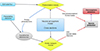 |
Figure 1 Schematic view of the Transolo simulation flow. Inputs are in blue and output in red. Taken from (Barthelemy et al., 2019). |
As shown in Figure 1, the energetic solar EUV fluxes and the precipitating electron fluxes are given as inputs to the code which then solves the transport equation for these electrons and returns as output the electron fluxes for given energy, pitch-angle and altitude grids. The code uses the DISORT routine (Stamnes et al., 1988) a discrete ordinate method, to solve the transport equation. The symmetry axis is the local magnetic field line. The code also requires atmospheric and ionospheric models to solve the transport equation. In our case, atmospheric model is NRLMSIS 2.0 (Emmert et al., 2021). It is also possible to use NRLMSIS 00 (Picone et al., 2002). The atmospheric model is parameterized by Ap and F10.7 indices and depends on the location on the Earth (latitude and longitude). The ionosphere composition and temperatures are computed using the IRI 2020 model (Bilitza et al., 2022).
As shown in Robert et al. (2023), for the 427.8 nm band, the shape of the electron energy distribution has a significant impact on the emission profiles and intensities. We may consider different analytical electron precipitation functions: mono-energetic, Maxwellian and Gaussian functions. The two first distributions are parameterized by the total precipitating energy (Etotal) and the mean energy of the distribution (Emoy). The Gaussian function needs a third parameter which is the width of the distribution. Since the Boltzman transport equation is linear, it is possible to study the effect of more complex distributions by summing the contributions of individual functions which may simulate different sources of precipitating electrons. This is important since the precipitating electron fluxes can often be the sum of several distributions with different mean energies as shown e.g. in Simon Wedlund et al. (2013) and Robert et al. (2023) revealing possible multiple sources and/or acceleration mechanisms.
Once the electron fluxes are calculated, a set of cross-sections is used to calculate the induced emissions. However the light emissions are not always directly resulting from an electron collision (primary or secondary electrons). Some chemistry processes need to be taken into account to get the full emission distribution. This is especially true for the O I red triplet (630–636–639 nm) and O I green line (557.7 nm) from atomic oxygen and the N I (520 nm) line for atomic nitrogen4. These transitions are forbidden in the electric dipole approximation as well as the N2 Vegard Kaplan vibronic transitions. Such transitions generally lead to metastable upper state of the considered transitions and thus long lifetime. Consequently, they are significantly quenched by collisions on neutral atoms, ions or molecules. This can strongly decrease the number of emitted photons when compared to the excitation of the upper level, especially at altitudes between 100 and 200 km. They are quoted with the word forbidden in the table summarizing all the considered transitions.
3.1 Input parameters and grids
This paper deals with the night-side auroral emissions meaning that we consider only electron precipitations as input and no solar EUV flux. The proton precipitations will be added in a further version of this work.
As mentioned above, the code uses the NRLMSIS 2.0 atmospheric model which is parametrized by F10.7 and Ap. In this paper, we use F10.7 = 158 and Ap = 80 which correspond to average conditions. It is important to notice that during intense precipitation events, the atmosphere is modified by the resultant chemistry and it can be convenient to artificially increase the Ap number to take into account these modifications as done in Robert et al. (2023). The code also needs the position on Earth (Latitude, Longitude) as an input for the NRLMSIS model and to calculate the magnetic field lines orientation. For the latter, we use IGRF-13 (Alken et al., 2021). An arbitrary magnetic field line orientation can also be considered. As a test case the following position was considered:
-
Latitude = 70° North,
-
Longitude = 20° East,
which corresponds to a location in the North of Scandinavia in the vicinity of the Tromso and Skibotn observatories in Northern Norway.
The simulation also requires the choice of the grids for the atmosphere, electrons energies and pitch-angles. We chose:
-
100 energies from 0.1 to 30000 eV. Logarithmic grid;
-
100 atmospheric layers from 80 to 520 km. Logarithmic grid;
-
32 pitch-angles, 16 down, 16 up distributed over all directions (0°–360°).
Due to the variation of the density of the atmosphere with the altitude, the grid step is not constant but logarithmic with smaller steps at low altitudes. It is similar for the energy grid since the main variations of the cross section due to electron impacts occurs between 20 eV and several hundreds of eV. The extrapolation at higher energy is done using power laws as proposed in the semi-classical theory of Bethe (Inokuti, 1971) and already considered in the previous versions of Transsolo. Even if we know that the precipitating particle fluxes can be the sum of several distributions with different total and mean energies (e.g. Simon Wedlund et al., 2013; Robert et al., 2023), we choose in this paper to study the effect of only a single distribution at once. And in order to accurately link the spectrum obtained with a specific energy of the precipitating electrons, we use mono-energetic electron beams at the top of the atmosphere. However for specific cases, Maxwellian or Gaussian distributions can also be used. In this last case, the width of the distribution has to be added as input parameter.
For the pitch-angle distribution at the top of the atmosphere, we use a Gaussian distribution of angles as described in Lilensten & Blelly (2002).
3.2 Electron impact cross sections and Franck-Condon factor for molecular bands
Each vibrational, vibronic or rovibronic5 transition cross section is related to the overlap of the vibrational wave function of each individual vibrational level. These overlaps are described by the Franck-Condon (FC) factors at first order6. The emission rates also depend on the excitation rate of the specific vibrational upper level of the transition which can be unknown. Therefore, we use the following strategy to calculate the transitions between two vibronic levels: if the cross sections versus energy are known, we use them. If not, the branching ratios can be calculated by using experimental laboratory spectra like those of Mangina et al. (2011). However, some weak transitions do not appear in these experimental spectra. For these ones, the cross section are obtained by using another transition with the same upper level and then use the FC factors ratio between the upper vibration level and the lower ones and compare them to the known one.
For a complete description, we need the full variation of the cross sections with the energy for the entire spectrum of the precipitating electrons. This variation is not complete for a large part of the emissions, especially for all the individual vibrational transitions. In this case, instead we use the hypothesis that the variation is similar to the full band excitation variation, i.e. that we consider a constant branching ratio with energy or if not available to the ionisation cross section variations. For example, if we compare the  first negative band cross section with the ionization one (Terrell et al., 2004), we can reasonably consider that their shapes are similar which allows validation of this hypothesis, at first order.
3.3 Line width
The line widths of the emissions are controlled by several parameters like the lifetime of the upper level and the thermal speed of the emitting species. We consider for each line a Gaussian shape with an adjustable width. For atomic species, the width is small and since we consider spectra acquired with medium resolution, we set arbitrarily the width of all the atomic lines to 0.2 nm (see Table 1).
For molecular transitions, since the vibronic transitions considered here contain unresolved rotational structures, the rotational temperatures strongly control the shape of the bands. These rotational temperatures have for example been studied by Jokiaho et al. (2008) for the first negative  band at 470.9 nm using high resolution (0.08 nm) measurements obtained with the High Throughput Imaging Echelle Spectrograph (HiTIES), from which they infer some energy characteristics of the precipitations in various types of aurora. To avoid complexity, we decide here to neglect these effects despite the very rich set of information they can carry. At this stage, considering that the high resolution is not our main target, we only separate the P and R branches for some molecular transitions of
  . However as shown in laboratory spectra (Mangina et al., 2011), the width of the P branch is much smaller than the one of the R branch. By fitting these laboratory spectra, we obtain a width of 0.567 nm for the R branch and 0.083 nm for the P branch for the entire
  first negative band. We similarly fitted the width for the other molecular bands and the resulting widths are given in Supplementary material. The Meinel band shows a very complex structure regarding the rotational levels with three branches heads. Less documented than the first negative band, we do not look at the detailed structure and we consider a wide Gaussian shape with a width of 3.3 nm which corresponds to a fit of the entire Meinel bands measured by Mangina et al. (2011). The width of the Vegard Kaplan band depends on the temperature as stated in Johnston et al. (1994) and shows an asymmetrical shape. In the code, we neglect the asymmetry and we use a Gaussian shape with 1.5 nm width which, according to Johnston et al. (1994) corresponds to a temperature ∼400 K which is close to typical thermospheric temperatures. The width can be modified in the code, for example 900 K temperature gives a 2 nm width.
It is important to keep in mind that the line width of each emission transition is a free parameter and can thus be adjusted very easily in the code, especially to fit low resolution instruments. In case of higher resolution instruments, it is important to keep in mind the hypothesis described above especially for the Meinel Band.
3.4 Comments on the red and green lines
Paradoxically the brightest and most famous auroral emission lines, the red and green lines from atomic oxygen, are among the most difficult to simulate since the number of processes that can create these lines is large. Several processes have some large uncertainties and make the calculation of these two lines very inaccurate. The simulations of these lines presented in this work are done to compare with results from other papers but must be taken cautiously.
For the green line, Whiter et al. (2023) show that we are currently not able to simulate and understand all the processes at its origin. Following their work, the calculated sources taken into account in our simulations of the green line (population of the O1 S level) are due to the following processes:
-
P1: electronic impact on O;
-
P2: electronic impact on O2;
-
P3: dissociative recombination of
 ;
; -
P4: collisional deactivation of
 ;
; -
P5: Collision of
 with N;
 -
P6: Barth mechanism (3 body process).
Besides the emission itself, the losses are the quenching by O and O2. The quenching of the O1 S state by N2 is negligible since the reaction rate is several orders of magnitude (3–5) lower than the quenching on O and O2 (Gronoff et al., 2008). The green line calculation takes into account the Barth mechanism despite the remaining questions regarding this process (Gronoff et al., 2008) and large uncertainties. All the references for reaction rates for the green line are identical to those in Whiter et al. (2023).
For the red line, the uncertainties are lower but as for the green line the chemical processes are important and thus the emissions are not directly linked to the electron precipitations. In addition, the excitation threshold for the red line is small (1.96 eV) such that it can be excited by the tail of the thermal electron population. In our simulations we consider the following creation processes:
-
P1: electronic impact on O;
-
P2: electronic impact on O2;
-
P3: dissociative recombination of
 ;
; -
P4: thermal electron impact;
-
P5: Collision of O2 with N+;
-
P6: Collision of O2 with N(2D).
The references for the red line creation processes are those listed in Solomon et al. (1988). The P2 process is negligible in the night side.
The loss processes are due to quenching with the different neutral species and the electrons. The reaction coefficients depend of the quenching species. They are given in Whiter et al. (2023) and Solomon et al. (1988) for the red and green lines respectively.
The problem is similar for the N I 520 nm with a much longer lifetime as mentioned in Section 2. We considered for this transition, the rates described in Rees & Romick (1985).
4 Results
4.1 Column integrated spectra
As an example, we show in Table 2 intensities of column integrated emissions for mono-energetic electrons with a mean energy of 0.1~keV, 1 keV and 10 keV and a total energy flux of 1 erg · cm−2 · s−1. This integration reproduces intensities that would be recorded by an instrument and is achieved by summing contributions from each individual volume emission rate calculated by the code along the intercepted field of view at each altitude of the grid. Column integrated intensities (C-Int-Int) give an indication on the variations of the emission with the mean energy of the precipitating electron distribution. For molecular bands, the code gives the intensity of each individual vibronic line. The spectra are given in Figures 2 and 3 for values of the mean energy equal to 1 keV and 10 keV. A vertical zoom-in (Intensity dimension) which allows better view of the large number of lines/bands is given in Figure 4 for a mean energy of 1 keV.
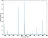 |
Figure 2 Spectrum for 1 keV and 1 erg · cm−2 · s−1 considering a mono-energetic input distribution. |
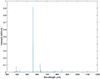 |
Figure 3 Spectrum for 10 keV and 1 erg · cm−2 · s−1 considering a mono-energetic input distribution. |
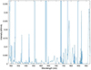 |
Figure 4 Spectrum for 1 keV and 1 erg · cm−2 · s−1 considering a mono-energetic input distribution. Zoom-in (Intensity dimension) of Figure 2. |
Column integrated intensity (C-Int-Int) of the main lines and bands in kR units. Values are presented for different mean energy of a mono-energetic electron distribution considering a fixed total energy flux of 1 erg · cm−2 · s−1 (which means a number of particles multiplied or divided by 10 for a mean energy of 10 and 0.1 keV respectively). For molecular lines, the values for the full band (FB) are given except for the 1st negative bands of  . The numbers in parentheses are the C-Int-Int obtained at constant number of particles compared to the case of 1 keV and 1 erg · cm−2 · s−1 (which corresponds to a total energy flux of 10 and 0.1 erg · cm−2 · s−1 respectively)
Table 2 provides a comparison of the emitted intensities for different mean energies considering either a constant total energetic flux or a constant total number of particles. For the first case, this could lead to counter-intuitive results since for example when the mean energy is multiplied by 10, this means that the number of particles is divided by 10. This is why e.g. at 10 keV, some intensities drop strongly due to both the variation of the cross-section and of the number of particles.
We notice that except for the green and red lines which are emitted by complex multi processes, the intensity variations are almost linear with the energy flux at a given mean energy.
If a Gaussian or Maxwellian distribution is considered, the variations of the intensities are significant but never exceed 20%.
4.2 Evolution of the spectrum as function of altitude
Since the code calculates the volume emission rates at different altitudes, it is possible to see how the emission spectrum evolves with the altitude which can be particularly useful for limb observations from space. The code also allows the determination of the altitude of the peak and the vertical thickness of the distribution. Robert et al. (2023) have shown the importance of these parameters for the reconstruction of particle precipitation characteristics. Figure 5 shows an example of the 3D simulated spectra where the intensity versus wavelength is also shown as function of the altitude. To look at more specific features (lines or bands) at various altitudes or to obtain a spectrum at a given altitude, cuts can be made in this 3D distribution. Figures 6 and 7 show for example the spectra at two different altitudes (114 and 221 km) while Figure 8 shows the altitude profiles of three different lines. We selected three lines directly related to electron precipitations, namely  427.8 nm line, the O I 844.6 nm line and the full first positive band of N2.
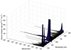 |
Figure 5 3D view of the synthetic spectra as function of the altitude for Emean = 7 keV and a total flux of 10 erg · cm−2 · s−1. The maximum volume emission rates shown are of 500 cm−3 · s−1 · nm−1 to allow a better visualization of the faint lines/bands. The computed maximum of the green line for this case is 2116 cm−3 · s−1 · nm−1. Note that the mean energy used here is larger than for the previous examples to allow a better discrimination of the altitude of each emission peak. |
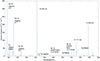 |
Figure 6 Spectrum at 114 km with the same parameters as in Figure 5. The green line peaks at 3432 cm−3 · s−1 · nm−1 and the |

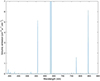 |
Figure 7 Spectrum at 221 km with the same parameters as in Figure 5. The intensity of the red line at 630 nm peaks at 65.3 cm−3 · s−1 · nm−1. |
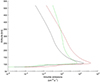 |
Figure 8 Altitude profiles of three emission lines directly linked with the electron precipitation: |

4.3 Uncertainties
There are a lot of parameters with poorly constrained uncertainties. For example, the uncertainties on the cross sections are at least of 10% (Terrell et al., 2004). The same paper even gives an uncertainty of 24% on the cross sections for the first negative band of  . Another major source of uncertainty is the atmospheric model. The NRLMSIS 2.0 model has uncertainties of the order of 10% (Emmert et al., 2021).
Considering the large number of uncertain parameters used in the simulations, an accurate estimate of the uncertainties on the emission intensities would require a complete study such as e.g. in the work of Gronoff et al. (2012) for the case of Mars. This is out of scope for this paper and will be the topic of a future paper. Instead we can try to give rough evaluations of the uncertainties on the different transitions.
As a first order estimate, it is reasonable to consider that the uncertainties of the simulations are between 20% and 30% for the intensity of each individual emission. The green line can even have higher uncertainties, especially at altitudes below 110 km for which modeling fails to reproduce the observations (Whiter et al., 2023). It is also important to note that the intensities of some lines/bands must have constant ratios like the 391.3, 427.8, 470 and 522 nm lines from  or the 630 and 636 nm red lines from atomic oxygen. These constant ratios are very useful to check the how the sensitivity of a given instrument varies with wavelength.
It is also important to mention that atmospheric models are generated using parameters like Ap or F10.7. However, when particle precipitations occur, the chemistry and composition of the upper atmosphere is modified. This effect is difficult to simulate but can have significant effects. Robert et al. (2023) artificially increased the Ap parameter in the atmospheric model to take into account this phenomenon but this cannot fully reproduce these complex interactions.
5 Implications for the green line polarisation
In a series of papers (Bosse et al., 2020, 2022a,b), it has been claimed that the green line at 557.7 nm is polarized at 2–5% and may be linked to ionospheric currents. According to the theoretical work by (Bommier et al., 2011), the green line cannot be polarized by impact with precipitating electrons since it is a transition between two singlet states (O1 S – O1 D). In order to solve this contradiction, (Bosse et al., 2022a) developed a sophisticated radiative transfer code to include (among others) scattering of light pollution by aerosols as a possible explanation of the observed polarization. Using single scattering, they showed that the contribution of light pollution scattering is not negligible but cannot reproduce completely the degrees and angles of polarisation they observed. There must be a polarisation source that is either intrinsic to the auroral emissions or occurs at auroral altitudes.
These polarisation measurements have been done using filters of 10 nm width (Full Width at Half Maximum). Hence, another plausible explanation could be that some lines with significant intensities appear in the band pass of the filter and would contribute partly or totally to the observed polarisation. In the spectral region around the green line (557.7 nm), we can identify the Δv = 1 bands of the first negative band of  , especially the (3–2), (2–1) and (1–0) bands at respectively 556, 559 and 563 nm which are the most powerful. For example, for a total energetic flux of 1 erg · cm−2 · s−1 and a mean energy of 200 eV, the simulations give 24 R for the full
  band while it gives 592 R for the green line. The 3 aforementioned bands represent roughly the third of the total band, so about 8 R or 1.3% of the green line intensity. Since the measured polarisation degree of the green line varies between 2% and 5%, it would require a very high polarisation rate of these bands to partly explain the measurements. Note that in the work of (Terrell et al., 2004), they made the assumption of an unpolarized band. Nevertheless, if these lines are polarised, it could explain partly the identified link with the currents mentioned by (Bosse et al., 2022b).
We can also note that the N2 first positive band branch with Δv = 5 contain emission bands between 550 and 563 nm. They have also been included in the calculations despite their weak cross sections. The calculated intensities are much fainter than the  bands. Some N I lines at 556 nm (Mangina et al., 2011) are also close to the green line but their intensities are also weak. It is important to notice that spectral measurements and simulations allow subtractions of the light pollution background easier than with photometers equipped with filters as shown in Barthelemy et al. (2011). The absolute calibration of the intensities are however much more complicated with spectrometers and they often present one unique field of view for one exposure. The solution of spectral imaging is then very promising but still heavy to implement.
6 Discussion and conclusions
Beyond the specific question of the polarisation of the green line, this work has the potential to better constrain which emissions can be present and mixed in measurements through a filter with a given bandwidth. The case of the Hα line at 656.2 nm is a good example since the mixing with other bands cannot be totally avoided even with very narrow filters. Therefore it is important to be able to simulate the other emissions knowing the characteristics of the precipitating particles using other emission lines. That way, a subtraction of the other contributions can in principle be made.
The tomographic reconstruction of the volume emission rates in one or two emission lines is a powerful tool to infer parameters of the precipitating particles as shown e.g. in Robert et al. (2023). But this technique cannot be applied everywhere. Taking auroral spectra is another way to bring additional constraints on the mean energy and fluxes of the precipitating particles on a single line-of-sight by comparing them with synthetic ones. Both techniques could also be used in parallel and comparisons of reconstructed parameters using the two techniques could be done along the line-of-sight of the spectrograph for cross-calibration and validation.
Another application of the synthetic spectra is to be able to simulate the full auroral spectrum in very different conditions in order to better design future instruments dedicated to auroral observations, especially spectrometers and spectro-imagers, like the WFAI-AOSI instrument (Wide Field Auroral Imager – Auroral Optical Spectral Imager), developed for the Aurora-D mission of the European Space Agency (Le Coarer et al., 2021).
In Cartwright (1978), the branching ratios within vibrational structure show small variations with the energy of the particles and therefore could be used in principle to add further constraints. This cannot be done with the simulations described here since we mainly consider constant branching ratios. Additional work could be to simulate the variations of the vibrational populations for different characteristic energy and to find proxies of the mean energy of the precipitating electrons distribution. The present paper can be considered as a basis for these future developments.
Finally, a last objective is to determine suitable candidates to compute line or band ratios and estimate the characteristic energy of the precipitating electrons from one or several of these ratios. For that purpose, simulations can be used and compared to either observations obtained with various filters whose spectral responses are known or with data from real spectrometers.
Acknowledgments
This work was supported by CNRS-INSU PNST (Programme National Soleil Terre) and the CNES Solar, Heliosphere, Magnetosphere (SHM) group. The authors thank Jean Lilensten for careful reading of the drafts of the paper and useful suggestions. The editor thanks two anonymous reviewers for their assistance in evaluating this paper.
Supplementary material
Supplementary Table: List of molecular bands taken into account with related branching ratios and line width. The branching ratios are determined by different method described in the text. For some transitions several values can be found in the literature. In this case, we kept the most recent ones. The widths are determined from experimental spectra when available. Lowest considered wavelength is 380 nm, highest is 900 nm. Access Supplementary Material
The ETRANS code mentioned in this paper is similar to the Transsolo code and is based on the same resolution principles. The cross sections can however be different.
For the reader not familiar with spectroscopic notations, we kindly refer them to any textbook in molecular spectroscopy, for example Tennyson (2019).
The code will be made available on request to the first author. Because of its complexity, a potential user of the code is requested to collaborate with the author to use it efficiently and avoid misuse.
All the references for cross sections are given in Table 1 and in Supplementary material.
In molecular spectroscopy, in the Born-Oppenheimer approximation, the electronic, vibrational and rotational degrees of freedom are decoupled. Vibronic means a transition mixing electronic and vibrational degrees of freedom and rovibronic mixes the three degrees of freedom mentioned above.
See for example Herzberg (1950) for additional information about Franck-Condon factors.
References
- Alken P, Thébault E, Beggan CD, Amit H, Aubert J, et al. 2021. International geomagnetic reference field: the thirteenth generation. Earth Planet Space 73(1): 49. https://doi.org/10.1186/s40623-020-01288-x. [CrossRef] [Google Scholar]
- Barthélemy M, Kalegaev V, Vialatte A, Le Coarer E, Kerstel E, et al. 2018. Amical sat and atise: two space missions for auroral monitoring. J Space Weather Space Clim 8: A44. https://doi.org/10.1051/swsc/2018035. [CrossRef] [EDP Sciences] [Google Scholar]
-
Barthelemy M, Lamy H, Vialatte A, Johnsen MG, Cessateur G, Zaourar N. 2019. Measurement of the polarisation in the auroral
 427.8 nm band. J Space Weather Space Clim 9: A26. https://doi.org/10.1051/swsc/2019024.
[CrossRef]
[EDP Sciences]
[Google Scholar]
427.8 nm band. J Space Weather Space Clim 9: A26. https://doi.org/10.1051/swsc/2019024.
[CrossRef]
[EDP Sciences]
[Google Scholar]
- Barthelemy M, Lilensten J, Pitout F, Simon Wedlund C, Thissen R, et al. 2011. Polarisation in the auroral red line during coordinated EISCAT Svalbard Radar/optical experiments. Ann Geophys 29(6): 1101–1112. https://doi.org/10.5194/angeo-29-1101-2011. [CrossRef] [Google Scholar]
- Bilitza D, Pezzopane M, Truhlik V, Altadill D, Reinisch BW, Pignalberi A. 2022. The international reference ionosphere model: a review and description of an ionospheric benchmark. Rev Geophys 60(4): e2022RG000792. https://doi.org/10.1029/2022RG000792. [CrossRef] [Google Scholar]
- Bommier V, Sahal-Bréchot S, Dubau J, Cornille M. 2011. The theoretical impact polarization of the O I 6300 Å red line of Earth aurorae. Ann Geophys 29(1): 71–79. https://doi.org/10.5194/angeo-29-71-2011. [CrossRef] [Google Scholar]
- Bosse L, Lilensten J, Gillet N, Brogniez C, Pujol O, Rochat S, Delboulbé A, Curaba S, Johnsen MG. 2022a. At the source of the polarisation of auroral emissions: experiments and modeling. J Space Weather Space Clim 12: 7. https://doi.org/10.1051/swsc/2022004. [CrossRef] [EDP Sciences] [Google Scholar]
- Bosse L, Lilensten J, Gillet N, Rochat S, Delboulbé A, et al. 2020. On the nightglow polarisation for space weather exploration. J Space Weather Space Clim, 10: 35. https://doi.org/10.1051/swsc/2020036. [CrossRef] [EDP Sciences] [Google Scholar]
- Bosse L, Lilensten J, Johnsen MG, Gillet N, Rochat S, Delboulbé A, Curaba S, Ogawa Y, Derverchère P, Vauclair S. 2022b. The polarisation of auroral emissions: a tracer of the E region ionospheric currents. J Space Weather Space Clim 12: 17. https://doi.org/10.1051/swsc/2022014. [CrossRef] [EDP Sciences] [Google Scholar]
- Broadfoot AL, Hatfield DB, Anderson ER, Stone TC, Sandel BR, Gardner JA, Murad E, Knecht DJ, Pike CP, Viereck RA. 1997. N2 triplet band systems and atomic oxygen in the dayglow. J Geophys Res 102(A6): 11567–11584. https://doi.org/10.1029/97JA00771. [CrossRef] [Google Scholar]
- Cartwright DC. 1978. Vibrational populations of the excited states of N2 under auroral conditions. J Geophys Res 83(A2): 517–531. https://doi.org/10.1029/JA083iA02p00517. [CrossRef] [Google Scholar]
- Cartwright DC, Brunger MJ, Campbell L, Mojarrabi B, Teubner PJO. 2000. Nitric oxide excited under auroral conditions: Excited state densities and band emissions. J Geophys Res Space Phys 105(A9): 20857–20867. https://doi.org/10.1029/1999JA000333. [CrossRef] [Google Scholar]
- Degen V. 1982. Synthetic spectra for auroral studies: the N2 Vegard-Kaplan band system. J Geophys Res 87(12): 10541–10547. https://doi.org/10.1029/JA087iA12p10541. [CrossRef] [Google Scholar]
- Emmert JT, Drob DP, Picone JM, Siskind DE, Jones M, et al. 2021. NRLMSIS 2.0: a whole atmosphere empirical model of temperature and neutral species densities. Earth Space Sci 8(3): e01321. https://doi.org/10.1029/2020EA001321. [CrossRef] [Google Scholar]
- Frey HU, Mende SB, Meier RR, Kamaci U, Urco JM, Kamalabadi F, England SL, Immel TJ. 2023. In flight performance of the far ultraviolet instrument (FUV) on ICON. Space Sci Rev 219(3): 23. https://doi.org/10.1007/s11214-023-00969-9. [CrossRef] [Google Scholar]
- Gattinger RL, Vallance Jones A. 1974. Quantitative spectroscopy of the aurora. II – The spectrum of medium intensity aurora between 4500 and 8900 A. Can J Phys 52: 2343–2356. https://doi.org/10.1139/p74-305. [CrossRef] [Google Scholar]
- Gattinger RL, Vallance Jones A, Degenstein DA, Llewellyn EJ. 2010. Quantitative spectroscopy of the aurora. VI. The auroral spectrum from 275 to 815 nm observed by the OSIRIS spectrograph on board the Odin spacecraft. Can J Phys 88(8): 559–567. https://doi.org/10.1139/P10-037. [CrossRef] [Google Scholar]
- Gillies DM, Donovan E, Hampton D, Liang J, Connors M, Nishimura Y, Gallardo-Lacourt B, Spanswick E. 2019. First observations from the TREx spectrograph: the optical spectrum of STEVE and the Picket fence phenomena. Geophys Res Lett 46(13): 7207–7213. https://doi.org/10.1029/2019GL083272. [CrossRef] [Google Scholar]
- Gilmore FR, Laher RR, Espy PJ. 1992. Franck–Condon factors, r-centroids, electronic transition moments, and Einstein coefficients for many nitrogen and oxygen band systems. J Phys Chem Ref Data 21(5): 1005–1107. https://doi.org/10.1063/1.555910. [CrossRef] [Google Scholar]
- Gronoff G, Lilensten J, Simon C, Barthélemy M, Leblanc F, Dutuit O. 2008. Modelling the Venusian airglow. A&A 482(3): 1015–1029. https://doi.org/10.1051/0004-6361:20077503. [CrossRef] [EDP Sciences] [Google Scholar]
- Gronoff G, Simon Wedlund C, Mertens CJ, Barthélemy M, Lillis RJ, Witasse O. 2012. Computing uncertainties in ionosphere-airglow models: II. The Martian airglow. J Geophys Res Space Phy 117(A5): A05309. https://doi.org/10.1029/2011JA017308. [Google Scholar]
- Grubbs G, Michell R, Samara M, Hampton D, Hecht J, Solomon S, Jahn J-M. 2018. A comparative study of spectral auroral intensity predictions from multiple electron transport models. J Geophys Res Space Phys 123(1): 993–1005. https://doi.org/10.1002/2017JA025026. [CrossRef] [Google Scholar]
- Herlingshaw K, Partamies N, van Hazendonk C, Syrjäsuo M, Baddeley L, et al. 2024. Science highlights from the Kjell Henriksen Observatory on Svalbard. Arctic Sci 11, 1–25. https://doi.org/10.1139/as-2024-0009. [Google Scholar]
- Herzberg G. 1950. Molecular spectra and molecular structure. Vol. 1: Spectra of diatomic molecules, Van Nostrand, New York. [Google Scholar]
- Inokuti M. 1971. Inelastic collisions of fast charged particles with atoms and molecules – the Bethe theory revisited. Rev Mod Phys 43: 297–347. https://doi.org/10.1103/RevModPhys.43.297. [CrossRef] [Google Scholar]
- Itikawa Y. 2006. Cross sections for electron collisions with nitrogen molecules. J Phys Chem Ref Data 35(1): 31–53. https://doi.org/10.1063/1.1937426. [CrossRef] [Google Scholar]
- Itikawa Y, Ichimura A, Onda K, Sakimoto K, Takayanagi K, Hatano Y, Hayashi M, Nishimura H, Tsurubuchi S. 1989. Cross sections for collisions of electrons and photons with oxygen molecules. J Phys Chem Ref Data 18(1): 23–42. https://doi.org/10.1063/1.555841. [CrossRef] [Google Scholar]
- Johnston JE, Hatfield DB, Lyle Broadfoot A. 1994. Synthetic spectra for the Arizona airglow experiment. In: Optical spectroscopic techniques and instrumentation for atmospheric and space research, vol. 2266, Wang J, Hays PB (Ed.), International Society for Optics and Photonics, SPIE, pp. 480–491. https://doi.org/https://doi.org/10.1117/12.187559. [CrossRef] [Google Scholar]
-
Jokiaho O, Lanchester BS, Ivchenko N. 2009. Resonance scattering by auroral
 : steady state theory and observations from svalbard. Ann Geophys 27(9): 3465–3478. https://doi.org/10.5194/angeo-27-3465-2009.
[CrossRef]
[Google Scholar]
: steady state theory and observations from svalbard. Ann Geophys 27(9): 3465–3478. https://doi.org/10.5194/angeo-27-3465-2009.
[CrossRef]
[Google Scholar]
-
Jokiaho O, Lanchester BS, Ivchenko N, Daniell GJ, Miller LCH, Lummerzheim D. 2008. Rotational temperature of
 (0,2) ions from spectrographic measurements used to infer the energy of precipitation in different auroral forms and compared with radar measurements. Ann Geophys 26(4): 853–866. https://doi.org/10.5194/angeo-26-853-2008.
[CrossRef]
[Google Scholar]
(0,2) ions from spectrographic measurements used to infer the energy of precipitation in different auroral forms and compared with radar measurements. Ann Geophys 26(4): 853–866. https://doi.org/10.5194/angeo-26-853-2008.
[CrossRef]
[Google Scholar]
- Khazanov GV, Koen MA, Burenkov SI. 1979. Numerical solution of the kinetic equation for photoelectrons in the plasmosphere with account for free and captured zones. Kosmicheskie Issledovaniia 17: 894–900. [Google Scholar]
- Kirillov AS, Belakhovsky VB, Maurchev EA, Balabin YuV, Germanenko AV, Gvozdevskiy BB. 2021. Luminescence of molecular nitrogen and molecular oxygen in the earth’s middle atmosphere during the precipitation of high-energy protons, Geomagn Aeron 61(6): 864–870. https://doi.org/10.1134/S0016793221060086. [CrossRef] [Google Scholar]
- Kramida A, Ralchenko Yu, Reader J, NIST ASD Team. 2022. NIST Atomic Spectra Database (ver. 5.10) [Online], National Institute of Standards and Technology, Gaithersburg, MD. Available at https://physics.nist.gov/asd (accessed October 30, 2023). [Google Scholar]
- Lanchester B, Gustavsson B. 2012. Imaging of aurora to estimate the energy and flux of electron precipitation. Geophys Monog Ser 197: 171–182. https://doi.org/10.1029/2011GM001161. [Google Scholar]
- Le Coarer EP, Richard L, Robert E, Rodrigo J, Sequies T, et al. 2021. Optimization of a compact static interferometer based on ImSPOC technology for a wide field polar lights monitoring. In: International Conference on Space Optics – ICSO 2020, , vol. 11852, Cugny B, Sodnik Z, Karafolas N (Ed.), International Society for Optics and Photonics, SPIE, p. 118521G. https://doi.org/10.1117/12.2599241. [Google Scholar]
- Lilensten J, Blelly PL. 2002. The TEC and F2 parameters as tracers of the ionosphere and thermosphere. J Atmos Sol Terr Phys 64(7): 775–793. https://doi.org/10.1016/S1364-6826(02)00079-2. [CrossRef] [Google Scholar]
- Lilensten J, Moen J, Barthélemy M, Thissen R, Simon C, Lorentzen DA, Dutuit O, Amblard PO, Sigernes F. 2008. Polarization in aurorae: a new dimension for space environments studies. Geophys Res Lett 35(8): L08804. https://doi.org/10.1029/2007GL033006. [CrossRef] [Google Scholar]
- Lofthus A, Krupenie PH. 1977. The spectrum of molecular nitrogen. J Phys Chem Ref Data 6(1): 113–307. https://doi.org/10.1063/1.555546. [CrossRef] [Google Scholar]
- Lummerzheim D, Lilensten J. 1994. Electron transport and energy degradation in the ionosphere: Evaluation of the numerical solution, comparison with laboratory experiments and auroral observations. Ann Geophys 12(10–11): 1039–1051. https://doi.org/10.1007/s00585-994-1039-7. [CrossRef] [Google Scholar]
- Lummerzheim D, Rees MH, Romick GJ. 1990. The application of spectroscopic studies of the aurora to thermospheric neutral composition. Planet Space Sci 38(1): 67–78. https://doi.org/10.1016/0032-0633(90)90006-C. [CrossRef] [Google Scholar]
- Mangina RS, Ajello JM, West RA, Dziczek D. 2011. High-resolution electron-impact emission spectra and vibrational emission cross sections from 330–1100 nm for N2 . Astrophys J Suppl 196(1): 13. https://doi.org/10.1088/0067-0049/196/1/13. [CrossRef] [Google Scholar]
- Marchaudon A, Blelly PL. 2020. Impact of the dipole tilt angle on the ionospheric plasma as modeled with IPIM. J Geophys Res Space Phys 125(6): e27672. https://doi.org/10.1029/2019JA027672. [CrossRef] [Google Scholar]
- Oyama SI, Tsuda TT, Hosokawa K, Ogawa Y, Miyoshi Y, et al. 2018. Auroral molecular-emission effects on the atomic oxygen line at 777.4 nm. Earth Planet Space 70(1): 166. https://doi.org/10.1186/s40623-018-0936-z. [CrossRef] [Google Scholar]
- Picone JM, Hedin AE, Drob DP, Aikin AC. 2002. NRLMSISE-00 empirical model of the atmosphere: Statistical comparisons and scientific issues. J Geophys Res Space Phys 107(12): 1468. https://doi.org/10.1029/2002JA009430. [Google Scholar]
-
Piper LG, Green BD, Blumberg WAM, Wolnik SJ. 1986. Electron impact excitation of the
 meinel band. J. Phys. B: At. Mol. Opt. Phys 19(20): 3327. https://doi.org/10.1088/0022-3700/19/20/015.
[CrossRef]
[Google Scholar]
meinel band. J. Phys. B: At. Mol. Opt. Phys 19(20): 3327. https://doi.org/10.1088/0022-3700/19/20/015.
[CrossRef]
[Google Scholar]
- Rees MH, Romick GJ. 1985. Atomic nitrogen in aurora: production, chemistry, and optical emissions. J Geophys Res 90(10): 9871–9880. https://doi.org/10.1029/JA090iA10p09871. [CrossRef] [Google Scholar]
- Robert E, Barthelemy M, Cessateur G, Woelfflé A, Lamy H, Bouriat S, Johnsen MG, Brändström U, Biree L. 2023. Reconstruction of electron precipitation spectra at the top of the upper atmosphere using 427.8 nm auroral images. J Space Weather Space Clim 13: 30. https://doi.org/10.1051/swsc/2023028. [CrossRef] [EDP Sciences] [Google Scholar]
- Simon Wedlund C, Lamy H, Gustavsson B, Sergienko T, Brändström U. 2013. Estimating energy spectra of electron precipitation above auroral arcs from ground-based observations with radar and optics. J Geophys Res Space Phys 118(6): 3672–3691. https://doi.org/10.1002/jgra.50347. [CrossRef] [Google Scholar]
-
Slanger TG, Cosby PC, Huestis DL. 2003. A new O2 band system: The
 transition in the terrestrial nightglow. J Geophys Res Space Phys 108(A2): 1089. https://doi.org/10.1029/2002JA009677.
[Google Scholar]
transition in the terrestrial nightglow. J Geophys Res Space Phys 108(A2): 1089. https://doi.org/10.1029/2002JA009677.
[Google Scholar]
- Solomon SC. 2001. Auroral particle transport using Monte Carlo and hybrid methods. J Geophys Res 106(A1): 107–116. https://doi.org/10.1029/2000JA002011. [CrossRef] [Google Scholar]
- Solomon SC. 2017. Global modeling of thermospheric airglow in the far ultraviolet. J Geophys Res Space Phys 122(7): 7834–7848. https://doi.org/10.1002/2017JA024314. [CrossRef] [Google Scholar]
- Solomon SC, Hays PB, Abreu VJ. 1988. The auroral 6300 Å emission: observations and modeling. J Geophys Res Space Phys 93(9): 9867–9882. https://doi.org/10.1029/JA093iA09p09867. [CrossRef] [Google Scholar]
- Stamnes K, Tsay S-C, Wiscombe W, Jayaweera K. 1988.Numerically stable algorithm for discrete-ordinate-method radiative transfer in multiple scattering and emitting layered media. Appl Opt 27(12): 2502–2509. [CrossRef] [Google Scholar]
- Tennyson J. 2019. Astronomical spectroscopy: an introduction to the atomic and molecular physics of astronomical spectroscopy. 3rd edn, World Scientific, https://doi.org/10.1142/7574. [CrossRef] [Google Scholar]
- Terrell CA, Hansen DL, Ajello JM. 2004. The near-ultraviolet and visible emission spectrum of O2 by electron impact. J Phys B At Mol Opt Phys 37(9): 1931. https://doi.org/10.1088/0953-4075/37/9/013. [CrossRef] [Google Scholar]
- Tuttle S, Lanchester B, Gustavsson B, Whiter D, Ivchenko N, Fear R, Lester M. 2020. Horizontal electric fields from flow of auroral O+(2P) ions at sub-second temporal resolution. Ann Geophys 38(4): 845–859. https://doi.org/10.5194/angeo-38-845-2020. [CrossRef] [Google Scholar]
- Vallance Jones A, Gattinger RL. 1972. Quantitative spectroscopy of the aurora. I. The spectrum of bright aurora between 7000 and 9000 Å at 7.5 Å resolution. Can J Phys 50: 1833–1841. https://doi.org/10.1139/p72-249. [CrossRef] [Google Scholar]
- Vialatte A. 2017. Effets des entrées énergétiques sur les composés azotés dans la haute atmosphère de la Terre. PhD thesis. Thèse de doctorat dirigée par Barthelemy, Mathieu Astrophysique et milieux dilues Université Grenoble Alpes (ComUE). Available at http://www.theses.fr/2017GREAY066. [Google Scholar]
- Vialatte A, Barthélemy M, Lilensten J. 2017. Impact of energetic electron precipitation on the upper atmosphere: nitric monoxide. Open Atmos Sci J 11(1): 88–104. https://doi.org/10.2174/1874282301711010088. [CrossRef] [Google Scholar]
-
Whiter DK, Partamies N, Gustavsson B, Kauristie K. 2023. The altitude of green OI 557.7 nm and blue
 427.8 nm aurora. Ann Geophys 41(1): 1–12. https://doi.org/10.5194/angeo-41-1-2023.
[CrossRef]
[Google Scholar]
427.8 nm aurora. Ann Geophys 41(1): 1–12. https://doi.org/10.5194/angeo-41-1-2023.
[CrossRef]
[Google Scholar]
Cite this article as: Mathieu B, Robert E & Lamy H. 2025. Synthetic spectra of the aurora: N2, N2+, N, N+, O2+ and O emissions. J. Space Weather Space Clim. 15, 19. https://doi.org/10.1051/swsc/2025013.
All Tables
Column integrated intensity (C-Int-Int) of the main lines and bands in kR units. Values are presented for different mean energy of a mono-energetic electron distribution considering a fixed total energy flux of 1 erg · cm−2 · s−1 (which means a number of particles multiplied or divided by 10 for a mean energy of 10 and 0.1 keV respectively). For molecular lines, the values for the full band (FB) are given except for the 1st negative bands of . The numbers in parentheses are the C-Int-Int obtained at constant number of particles compared to the case of 1 keV and 1 erg · cm−2 · s−1 (which corresponds to a total energy flux of 10 and 0.1 erg · cm−2 · s−1 respectively)
All Figures
|
Figure 1 Schematic view of the Transolo simulation flow. Inputs are in blue and output in red. Taken from (Barthelemy et al., 2019). |
| In the text | |
|
Figure 2 Spectrum for 1 keV and 1 erg · cm−2 · s−1 considering a mono-energetic input distribution. |
| In the text | |
|
Figure 3 Spectrum for 10 keV and 1 erg · cm−2 · s−1 considering a mono-energetic input distribution. |
| In the text | |
|
Figure 4 Spectrum for 1 keV and 1 erg · cm−2 · s−1 considering a mono-energetic input distribution. Zoom-in (Intensity dimension) of Figure 2. |
| In the text | |
|
Figure 5 3D view of the synthetic spectra as function of the altitude for Emean = 7 keV and a total flux of 10 erg · cm−2 · s−1. The maximum volume emission rates shown are of 500 cm−3 · s−1 · nm−1 to allow a better visualization of the faint lines/bands. The computed maximum of the green line for this case is 2116 cm−3 · s−1 · nm−1. Note that the mean energy used here is larger than for the previous examples to allow a better discrimination of the altitude of each emission peak. |
| In the text | |
|
Figure 6 Spectrum at 114 km with the same parameters as in Figure 5. The green line peaks at 3432 cm−3 · s−1 · nm−1 and the |
| In the text | |
|
Figure 7 Spectrum at 221 km with the same parameters as in Figure 5. The intensity of the red line at 630 nm peaks at 65.3 cm−3 · s−1 · nm−1. |
| In the text | |
|
Figure 8 Altitude profiles of three emission lines directly linked with the electron precipitation: |
| In the text | |
Current usage metrics show cumulative count of Article Views (full-text article views including HTML views, PDF and ePub downloads, according to the available data) and Abstracts Views on Vision4Press platform.
Data correspond to usage on the plateform after 2015. The current usage metrics is available 48-96 hours after online publication and is updated daily on week days.
Initial download of the metrics may take a while.