| Issue |
J. Space Weather Space Clim.
Volume 15, 2025
|
|
|---|---|---|
| Article Number | 23 | |
| Number of page(s) | 17 | |
| DOI | https://doi.org/10.1051/swsc/2025019 | |
| Published online | 04 June 2025 | |
Research Article
Assimilation of the total electron content obtained from GNSS to a model of the ionosphere using a hierarchical Bayesian network
1
Faculty of Land Resources Engineering, Kunming University of Science and Technology, Kunming 650093, PR China
2
Changsha Uranium Geology Research Institute, CNNC, Changsha, 410007, PR China
* Corresponding author: This email address is being protected from spambots. You need JavaScript enabled to view it.
Received:
29
May
2024
Accepted:
2
May
2025
Abstract
Ionospheric data assimilation aims to address the uneven spatiotemporal distribution of observational data and errors in numerical models. This paper proposes an ionospheric data assimilation model using the hierarchical Bayesian network (HBN) algorithm. We use the International Reference Ionosphere (IRI) 2016 as a background model. The HBN method assimilates global navigation satellite system (GNSS) observational data from approximately 260 stations within the Crustal Movement Observation Network of China (CMONOC). For this analysis, we use the total electron content (TEC) data from the Center for Orbit Determination in Europe (CODE) and BeiDou Navigation Satellite System (BDS) geostationary earth orbit (GEO) experiments. We evaluate the HBN assimilation effect through single-frequency precise point positioning (PPP). The results demonstrate that the HBN algorithm closely aligns with the BDS GEO TEC, regardless of geomagnetic conditions. Statistical results show that, with BDS GEO TEC data as the ground truth reference, the HBN model improves the correlation coefficient by approximately 14% and reduces the root mean square error (RMSE) by around 33% compared to the IRI model. The assimilation effect is significantly superior to that of the Kalman filter. Additionally, the HBN-based PPP method demonstrates slightly improved GNSS positioning accuracy compared to CODE-based PPP, with a reduction in RMSE observed under both geomagnetically disturbed and quiet conditions. Thus, the HBN method is effective for ionospheric data assimilation.
Key words: Ionosphere / Data assimilation / Hierarchical Bayesian network algorithm / Global navigation satellite system / Total electron content
© J. Tang et al., Published by EDP Sciences 2025
 This is an Open Access article distributed under the terms of the Creative Commons Attribution License (https://creativecommons.org/licenses/by/4.0), which permits unrestricted use, distribution, and reproduction in any medium, provided the original work is properly cited.
1 Introduction
High-precision ionospheric models are critical in the global navigation satellite system (GNSS), significantly improving positioning accuracy, mitigating multi-path effects, and correcting satellite clock ersrors (Yuan et al., 2019; Gu et al., 2021). Total electron content (TEC) refers to the total number of electrons in a one-square-meter cross-section column along the path between a satellite and the GNSS receiver. It is one of the crucial parameters for describing the ionosphere’s influence on GNSS signals. Solar activity affects radio communications, satellite navigation, and even geomagnetically induced currents. Accurate ionospheric TEC models are therefore essential for effective monitoring and correction during solar disturbances. Researchers have developed several real-time monitoring, inversion, and regional or global TEC models to describe the TEC distribution accurately (Mao et al., 2008; Mukhtaro et al., 2013). However, both empirical and physical ionospheric models still have certain limitations when dealing with the real-time TEC field in the ionosphere. To improve the practicality of these TEC models and fully use observational data, despite their uneven spatial and temporal distribution, data assimilation techniques have been introduced from meteorology into the field of real-time ionospheric TEC. Data assimilation enables the integration of observational data into model predictions, enhancing model accuracy and adaptability under varying ionospheric conditions. Through data assimilation, it is possible to interpolate, extrapolate, and aggregate observational data, effectively merging redundant or conflicting observations into the best estimate (Hajj et al., 2004; Forootan et al., 2021; Kosary et al., 2022). Consequently, assimilation techniques enable an accurate description of the distribution and variation of TEC in the ionosphere. Using assimilation techniques and integrating multiple data sources enables the establishment of a real-time TEC model. This model can accurately reflect observational data and meet the requirements of ionospheric space weather monitoring. Data assimilation, while a powerful tool, is not without its limitations. Assimilation models typically rely on high-quality observational data, and high-resolution assimilation models demand substantial computational resources, which may introduce delays in real-time monitoring. Additionally, data assimilation methods may struggle in regions with sparse observational data, where the lack of input can lead to inaccuracies in model predictions. Model assumptions and simplifications, such as linearization and approximations, can also introduce biases, especially in highly dynamic or irregular ionospheric conditions. These limitations highlight the need for ongoing improvements in data acquisition and assimilation algorithms to enhance accuracy and computational efficiency (Grynyshyna-Poliuga, 2024).
In recent years, numerous global and regional ionospheric TEC assimilation methods have been developed to forecast ionospheric space weather (Fuller-Rowell et al., 2006; Gardner et al., 2014; Ssessanga et al., 2019; Chen et al., 2020). Methods such as the variational algorithm, Kalman filter (KF), and ensemble KF have proven highly effective and accurate. Schunk et al. (2004) developed a data assimilation model, Global Assimilation of Ionospheric Measurements, based on a physics-based ionospheric model and KF. This model is used to simulate both the ionosphere and the neutral atmosphere. Aa et al. (2015), using a KF data assimilation approach, assimilated GNSS data and established a TEC map for the Chinese region with a spatial resolution of 1° × 1° and a temporal resolution of 5 min. They demonstrated the effectiveness of this method in providing an accurate regional distribution of ionospheric TEC. Lin et al. (2017) employed a Gaussian-Markov KF method to assimilate TEC data observed by ground-based global positioning system receivers and space-based radio occultation instruments into the International Reference Ionosphere (IRI). Subsequently, Qiao et al. (2021) developed a TEC model for China and neighboring regions using the Gaussian-Markov KF approach.
Wikle & Berliner (2007) proposed using hierarchical spatiotemporal models to enable more flexible analysis of environmental data distributed across space and time. To model delicate particulate matter, McMillan et al. (2010) employed a hierarchical Bayesian framework utilizing Markov chain Monte Carlo (MCMC) techniques to model the underlying uncertainty in environmental data. Their approach successfully demonstrated the ability to improve predictive accuracy and quantify model uncertainty. However, the method was limited by its high computational complexity and dependence on prior assumptions, which may restrict its scalability in large datasets or applications with limited prior information. Rayner (2020) used a hierarchical modeling approach to establish an atmospheric tracking model. It treats both parameters and models as random variables. Song & Mallick (2019) applied multi-level Bayesian model regularization to spatially observed and predicted unobserved curves. Compared to the Kalman algorithm, which only estimates mean and variance, the hierarchical Bayesian network (HBN) can sample through Monte Carlo to obtain posterior probability distributions of states and parameters. This capability allows it to better describe the temporal changes in non-linear systems over time (Qin et al., 2009). Traditional data assimilation processes, represented by KF, often involve specific parameters determined by prior knowledge or defined as constants throughout the assimilation process, such as the error variance of observational data and model prediction values. These assumptions significantly limit the algorithm’s consideration of uncertainty.
In contrast, hierarchical modeling theory in data assimilation decomposes the problem hierarchically, leveraging conditional probability to represent the spatial dependencies of state variables. This approach overcomes the restriction of spatial independence requirements. Unlike the KF family of algorithms, the HBN algorithm overcomes the limitations of linear variation in the system state and the assumption that errors follow a Gaussian distribution (Tang et al., 2022). Additionally, parameters representing spatial dependencies can vary over time in Bayesian networks, exhibiting significant potential for application in spatiotemporal analysis. HBN can handle data from different sources and resolutions without requiring forced changes in data resolution through resampling. In the context of HBN, solving complex posterior probability problems is transformed into a series of more straightforward posterior probability solutions, easily achievable through Monte Carlo sampling methods. The IRI-2016 model was selected as the background model due to its widely recognized reliability and accuracy in representing the climatological features of global and regional ionospheric characteristics. It is well-suited for data assimilation techniques, enhancing TEC prediction accuracy. Moreover, the IRI model has been extensively validated in GNSS research and can adapt to the time-varying characteristics of the ionosphere, making it a robust foundation for this study (An et al., 2020; Peng et al., 2024).
In this study, the Center for Orbit Determination in Europe (CODE) is used as one of the ground truth references. The CODE TEC is a global ionospheric TEC model developed by the CODE at the University of Bern, Switzerland. It is derived from actual GNSS observations collected from global ground-based stations. The model generates global TEC distributions using spherical harmonic analysis and interpolation techniques. While land regions benefit from dense observational data, TEC values over oceanic regions are primarily estimated through interpolation. CODE TEC offers high spatial and temporal resolution and is widely applied in ionospheric research, satellite navigation accuracy enhancement, and space weather monitoring (Xiong et al., 2022).
This study presents an ionospheric TEC model based on the HBN theory. The TEC observations from the Crustal Movement Observation Network of China (CMONOC) are assimilated into the IRI-2016 model. The assimilation results are evaluated using TEC estimates from the BeiDou Navigation Satellite System (BDS) geostationary orbit (GEO) and TEC products from CODE. A comparative analysis of the differences between the HBN and KF models is conducted. Finally, this research employs single-frequency precise point positioning (PPP) to validate the reliability of HBN in practical GNSS applications.
2 Methodology
In the framework of the HBN theory, data assimilation is decomposed into three layers: data, process, and parameters. The data layer includes site observational data and empirical model data. The process layer represents the spatiotemporal distribution and variations of the parameters to be assimilated. The parameters layer includes all parameters involved in the previous two layers. The HBN algorithm treats data, process, and parameters as three random variables, establishing conditional probability models for each. Establishing a conditional probability model transforms the problem of data assimilation into an inference process whereby the posterior probability distribution of parameters under given conditions is obtained.
Once the definitions of the data model, process model, and parameter model are established, it is possible to infer the posterior distributions of the process and parameters:
 (1)
(1)
Simultaneously, the data, process, and parameter models can be hierarchically decomposed into simpler models according to the hierarchical modeling theory (Banerjee et al., 2003). It is therefore possible to define complex models in hierarchical modeling theory by establishing multiple levels of simpler models.
The algorithmic flow of the HBN is depicted in Figure 1, illustrating the sequence of operations, including data preparation, network learning and validation, and prediction. Once the validation accuracy meets the requisite standards, the network can be employed for TEC assimilation at any point.
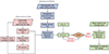 |
Figure 1 HBN ionospheric data assimilation process. Red represents the observation preparation, blue denotes the background data preparation, and green indicates the HBN computation. |
2.1 Data model
The data model p(data|process, parameters) describes the generation of observed data by establishing relationships between the observed data and the underlying real processes and associated parameters. This approach allows for the quantification and modeling of the inherent uncertainty present in the observed data. HBN assumes that, at any given moment, a true value exists that is not directly observable. The ultimate objective of data assimilation is to combine observational data with model predictions to infer the posterior probability distribution of the target variable, or the “true value”. The posterior distribution provides the “most probable value” and quantifies the uncertainty range, representing the error margin. Assume that data Xi represents datasets at different spatial resolutions Yi. Here, Yi serves as a critical variable to capture and model the spatial characteristics of datasets at different resolutions, forming the basis for subsequent integration into the process model. θD represents the parameters of the data model, characterizing the spatial and temporal features of the observational data. Given X = (X1, X2, …, Xn), Y = (Y1, Y2, …, Yn), and  , the data model is thus defined as follows:
 (2)
(2)
In the equation, HBN constructs a distinct model  for each dataset with a different resolution, ensuring that datasets with varying resolutions are appropriately represented within the process model. This demonstrates the advantage of HBN in handling data with resolution discrepancies.
2.2 Process model
Process models describe the processes of assimilation to spatial and temporal variables. The definition of the process model largely depends on using prior knowledge and data analysis. The purpose of establishing a process model is to describe the spatiotemporal distribution and variations of ionospheric TEC. The process model  , similar to the data model, can be decomposed into several sub-models based on conditional independence. The process model is defined as:
 (3)
(3)
When data sources from different platforms and with varying resolutions are available, the task of the process model is to integrate these data into a unified framework. This ensures that data from each source or resolution can be consistently represented within the same process model.
2.3 Parameter model
The parameter model defines the prior distribution probabilities for all parameters in the data model and the process model. Like the data model and process model, the parameter model can be decomposed into several models. In practical applications, it is often assumed that the parameter models are mutually independent.  is a vector comprising multiple sub-parameters, which are used to characterize features across different data sources. θp represents the parameters of the process model.
  is a vector in which each sub-parameter represents the true state or physical process underlying the data. Based on the independence assumption, the joint prior distribution can be decomposed into the independent distributions of each parameter as follows:
 (4)
(4)
Data analysis or other research results usually determine the distribution of prior probabilities for parameters (Carlin & Banerjee, 2003). This study uses conjugate priors to express the prior probability distributions of parameters, facilitating computational efficiency. Specifically, when a conjugate prior is used, the posterior distribution retains the same functional form as the prior distribution. For instance, if a normal distribution is chosen as the prior, the resulting posterior distribution will follow a normal distribution after incorporating the observational data. Conjugate distribution significantly reduces computational complexity and expands the application of HBN in network algorithms.
2.4 Construction of the variational mean square error
By substituting equations (2)–(4) into equation (1), the posterior probability distribution for data assimilation can be obtained:
 (5)
(5)
Through equation (5), the joint posterior distribution of the process and parameters can be derived; however, direct inference is computationally challenging. Using a MCMC-based method, parameters are first sampled, followed by sampling of process variables conditioned on these parameters, thereby obtaining the posterior distribution of the process.
The incorporation of prior knowledge helps prevent overfitting. However, prior knowledge may not always be sufficiently accurate or comprehensive. To compensate for the lack of a priori knowledge and to obtain a posteriori probability distribution of the model parameters, parameter estimation of the HBN is required. The variational mean square error (VMSE) is the primary metric used to assess the model’s prediction accuracy. The objective is to continually adjust the network structure and parameters by minimizing the VMSE so that the model performs optimally on the current training data. The VMSE converging to a stable minimum value indicates that the model has achieved optimal performance, avoiding over-adjustment caused by further iterations.
 (6)
(6)
where nv denotes the number of calibration sites, Z(Si, t) represents the true observation at point Si at time t, and Z*(Si, t) is the model assimilation value of the true observation at point Si at time t. The VMSE is a metric that measures the discrepancy between the predicted values of the model and the actual observations. It quantifies the model’s prediction error by calculating the squared difference between the predicted and true values, averaged over all validation points and time steps. A reduction in the VMSE value indicates an improvement in the model’s predictive accuracy.
3 Data and processing
The experimental study area is selected to be mainland China and its surrounding regions, with a specific longitude range 70°E–140°E and latitude range 15°N–55°N, and the experimental time is chosen from Day of Year (DOY) 244 to DOY 273 of the year 2017 (i.e., from September 1 to 30, 2017).
DOY 248–254 are used for the following experimental demonstrations of the effect. The observational data for DOY 249 and 251 are selected to represent magnetic quiet and magnetic storm days, respectively. During the experiment, GNSS observational data were obtained from approximately 260 GNSS observation stations provided by CMONOC (Yuan et al., 2015). Additionally, observational data from the Multi-GNSS Experiment’s (MGEX) BDS GEO are used for experimental analysis.
Figure 2 depicts the geographical distribution of GNSS observation stations in China and its surrounding areas, with stations belonging to CMONOC represented by red circles and stations from MGEX represented by green circles. The CMONOC data were employed as an HBN assimilation, while MGEX was used to validate the accuracy of the HBN model. The ionospheric delay is calculated by solving a linear combination of pseudorange and carrier phase observations, using dual-frequency receivers deployed at the stations. The hardware delay biases of satellites and receivers are then estimated using the least squares method and subtracted to obtain clean Slant Total Electron Content (STEC) values. To convert STEC to Vertical Total Electron Content (VTEC), we apply the standard single-layer mapping function using a fixed thin shell height of 425 km for GNSS data (Ren et al., 2020). The IRI model is used to calculate TEC integrated from 50 km to 2000 km altitude. The latitude and longitude ranges are 15°N–55°N and 70°E–140°E, both with intervals of 1°. Also, we choose its default values for all other parameters as input. Figure 3 depicts the variation trends of the disturbance storm time (Dst) and planetary K-index (Kp) from DOY 248 to 254. The Dst index is a widely used metric to quantify the intensity of geomagnetic storms, explicitly assessing the disturbance level in Earth’s magnetosphere. It is derived from the horizontal component of the geomagnetic field at low latitudes, with more negative values indicating more muscular geomagnetic disturbances. The Kp index, on the other hand, is a planetary-scale measure of geomagnetic activity based on observations from multiple ground stations, where higher values indicate more intense magnetic storms.
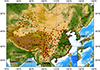 |
Figure 2 The geographical distribution of GNSS observation stations in China and its surrounding areas is provided by CMONOC (red circles) and MGEX (green circles). |
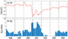 |
Figure 3 Geomagnetic indices were observed over 7 days from DOY 248 (September 5, 2017) to DOY 254 (September 11, 2017). |
From Figure 3, it can be observed that a geomagnetic storm commenced at 20:00 UT on DOY 250, leading to a sudden decrease in the Dst index. The Dst index reached its minimum value of −124 nT at 01:00 UT on DOY 251. During the periods from 00:00 UT to 03:00 UT and 13:00 UT to 15:00 UT on DOY 251, the Kp index reached its maximum value of 8. This indicates high-intensity geomagnetic activity, which may significantly affect technical infrastructure such as communication, navigation, and power systems in regions worldwide.
This paper adopts the root mean square error (RMSE) as the standard for evaluating assimilation results. The RMSE is defined as follows:
 (7)where M is the total number of assimilation points,
  represents the assimilated TEC obtained at the nth point, and
  represents the TEC value obtained by CODE or BDS GEO at the nth point. At the same time, four dynamic PPP modes are employed for accuracy assessment: ionosphere-free PPP (PPP/IF), CODE-based PPP (PPP/CODE), assimilated PPP (PPP/HBN), and IRI-based PPP (PPP/IRI). The reference coordinates are obtained from static dual-frequency PPP using the final solution (Zhou et al., 2018).
4 Single-station assimilation results and analysis
Before conducting regional assimilation modeling, it is essential to validate whether the HBN assimilation method can be effectively applied to data from a single station. Therefore, this study initially focuses on the assimilation of data from the JFNG station to assess the effectiveness and accuracy of the assimilation procedure in processing single-station data. Through the single-station assimilation experiment, we aim to ensure that the selected assimilation method can stably operate within a smaller research scope, thereby meeting the foundational requirement for extending the method to regional or global modeling. In this experiment, the TEC data from four MGEX BeiDou GEO satellites (C01–C04) were used, with IRI as the background model, and the HBN assimilation method was applied to the JFNG station. The experimental period was selected from DOY 248 to DOY 254, including quiet and disturbed ionospheric conditions.
In Figure 4, the black dots represent the GEO observation results, the blue line is the IRI model, and the red line denotes the HBN assimilation results. Due to differences in orbit and viewing geometry, the piercing points of satellites C01 to C04 vary, leading to slight differences in the TEC values computed at the same receiver site, JFNG.
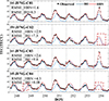 |
Figure 4 Single station assimilation experiment results. RMSE values for the IRI and HBN models are presented in TEC units (TECU). |
Figure 4 illustrates the comparison between the HBN assimilation results and GEO observations, further validating the effectiveness of the HBN method. Figure 4 also demonstrates that the RMSE of the HBN model is consistently lower than that of the IRI model, suggesting superior performance in TEC prediction. In single-station assimilation, the assimilation algorithm is highly dependent on the observation data, particularly the continuity of the data, which directly determines the quality of the assimilation results. As shown in Figures 4b and 4d, the red dashed boxes highlight significant gaps in the TEC data, resulting in large blank areas. Statistical analysis indicates that the missing data for C02 is primarily concentrated around DOY 254, which results in no significant errors in the assimilation values for C02 from DOY 248 to DOY 253. In contrast, the missing data for C04 is mainly concentrated around DOY 249 and DOY 254. Due to the missing data on DOY 249, C04 experiences a sharp increase in error, with an RMSE of 4.9 m on DOY 249. Additionally, C04 has a significant number of data gaps. After removing the continuous data gaps (DOY 249 and DOY 254), the missing data in C04 is approximately twice that of C01–C03. This results in the assimilation results for C04 relying more heavily on the background model, leading to a greater overall bias compared to C01–C03. The slight increase in errors for C02 and C03 may be attributed to satellite signal reception issues. The observation data for C01 exhibits slightly better smoothness compared to the other satellites.
However, when the observation data is relatively abundant and exhibits good continuity, the HBN assimilation method demonstrates strong assimilation capability.
Regardless of the disturbances, the predicted TEC values are generally close to the GEO observation results, with smaller errors overall. In summary, the HBN assimilation method shows promising effectiveness in single-station assimilation, particularly when the data is sufficient and of high quality, leading to a reduction in prediction errors.
5 Regional assimilation results and analysis
5.1 Under quiet ionospheric conditions
Figure 5 illustrates the ionospheric piercing point (IPP) TEC distribution for a quiet geomagnetic day (DOY 249, or September 6, 2017) at 05:00 UT in China and its surrounding areas. Figure 5 includes observations (IPP TEC), background model (IRI TEC), assimilated TEC, and CODE TEC. In the 130°E–140°E, 15°N–35°N region, the simulated values of IRI TEC are significantly larger than those of CODE TEC. In the 70°E–140°E, 35°N–55°N region, the simulated values of IRI TEC are notably lower than those of CODE TEC. The assimilated data through HBN shows better consistency with CODE TEC than the background IRI TEC. This indicates that, to some extent, the GNSS observational data, when assimilated with the HBN algorithm, exhibit significant improvement compared to the sole IRI model.
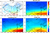 |
Figure 5 Comparison of IPP, IRI, assimilated, and CODE TEC values on DOY 249 (September 6, 2017) at 05:00 UT. The assimilation method employed is that of the HBN. |
The TEC values in the assimilated TEC map, particularly in the 130°E to 140°E, 15°N to 25°N regions are slightly higher than those in the CODE TEC map. Although these regions are predominantly oceanic and lack direct GNSS observations, the values remain within a reasonable range. In previous studies, similar conclusions were drawn using the LEnKF method, with assimilation values slightly higher than CODE values in oceanic regions (Tang et al., 2022). Statistical calculations in the region from 130°E to 140°E, 15°N to 25°N show that the RMSE between HBN and CODE is 9.3 TECU. However, considering the sparsity of GNSS stations in oceanic regions, CODE values tend to exhibit larger discrepancies from the true values. Therefore, we consider the HBN assimilation results to be within a reasonable range based on these comparative findings (Li et al., 2018; Suneetha et al., 2024). Unlike CODE TEC, which is a global TEC product primarily based on GNSS observations from densely distributed ground-based stations, HBN benefits from a model-based assimilation approach that incorporates broader prior information and physical constraints. The HBN model assumes spatial continuity in ionospheric conditions, meaning that TEC values in areas without direct data can be inferred from data in nearby regions. By combining neighboring data and background models, HBN produces more accurate TEC estimates, even in sparsely covered areas like oceans.
Figure 6 compares HBN TEC, KF TEC, and the background model IRI TEC against CODE TEC on DOY 249 (a geomagnetically quiet day). Figure 6a–6c presents the residual histograms, and Figure 6d–6f shows scatter plots, all using CODE TEC as the reference truth. The HBN algorithm demonstrates superior performance, with a residual mean of −1.00 TECU and an RMSE of 3.65 TECU, indicating a closer alignment with CODE TEC. In contrast, the KF model has a residual mean of −3.4 TECU and an RMSE of 4.12 TECU, while the IRI model shows a residual mean of −3.33 TECU and an RMSE of 5.20 TECU. While the residuals of HBN are not perfectly centered around zero, as shown in Figure 6a, they are more tightly clustered and closer to zero than the KF and IRI models. This indicates that, despite a slight bias, the HBN approach still exhibits significantly reduced errors. Incorporating HBN assimilation reduced the RMSE by 29.8% compared to the IRI model, while the KF model reduced the RMSE by only 20.7%.
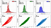 |
Figure 6 On DOY 249 (September 6, 2017), residual histograms and scatter plots compare HBN TEC, KF TEC, and IRI TEC against CODE TEC. Black solid lines in (a)–(c) indicate a mean of zero, while in (d)–(f), they represent linear regression lines, reflecting the relationship between model estimates and CODE TEC values. Note: “KF” refers to the Kalman Filter-based method for TEC estimation. |
The correlation coefficient R quantifies the strength and direction of a linear relationship between two variables. The scatter plot for HBN TEC in Figure 6d demonstrates a high correlation coefficient R = 0.95 with CODE TEC, with data points closely aligning along the y = x line, indicative of excellent predictive accuracy. In contrast, Figure 6e shows the KF models exhibiting slightly higher correlation coefficients of R = 0.96. However, the KF and the IRI residual distributions are less centralized, reflecting more significant inconsistency and error. The assimilated TEC after the HBN algorithm provides a more accurate fit to the IRI model. The model performance is significantly improved, aligning more with actual data and exhibiting greater consistency with CODE TEC. The accuracy of the HBN assimilation model is superior to that of the KF and IRI models. However, the scatter points for HBN exhibit greater dispersion than those of IRI and KF. This may be attributed to the fact that both KF and IRI tend to smooth the data, adopting a more conservative approach to handling variations, resulting in less scatter. In contrast, the HBN model, with its more flexible assimilation process, is capable of capturing finer variations in ionospheric TEC. Consequently, when CODE TEC data exhibits rapid changes or localized anomalies, the HBN model is more likely to reflect these details, leading to a relatively more dispersed distribution of scatter points. Additionally, it is important to note that CODE TEC is not perfectly accurate, as it is derived from interpolation of GNSS observations, particularly in regions with sparse receiver coverage, such as oceans. This inherent limitation in CODE TEC can introduce uncertainties, which may also contribute to the observed scatter.
To assess the accuracy of assimilating HBN TEC models, this paper employs four dynamic PPP modes: PPP/IF, PPP/CODE, PPP/HBN, and PPP/IRI. Figure 7 illustrates the 3D coordinate RMSE for each epoch at four MGEX GEO stations on DOY 249 (September 6, 2017) under the four modes. These stations were not involved in constructing the HBN model. They were used exclusively for validation. TEC values for PPP/CODE, PPP/HBN, and PPP/IRI were obtained from global CODE TEC, CMONOC TEC processed by HBN assimilation, and IRI-2016, respectively. The PPP/IF method used dual-frequency observations without relying on external TEC data. The RMSE for 3D coordinates (North, East, and Up) is computed based on the solution for these coordinates. PPP/HBN is based on single-frequency observations for PPP with ionospheric assimilated TEC. PPP/IF serves as a reference for accuracy. If the positioning accuracy of single-frequency PPP with ionospheric constraints is slightly lower than or equal to PPP/IF, it can be demonstrated that ionospheric TEC is more accurate.
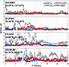 |
Figure 7 RMSE (in meters) of 3D positioning errors across epochs at different stations on DOY 249 (September 6, 2017): (a) GAMG, (b) JFNG, (c) LHAZ, (d) CMUM. |
It can be observed that both PPP/HBN and PPP/CODE solutions exhibit good performance for all stations, similar to PPP/IF. The PPP/IRI model exhibits particularly significant errors, with highly fluctuating error patterns. This can be attributed to the inherent limitations of the IRI model as an empirical model, which has an upper altitude limit for its calculations. Therefore, the computed TEC may differ from actual observations. A comparison between the pre-assimilation (PPP/IRI) and post-assimilation (PPP/HBN) models highlights the effectiveness of HBN assimilation in reducing positioning errors.
From Figure 7a GAMG, it can be observed that at UT 8, the overall error of PPP/IRI is relatively tiny. This is because IRI, as an empirical model, is suitable for conditions where the ionosphere is relatively stable, thus providing a more accurate ionospheric delay correction during this time period. On the other hand, the PPP/HBN method may be affected by the uneven distribution of the ionosphere locally or the precision of real-time correction products, leading to a slight increase in error at UT 8.
The results indicate that ionospheric constraints in PPP/HBN can effectively enhance single-frequency PPP positioning. In Figure 7d, TEC values are higher in low-latitude regions due to increased ionospheric activity, leading to generally poorer performance for all PPP methods. The results of the positioning analysis demonstrate that HBN, through the integration of multi-source observational data and a priori modeling, exhibits high temporal and spatial resolution and is capable of providing reliable ionospheric electron density predictions under diverse conditions. This result serves to demonstrate the rationality and superiority of the revised algorithm.
5.2 Under disturbed ionospheric conditions
Figure 8 illustrates the ionospheric TEC distribution in China and surrounding regions during a geomagnetic storm day (DOY 251, or September 8, 2017) at 05:00 UT, including IPP TEC, background model IRI TEC, assimilated TEC, and CODE TEC. In the 70°E–140°E, 15°N–35°N region, the simulated values of IRI TEC are noticeably lower than those of CODE TEC. After HBN assimilation, the assimilated TEC shows greater consistency with CODE TEC than the background IRI TEC. To some extent, this indicates that after GNSS observations of TEC data undergo HBN assimilation into the IRI model on disturbed days, the IRI model has been improved and is more in line with the objective observational data from IPP, demonstrating increased practical utility.
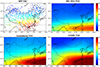 |
Figure 8 Comparison of IPP, IRI, assimilated, and CODE TEC values on DOY 251 (September 8, 2017) at 05:00 UT. The assimilation method employed is that of the HBN. |
Figure 9 depicts the histogram of residuals and scatter distribution for HBN TEC, KF TEC, and the background model IRI on the disturbance day, using CODE TEC as the true value. The residual histograms and scatter plots for HBN TEC, KF TEC, and IRI TEC demonstrate that HBN TEC has the lowest mean residual of −1.11 TECU and RMSE of 3.80 TECU, indicating high consistency with CODE TEC. In contrast, KF TEC shows a mean residual of −2.64 TECU and an RMSE of 4.30 TECU. IRI TEC exhibits a mean residual of −5.56 TECU and an RMSE of 7.52 TECU, indicating larger discrepancies. The scatter plots further confirm these findings, with HBN TEC showing the highest correlation coefficient of 0.95, followed by KF TEC at 0.94 and IRI TEC at 0.90. This study indicates that data assimilation effectively integrates GNSS-based observational data into the background model, resulting in more reasonable and accurate ionospheric TEC outcomes.
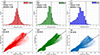 |
Figure 9 On DOY 251 (September 8, 2017), residual histograms and scatter plots compare HBN TEC, KF TEC, and IRI TEC against CODE TEC. Black solid lines in (a)–(c) indicate a mean of zero, while in (d)–(f), they represent linear regression lines, reflecting the relationship between model estimates and CODE TEC values. |
The results show that the KF method achieves lower average biases during ionospheric disturbance periods (−2.64) compared to quiet periods (−3.4). This seemingly counterintuitive result can be explained by the adaptive nature of the KF method (Mungufeni et al., 2022; Qiao et al., 2022). During ionospheric disturbances, the variability in the TEC increases, which leads to larger fluctuations in GNSS observations. The KF method dynamically adjusts its estimates based on these real-time fluctuations, allowing it to more effectively capture the rapid changes in TEC, thus aligning more closely with the CODE-derived TEC under disturbed conditions (Manin et al., 2021; Kosary et al., 2022). Conversely, during quiet periods, when the ionospheric conditions are relatively stable, the KF’s smoothing process, which relies on the assumption of a relatively constant signal, may result in slightly higher biases due to the over-smoothing of the already stable TEC values. This over-smoothing effect is a known issue in Kalman filtering when applied to systems with little variation, as it can lead to an underestimation of the true noise level and introduce small errors (Anghel et al., 2009; Sætrøm and Omre, 2011).
Figure 10 illustrates the 3D RMSE values of the four modes at different stations for each epoch on the disturbed day. The PPP/HBN and PPP/CODE schemes perform well at all sites, as does PPP/IF. Due to ionospheric disturbances, PPP/IRI exhibits larger errors and more significant fluctuations compared to geomagnetically quiet days. The results also indicate that the ionospheric constraints of PPP/HBN are effective for single-frequency PPP localization under disturbed ionospheric conditions. Similar to Figure 7, the performance of all PPP methods in Figure 10d is generally poor. Jiang et al. (2020) demonstrated that ionospheric irregularities were present in low-latitude Southeast Asia on September 8, 2017, at approximately 13:00 UT. Additionally, a significant error is present around 01:00 UT and from 13:00 UT to 16:00 UT, when ionospheric irregularities significantly affect GNSS observations.
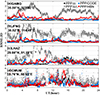 |
Figure 10 RMSE (in meters) of 3D positioning errors across epochs at different stations on DOY 251 (September 8, 2017): (a) GAMG, (b) JFNG, (c) LHAZ, (d) CMUM. |
Between 4 and 10 September 2017, significant solar eruptions originating from active region AR12673 triggered impactful space weather events observed from the Sun to the Earth’s magnetosphere. These events were meticulously recorded by the National Oceanic and Atmospheric Administration and National Aeronautics and Space Administration spacecraft, with the September 6 X9.3 flare, occurring at 11:53 UT, being the largest of solar cycle 24 and the brightest since the X17 flare of September 2005 in solar cycle 23. The associated coronal mass ejection, launched at 12:12 UT on September 6, traversed the interplanetary medium and arrived at Earth on September 7. This coronal mass ejection induced a series of geomagnetic storms, with two peaks on September 8 at approximately 01:00 UT and 14:00 UT, corresponding to Dst minimum values of −142 nT and −124 nT, respectively, marking the culmination of intense geomagnetic activity (Schillings et al., 2018; Blagoveshchensky et al., 2019; Werner et al., 2019; Owolabi et al., 2020).
Given these space weather events, particularly the solar flare and associated coronal mass ejection, the ionosphere was likely disturbed on September 6, which may have influenced the results from this day. While geomagnetic conditions suggest some degree of quietness, the solar flare activity on September 6 caused ionospheric disturbances during the flare period.
Such geomagnetic disturbances can significantly influence the Earth’s ionosphere, giving rise to ionospheric irregularities that induce amplitude and phase scintillation in GNSS signals. These effects are particularly detrimental to PPP solutions, where the accuracy of PPP/IF, PPP/CODE, and PPP/HBN methods is adversely affected. Even though the first-order ionospheric delay is corrected in PPP/IF, it may still fall short of mitigating the full impact of scintillation on GNSS signal quality.
6 Discussion
As shown in Figure 11, to verify the reliability of the HBN assimilation algorithm, we selected four GNSS stations not involved in the ionospheric modeling: GAMA-C01, JFNG-C01, LHAZ-C01, and CMUM-C01. These stations were used for assimilation experiments and accuracy assessment. The TEC values from GNSS observations (black), the IRI model (blue), the KF assimilation (green), and the HBN assimilation (red) were compared. Since the IPP of BDS GEO satellites remains relatively fixed, the TEC variations at specific locations can be analyzed continually over an extended period. Thus, the TEC derived from the GEO satellites served as a reference to assess the accuracy of the assimilation results. To ensure consistency across the models, TEC values for all methods (KF, HBN, and IRI) were interpolated to the station locations, as the KF and HBN model outputs were provided at a 1° × 1° resolution. While we also computed KF and HBN using higher-resolution models (0.5° × 0.5°), the computational cost was considerably higher, and the results showed no significant difference compared to the 1° × 1° resolution. Similarly, directly calculating TEC values from the IRI model at the stations produced results comparable to those of the interpolation method. Therefore, in the interest of consistency and computational efficiency, we chose to use the 1° × 1° models and interpolate TEC values to the station locations. These interpolated values were then compared with the TEC derived from the GEO satellites. As shown in Figure 11, the HBN assimilation algorithm demonstrates superior prediction accuracy, with the predicted values (red line) closely matching the observed values (black dots) at all sites. In particular, the results at JFNG-C01 and CMUM-C01 show a notable consistency between the HBN predictions and observations.
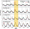 |
Figure 11 Comparison of TEC values over 7 days from DOY 248 to 254 (September 5–11, 2017) using data from GNSS observations (black), the IRI model (blue), the KF assimilation (green), and the HBN assimilation (red) at different stations. |
During the significantly disturbed day (DOY 251, or September 8, 2017), characterized by strong geomagnetic activity (KPmax = 8), the TEC derived from GEO satellites was used as the reference. The HBN method achieved an RMSE of 9.2 TECU, representing a notable improvement over the KF method, which had an RMSE of 10.9 TECU. This highlights the capability of HBN to more effectively capture ionospheric TEC variations under extreme disturbance conditions.
The HBN assimilation algorithm generally outperforms the IRI and KF models across all sites and periods. Notably, under conditions of significant ionospheric variability, HBN more accurately captures the underlying trends than the other models. This demonstrates the effectiveness of the HBN method in leveraging observational data to enhance TEC prediction accuracy, providing more reliable support for space weather monitoring, navigation, and communication systems.
Nevertheless, we acknowledge that accurately modeling the positive storm effect remains inherently challenging. While our assimilation method has demonstrated success in capturing ionospheric disturbances overall, it may not fully account for the complexities associated with the positive storm effect, especially during periods of intense geomagnetic activity. In particular, short-term phenomena such as TEC enhancements and depressions during severe storm conditions may not be sufficiently captured by the model, as highlighted in the red-boxed period in Figure 11 and reported in previous studies (Uwamahoro & Habarulema, 2015; Bruinsma et al., 2021). This limitation should be taken into account when interpreting the model’s performance under extreme ionospheric conditions.
Figure 12 shows a comparison between regional modeling and single-station modeling for JFNG-C01. Figure 12b shows the TEC values interpolated to the JFNG coordinates after regional modeling using CMONOC observation data.
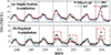 |
Figure 12 Comparison between single-station modeling and regional modeling for JFNG-C01. |
Both methods use the HBN assimilation with the IRI model as the background. Using GEO TEC as the reference, the RMSE of single-station modeling is 1.6 TECU, while the regional assimilation error is 8.2 TECU. Since JFNG data is not used in regional modeling, the regional model inevitably has more significant errors than the single-station model. The regional models face more difficulties in constraining ionospheric variations compared to single-station models. The larger the region modeled, the more challenging it becomes to represent local ionospheric features accurately. This is particularly true when considering global models or during periods of intense ionospheric disturbances such as magnetic storms. As regional models attempt to capture the variation of ionospheric parameters over a larger area, they may face challenges in accurately modeling local disturbances, thus leading to greater uncertainties when compared to single-station models.
During magnetic storm periods, regional models tend to fail to capture the positive storm effects. This is mainly because regional models rely on interpolated or weighted data from multiple stations, which can introduce errors, especially in regions with sparse data or during significant ionospheric disturbances. In contrast, single-station models, by directly assimilating data from a single observation point, are better at capturing local variations and ionospheric perturbations, including the positive storm effects. It is important to note that regional models perform relatively well when the ionosphere is “quiet” and disturbances are minimal, as the background model provides sufficient accuracy in such cases.
Several studies have shown that regional models often struggle to capture the positive storm effects, especially when ionospheric disturbances are strong (Uwamahoro & Habarulema, 2015; Bruinsma et al., 2021). The reliance on background models and interpolation techniques in regions with sparse data can exacerbate the inaccuracies during such periods.
However, unlike single-station modeling, which relies on data from a single observation point, HBN regional modeling integrates data from multiple stations, providing more comprehensive ionospheric information and reducing the limitations of single-station data. The HBN model assumes spatial continuity in ionospheric conditions, meaning that TEC values in areas without direct data can be inferred from data in nearby regions. In areas without data, the regional assimilation technique in the HBN model uses a combination of neighboring station data and background models. While the HBN model significantly reduces the impact of the background model compared to single-station modeling, it still tends to rely on background data to some extent in areas with sparse coverage, leading to a certain degree of bias toward the background model. While both methods may approach the background model in the absence of data, the HBN regional modeling’s use of multiple stations and spatial continuity assumption provides additional information, leading to more stable and accurate assimilation results, even in sparsely covered areas like oceans.
To assess the accuracy of the assimilated results, Figure 13 displays the RMSE of the 3D coordinates for different stations from DOY 248 to 254. The RMSE of the 3D coordinates for all selected stations gradually increases with decreasing latitude. The positioning accuracy of the PPP/Assimilated method is usually slightly lower than that of the PPP/CODE method for the GAMG and CMUM stations. Based on the distribution of GNSS stations in Figure 2, the lower accuracy in the assimilation of ionospheric data around the GAMG and CMUM stations may have contributed to the reduced accuracy of PPP/Assimilated positioning. However, the PPP/Assimilated method generally provides higher positioning accuracy than the PPP/CODE method for the JFNG and LHAZ stations.
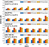 |
Figure 13 RMSE of 3D positioning with each day at different stations from September 5, 2017, to September 11, 2017. (a) GAMG; (b) JFNG; (c) LHAZ; (d) CMUM. The blue bar represents PPP/IF, the red bar represents PPP/CODE, and the yellow bar represents PPP/Assimilated using the assimilation method HBN. Shorter bars indicate a reduction in localization errors. |
Additionally, more GNSS stations near the JFNG and LHAZ stations contribute to the ionospheric assimilation model, indicating greater accuracy of the assimilated ionospheric model in this area. Figure 13 demonstrates that the assimilated ionospheric model enhances accuracy in this region. The assimilated TEC improves the accuracy of 3D coordinates in areas where more stations are involved in the assimilation. However, the assimilated TEC exhibits reduced accuracy in areas with fewer stations involved in the assimilation.
The results of the PPP/IF methods demonstrate effective mitigation of almost all errors. However, in Figure 13d, the performance of the four PPP methods is notably worse on the disturbed DOY 251. As analyzed in Figure 10, scintillation caused by ionospheric irregularities may be the main reason for the poor PPP/IF results, and both PPP/CODE and PPP/Assimilated exhibit poor results on the disturbed day. Jiang et al. (2020) reported significant ionospheric scintillation in Southeast Asia on disturbed days at low latitudes. The statistical results indicate that the PPP/Assimilated method slightly outperforms PPP/CODE in improving GNSS positioning accuracy. From DOY 248 to 254, the average RMSE of PPP/Assimilated was 0.52 m, compared to 0.58 m for PPP/CODE. In TEC prediction, HBN significantly outperforms CODE; however, it only slightly surpasses CODE in GNSS positioning. HBN incorporates a broader range of observational data and prior physical models, enhancing TEC accuracy. However, GNSS positioning accuracy is not solely dependent on TEC precision; it is also influenced by factors such as multi-path effects, geometric dilution of precision, satellite orbit errors, and receiver biases.
Table 1 presents the RMSE, correlation coefficient, and average absolute percentage deviation (AAPD) values during assimilation (DOY 244–273) at stations GAMA, JFNG, LHAZ, and CMUM to assess the HBN assimilation performance at these four stations. The comprehensive evaluation using these three metrics provides a holistic assessment of the assimilation results, reflecting their accuracy, bias, and trend-fitting capability (Forootan et al., 2023). We selected a longer period (DOY 244–273) to evaluate the model’s overall performance under varying ionospheric conditions, including both geomagnetically disturbed and quiet periods. This extended time frame provides a more comprehensive assessment of the HBN method’s performance, particularly its reliability over long-term datasets. The experimental true value is based on BDS GEO observations. Furthermore, to facilitate a side-by-side comparison of the HBN algorithms, the assimilation effect of the KF for the same experiment is presented in Table 1.
Summary of RMSE, R, and AAPD measures for assessing HBN assimilation performance at four MGEX stations (DOY 244–273, September 1–30, 2017).
The RMSE analysis reveals significant improvements for both the KF and HBN methods compared to the IRI model, with reductions of 20.17% and 33.14%, respectively. Among the evaluated sites, the CMUM station exhibited the greatest RMSE reduction, where the HBN method achieved a reduction of 45.02%, outperforming the KF method’s 34.26% reduction. These results highlight the effectiveness of the assimilation algorithms, particularly the HBN method, in correcting TEC values at low latitudes. The superior performance of HBN can be attributed to its ability to integrate additional observational data and prior physical constraints, which enhances its accuracy in regions with complex ionospheric conditions. This trend suggests that HBN is more adept at capturing TEC variations under low-latitude conditions than KF. Further statistical validation could provide additional insights into the robustness of these results.
The correlation coefficients obtained from the HBN model are consistently higher than those of the KF and IRI models across all sites, demonstrating its superior performance in ionospheric TEC assimilation. Notably, at the JFNG and LHAZ sites, the correlation coefficient values for the HBN model approach are close to 1.00, indicating an exceptional predictive capability. In comparison, while the IRI model achieves relatively high correlation coefficient values at most sites, it falls short of matching the accuracy of the HBN model. The KF model, on the other hand, exhibits the lowest correlation coefficient values among the three methods across all sites.
The poor correlation coefficient performance of the KF model compared to the IRI model can be attributed to its inherent assumptions. The KF algorithm assumes linear system dynamics and Gaussian distributions for both process and observational noise, which limits its ability to accurately capture the highly nonlinear and spatially complex nature of ionospheric electron density distributions. This limitation leads to biases in the assimilation results, adversely affecting the correlation coefficients. In contrast, the HBN model effectively incorporates prior information and observational data into a Bayesian framework, enabling it to account for non-linear effects and better align with the true ionospheric state. These results suggest that the HBN approach is better suited for TEC assimilation under dynamic ionospheric conditions.
AAPD is expressed as the percentage of the absolute difference between observation and model, as has been widely used in previous studies of model evaluation, particularly in ionospheric and atmospheric modeling (Bruinsma et al., 2021):
 (8)
(8)
The AAPD provides a straightforward metric for evaluating the predictive performance of models, with lower values indicating smaller deviations from observed values (Forootan et al., 2023). Table 1 shows that the HBN algorithm consistently achieves lower AAPD values than the KF and IRI models across all GNSS stations, reflecting its superior predictive accuracy. Notably, at the CMUM station (low latitude), the AAPD of HBN is 0.25, significantly better than the IRI model’s 0.48, demonstrating HBN’s ability to correct TEC values under dynamic ionospheric conditions effectively.
The HBN model demonstrates superior performance in TEC modeling, as evidenced by the consistently lower RMSE and AAPD values compared to the IRI reference model and KF. The smaller RMSE indicates that the HBN model achieves higher prediction accuracy, while the AAPD results underscore its ability to minimize percentage deviations across diverse conditions. Notably, the correlation coefficients for HBN exceed those of KF and IRI at all sites, further validating the model’s ability to produce precise and reliable TEC predictions. While the HBN model outperforms KF and IRI, the results also highlight challenges in regions with sparse observations or during periods of severe ionospheric disturbances, such as DOY 251. These findings confirm that the HBN assimilation method provides a robust framework for establishing accurate TEC models under varied ionospheric conditions.
Although the HBN model demonstrated excellent performance in TEC prediction throughout September, particularly in low-latitude regions, this does not imply that GNSS positioning accuracy was equally high across all periods. While accurate TEC predictions contribute to improved ionospheric modeling, GNSS positioning accuracy is influenced by additional factors, particularly during ionospheric disturbance days, when positioning accuracy is significantly affected by ionospheric scintillation.
As shown in Table 2, the statistical results of this study indicate a significant difference in model performance between day and night. During the period from DOY 244 to 273, we observed that the model’s accuracy was higher during the day, while there was a noticeable decrease in accuracy at night. This trend is evident not only in the HBN method but also in the results of the KF method. This further highlights the impact of ionospheric fluctuations and the time period on data assimilation accuracy.
RMSE comparison of HBN and KF models for different time periods (DOY 244–273, September 1–30, 2017).
At the same time, we observed that the difference in assimilation accuracy between day and night in the HBN method was much smaller than in the KF method. This suggests that the HBN method exhibits greater adaptability across different time periods, providing more stable results under various ionospheric conditions.
7 Conclusion
This work employs the HBN assimilation method with IRI as the background model, using observational data provided by CMONOC from approximately 260 ground-based GNSS stations. An HBN assimilation model for China and its surrounding regions 15°N–55°N, 70°E–140°E is established. The TEC data from BDS GEO and CODE TEC are used to evaluate the assimilation effectiveness of HBN on the ionospheric TEC from DOY 244 to 273 of the year 2017. A KF model is built using the same data to compare the HBN assimilation effects side-by-side. Finally, this work uses the PPP approach to evaluate the practical application value of the HBN assimilation calculation algorithm.
By analyzing the experimental results during both quiet and disturbed geomagnetic conditions, it can be concluded that the HBN algorithm effectively improves the accuracy of ionospheric TEC regardless of geomagnetic activity. The experiment demonstrated that HBN outperforms the KF algorithm. Statistical assimilation results show that the correlation coefficient is, on average, improved by approximately 14%, and the RMSE is reduced by approximately 33% for HBN compared to IRI, using the BDS GEO satellite IPP as the reference. Furthermore, each index shows a notable improvement in performance compared to the KF algorithm. HBN assimilation is particularly effective at lower latitudes. However, the results of the HBN model during peak times of magnetic storms still differ somewhat from the observed values at individual stations, which may be due to the excessive intensity of the magnetic storms.
Moreover, evaluating the performance of HBN using the PPP method shows that incorporating ionospheric constraints in PPP/Assimilated can significantly enhance the accuracy of single-frequency PPP. Even on disturbed days, eliminating the first-order ionospheric delay in PPP/IF is insufficient to mitigate the impact of scintillation on the GNSS signal. Ionospheric irregularities may cause scintillation, which could be the main reason for the poor results obtained from the PPP/IF, PPP/CODE, and PPP/Assimilated methods (Priyadarshi, 2015). The HBN method can therefore be considered a valuable tool for data assimilation in spatial environmental monitoring, navigation, and positioning applications.
Acknowledgments
The authors thank the GNSS Center at Wuhan University for providing the GNSS observation data of the Crustal Movement Observation Network of China (CMONOC). We thank the anonymous referees and the editor for their helpful comments and suggestions. The editor thanks Marjolijn Adolfs and John Bosco Habarulema for their assistance in evaluating this paper.
Funding
This work was supported by the National Natural Science Foundation of China (42261074) and the Yunnan Fundamental Research Projects (202401AS070067, 202501AS070106).
Conflicts of interest
The authors declare no conflict of interest.
Data availability statement
MGEX data are available from https://cddis.nasa.gov/archive/gnss/data/campaign/mgex/. CODE global ionospheric map products are obtained from the Center for Orbit Determination in Europe data repository (ftp://ftp.aiub.unibe.ch/CODE/). The IRI-2016 data can be downloaded from the IRI official website (http://www.irimodel.org). The GSFC/SPDF OmniWeb provides the geomagnetic and solar activity data (http://omniweb.gsfc.nasa.gov).
References
- Aa E, Huang W, Yu S, Liu S, Shi L, et al. 2015. A regional ionospheric TEC mapping technique over China and adjacent areas on the basis of data assimilation. J Geophys Res Space Phys 120(6): 5049–5061. https://doi.org/10.1002/2015JA021140. [CrossRef] [Google Scholar]
- Anghel A, Carrano C, Komjathy A, Astilean A, Letia T. 2009. Kalman filter-based algorithms for monitoring the ionosphere and plasmasphere with GPS in near-real time. J Atmos Sol Terr Phys 71(1): 158–174. https://doi.org/10.1016/j.jastp.2008.10.006. [CrossRef] [Google Scholar]
- An X, Meng X, Chen H, Jiang W, Xi R, et al. 2020. Modelling global ionosphere based on multi-frequency, multi-constellation GNSS observations and IRI model. Remote Sens 12(3): 439. https://doi.org/10.3390/rs12030439. [CrossRef] [Google Scholar]
- Banerjee S, Carlin BP, Gelfand AE. 2003. Hierarchical modeling and analysis for spatial data, Chapman and Hall/CRC, New York, NY. https://doi.org/10.1201/9780203487808. [CrossRef] [Google Scholar]
- Blagoveshchensky DV, Sergeeva MA, Corona-Romero P. 2019. Features of the magnetic disturbance on September 7–8, 2017 by geophysical data. Adv Space Res, 64(1): 171–182. https://doi.org/10.1016/j.asr.2019.03.037. [CrossRef] [Google Scholar]
- Bruinsma S, Boniface C, Sutton EK, Fedrizzi M. 2021. Thermosphere modeling capabilities assessment: geomagnetic storms. J Space Weather Space Clim 11: 12. https://doi.org/10.1051/swsc/2021002. [CrossRef] [EDP Sciences] [Google Scholar]
- Carlin BP, Banerjee S. 2003. Hierarchical multivariate CAR models for spatio-temporally correlated survival data. Bayesian Statistics 7(7): 45–63. [Google Scholar]
- Chen M, Liu L, Xu C, Wang Y. 2020. Improved IRI-2016 model based on BeiDou GEO TEC ingestion across China. GPS Solut 24: 20. https://doi.org/10.1007/s10291-019-0938-8. [CrossRef] [Google Scholar]
- Forootan E, Farzaneh S, Kosary M, Schmidt M, Schumacher M. 2021. A simultaneous calibration and data assimilation (C/DA) to improve NRLMSISE00 using thermospheric neutral density (TND) from space-borne accelerometer measurements. Geophys J Int 224(2): 1096–1115. https://doi.org/10.1093/gji/ggaa507. [Google Scholar]
- Forootan E, Kosary M, Farzaneh S, Schumacher M. 2023. Empirical data assimilation for merging total electron content data with empirical and physical models. Surv Geophys 44(6): 2011–2041. https://doi.org/10.1007/s10712-023-09788-7. [CrossRef] [Google Scholar]
- Fuller-Rowell T, Araujo-Pradere E, Minter C, Codrescu M, Spencer P, et al. 2006. US-TEC: A new data assimilation product from the Space Environment Center characterizing the ionospheric total electron content using real-time GPS data. Radio Sci 41(6): RS6003. https://doi.org/10.1029/2005RS003393. [CrossRef] [Google Scholar]
- Gardner CL, Schunk RW, Scherliess L, Sojka JJ, Zhu L. 2014. Global Assimilation of Ionospheric Measurements-Gauss Markov model: improved specifications with multiple data types. Space Weather 12(12): 675–688. https://doi.org/10.1002/2014SW001104. [CrossRef] [Google Scholar]
- Grynyshyna-Poliuga O. 2024. Simultaneous monitoring of the limited area ionosphere with the use of GPS and ionosonde. Adv Space Res 73(12); 5964–5977. https://doi.org/10.1016/j.asr.2024.03.003. [CrossRef] [Google Scholar]
- Gu S, Dai C, Fang W, Zheng F, Wang Y, et al. 2021. Multi-GNSS PPP/INS tightly coupled integration with atmospheric augmentation and its application in urban vehicle navigation. J Geod 95(6): 64. https://doi.org/10.1007/s00190-021-01514-8. [CrossRef] [Google Scholar]
- Hajj GA, Wilson BD, Wang C, Pi X, Rosen IG 2004. Data assimilation of ground GPS total electron content into a physics-based ionospheric model by use of the Kalman filter. Radio Sci 39(1): RS1S05. https://doi.org/10.1029/2002RS002859. [Google Scholar]
- Jiang C, Wei L, Yang G, Aa E, Lan T, et al. 2020. Large-scale ionospheric irregularities detected by ionosonde and GNSS receiver network. IEEE Geosci Remote Sens Lett 18(6): 940–943. https://doi.org/10.1109/LGRS.2020.2990940. [Google Scholar]
- Kosary M, Forootan E, Farzaneh S, Schumacher M. 2022. A sequential calibration approach based on the ensemble Kalman filter (C-EnKF) for forecasting total electron content (TEC). J Geod 96(4): 29. https://doi.org/10.1007/s00190-022-01623-y. [CrossRef] [Google Scholar]
- Li M, Yuan Y, Wang N, Li Z, Huo X. 2018. Performance of various predicted GNSS global ionospheric maps relative to GPS and JASON TEC data. GPS Solut 22, 55. https://doi.org/10.1007/s10291-018-0721-2. [CrossRef] [Google Scholar]
- Lin CY, Matsuo T, Liu JY, Lin CH, Huba JD, et al. 2017. Data assimilation of ground-based GPS and radio occultation total electron content for global ionospheric specification. J Geophys Res Space Phys 122(10): 10876–10886. https://doi.org/10.1002/2017JA024185. [Google Scholar]
- Mao T, Wan W, Yue X, Sun L, Zhao B, et al. 2008. An empirical orthogonal function model of total electron content over China. Radio Sci 43(2): RS2009. https://doi.org/10.1029/2007RS003629. [Google Scholar]
- Manin AA, Sokolov SV, Novikov AI, Polyakova MV, Demidov DN, et al. 2021. Kalman filter adaptation to disturbances of the observer’s parameters. Inventions 6(4): 80. https://doi.org/10.3390/inventions6040080. [CrossRef] [Google Scholar]
- McMillan NJ, Holland DM, Morara M, Feng J. 2010. Combining numerical model output and particulate data using Bayesian space-time modeling. Environmetrics 21(1): 48–65. https://doi.org/10.1002/env.984. [CrossRef] [Google Scholar]
- Mukhtaro P, Pancheva D, Andonov B, Pashova L. 2013. Global TEC maps based on GNSS data: 1. Empirical background TEC model. J Geophys Res Space Phys 118(7): 4594–4608. https://doi.org/10.1002/jgra.50413. [CrossRef] [Google Scholar]
- Mungufeni P, Migoya-Orué Y, Matamba TM, Omondi G. 2022. Application of classical Kalman filtering technique in assimilation of multiple data types to NeQuick model. J Space Weather Space Clim 12: 9. https://doi.org/10.1051/swsc/2022006. [CrossRef] [EDP Sciences] [Google Scholar]
- Owolabi C, Lei J, Bolaji OS, Ren D, Yoshikawa A. 2020. Ionospheric current variations induced by the solar flares of 6 and 10 September 2017. Space Weather 18(11): e2020SW002608. https://doi.org/10.1029/2020SW002608. [CrossRef] [Google Scholar]
- Peng J, Yuan Y, Liu Y, Zhang H, Zhang T, et al. 2024. Evaluation of GNSS-TEC data-drive IRI-2016 model for electron density. Atmosphere 15(8): 958. https://doi.org/10.3390/atmos15080958. [CrossRef] [Google Scholar]
- Priyadarshi S. 2015. A review of ionospheric scintillation models. Surv Geophys 36: 295–324. https://doi.org/10.1007/s10712-015-9319-1. [CrossRef] [Google Scholar]
- Qiao J, Liu Y, Fan Z, Tang Q, Li X, et al. 2021. Ionospheric TEC data assimilation based on Gauss-Markov Kalman filter. Adv Space Res 68(10): 4189–4204. https://doi.org/10.1016/j.asr.2021.08.004. [CrossRef] [Google Scholar]
- Qiao J, Zhou C, Liu Y, Zhao J, Zhao Z. 2022. Ionospheric Kalman filter assimilation based on covariance localization technique. Remote Sens 14(16): 4003. https://doi.org/10.3390/rs14164003. [CrossRef] [Google Scholar]
- Qin J, Liang S, Yang K, Kaihotsu I, Liu R, et al. 2009. Simultaneous estimation of both soil moisture and model parameters using particle filtering method through the assimilation of microwave signal. J Geophys Res Atmos 114(D15): D15103. https://doi.org/10.1029/2008JD011358. [Google Scholar]
- Rayner P. 2020. Data assimilation using an ensemble of models: a hierarchical approach. Atmos Chem Phys 20(6): 3725–3737. https://doi.org/10.5194/acp-20-3725-2020. [CrossRef] [Google Scholar]
- Ren X, Zhang X, Schmidt M, Zhao Z, Chen J, et al. 2020. Performance of GNSS global ionospheric modeling augmented by LEO constellation. Earth Space Sci 7(1): e2019EA000898. https://doi.org/10.1029/2019EA000898. [CrossRef] [Google Scholar]
- Schillings A, Nilsson H, Slapak R, Wintoft P, Yamauchi M, et al. 2018. O+ escape during the extreme space weather event of 4–10 September 2017. Space Weather 16(9): 1363–1376. https://doi.org/10.1029/2018SW001881. [CrossRef] [Google Scholar]
- Schunk RW, Scherliess L, Sojka JJ, Thompson DC, Anderson DN, et al. 2004. Global assimilation of ionospheric measurements (GAIM). Radio Sci 39(1): RS1S02. https://doi.org/10.1029/2002RS002794. [Google Scholar]
- Song JJ, Mallick B. 2019. Hierarchical Bayesian models for predicting spatially correlated curves. Statistics 53(1): 196–209. https://doi.org/10.1080/02331888.2018.1547905. [CrossRef] [Google Scholar]
- Ssessanga N, Kim YH, Habarulema JB, Kwak YS. 2019. On imaging South African regional ionosphere using 4D-var technique. Space Weather 17(11): 1584–1604. https://doi.org/10.1029/2019SW002321. [CrossRef] [Google Scholar]
- Suneetha E, Ratnam DV, Leong TE. 2024. Regional ionospheric TEC modeling during geomagnetic storm in August 2021 – data fusion using multi-instrument observations. Adv Space Res 73(7): 3818–3832. https://doi.org/10.1016/j.asr.2023.06.054. [CrossRef] [Google Scholar]
- Sætrøm J, Omre H. 2011. Ensemble Kalman filtering with shrinkage regression techniques. Comput Geosci 15: 271–292. https://doi.org/10.1007/s10596-010-9196-0. [CrossRef] [Google Scholar]
- Tang J, Zhang S, Huo X, Wu X. 2022. Ionospheric assimilation of GNSS TEC into IRI model using a local ensemble Kalman filter. Remote Sens 14(14): 3267. https://doi.org/10.3390/rs14143267. [CrossRef] [Google Scholar]
- Uwamahoro JC, Habarulema JB. 2015. Modelling total electron content during geomagnetic storm conditions using empirical orthogonal functions and neural networks. J Geophys Res Space Phys 120(12): 11. https://doi.org/10.1002/2015JA021961. [CrossRef] [Google Scholar]
- Werner AL, Yordanova E, Dimmock AP, Temmer M. 2019. Modeling the multiple CME interaction event on 6–9 September 2017 with WSA-ENLIL+ Cone. Space Weather 17(2): 357–369. https://doi.org/10.1029/2018SW001993. [CrossRef] [Google Scholar]
- Wikle CK, Berliner LM. 2007. A Bayesian tutorial for data assimilation. Physica D 230(1–2): 1–16. https://doi.org/10.1016/j.physd.2006.09.017. [CrossRef] [Google Scholar]
- Xiong B, Wang Y, Li X, Li Y, Yu Y. 2022. Constructing a global ionospheric TEC map with a high spatial and temporal resolution by spherical harmonic functions. Astrophys Space Sci 367(9): 85. https://doi.org/10.1007/s10509-022-04120-y. [CrossRef] [Google Scholar]
- Yuan Y, Wang N, Li Z, Huo X. 2019. The BeiDou global broadcast ionospheric delay correction model (BDGIM) and its preliminary performance evaluation results. Navigation 66(1): 55–69. https://doi.org/10.1002/navi.292. [CrossRef] [Google Scholar]
- Yuan Y, Li Z, Wang N, Zhang B, Li H, et al. 2015. Monitoring the ionosphere based on the crustal movement observation network of China. Geod Geodyn 6(2): 73–80. https://doi.org/10.1016/j.geog.2015.01.004. [CrossRef] [Google Scholar]
- Zhou F, Dong D, Li W, Jiang X, Wickert J, et al. 2018. GAMP: an open-source software of multi-GNSS precise point positioning using undifferenced and uncombined observations. GPS Solut 22: 33. https://doi.org/10.1007/s10291-018-0699-9. [CrossRef] [Google Scholar]
Cite this article as: Tang J, Hu J, Zhang W, Fan C & Zhou Q, et al. 2025. Assimilation of the total electron content obtained from GNSS to a model of the ionosphere using a hierarchical Bayesian network. J. Space Weather Space Clim. 15, 23. https://doi.org/10.1051/swsc/2025019.
All Tables
Summary of RMSE, R, and AAPD measures for assessing HBN assimilation performance at four MGEX stations (DOY 244–273, September 1–30, 2017).
RMSE comparison of HBN and KF models for different time periods (DOY 244–273, September 1–30, 2017).
All Figures
|
Figure 1 HBN ionospheric data assimilation process. Red represents the observation preparation, blue denotes the background data preparation, and green indicates the HBN computation. |
| In the text | |
|
Figure 2 The geographical distribution of GNSS observation stations in China and its surrounding areas is provided by CMONOC (red circles) and MGEX (green circles). |
| In the text | |
|
Figure 3 Geomagnetic indices were observed over 7 days from DOY 248 (September 5, 2017) to DOY 254 (September 11, 2017). |
| In the text | |
|
Figure 4 Single station assimilation experiment results. RMSE values for the IRI and HBN models are presented in TEC units (TECU). |
| In the text | |
|
Figure 5 Comparison of IPP, IRI, assimilated, and CODE TEC values on DOY 249 (September 6, 2017) at 05:00 UT. The assimilation method employed is that of the HBN. |
| In the text | |
|
Figure 6 On DOY 249 (September 6, 2017), residual histograms and scatter plots compare HBN TEC, KF TEC, and IRI TEC against CODE TEC. Black solid lines in (a)–(c) indicate a mean of zero, while in (d)–(f), they represent linear regression lines, reflecting the relationship between model estimates and CODE TEC values. Note: “KF” refers to the Kalman Filter-based method for TEC estimation. |
| In the text | |
|
Figure 7 RMSE (in meters) of 3D positioning errors across epochs at different stations on DOY 249 (September 6, 2017): (a) GAMG, (b) JFNG, (c) LHAZ, (d) CMUM. |
| In the text | |
|
Figure 8 Comparison of IPP, IRI, assimilated, and CODE TEC values on DOY 251 (September 8, 2017) at 05:00 UT. The assimilation method employed is that of the HBN. |
| In the text | |
|
Figure 9 On DOY 251 (September 8, 2017), residual histograms and scatter plots compare HBN TEC, KF TEC, and IRI TEC against CODE TEC. Black solid lines in (a)–(c) indicate a mean of zero, while in (d)–(f), they represent linear regression lines, reflecting the relationship between model estimates and CODE TEC values. |
| In the text | |
|
Figure 10 RMSE (in meters) of 3D positioning errors across epochs at different stations on DOY 251 (September 8, 2017): (a) GAMG, (b) JFNG, (c) LHAZ, (d) CMUM. |
| In the text | |
|
Figure 11 Comparison of TEC values over 7 days from DOY 248 to 254 (September 5–11, 2017) using data from GNSS observations (black), the IRI model (blue), the KF assimilation (green), and the HBN assimilation (red) at different stations. |
| In the text | |
|
Figure 12 Comparison between single-station modeling and regional modeling for JFNG-C01. |
| In the text | |
|
Figure 13 RMSE of 3D positioning with each day at different stations from September 5, 2017, to September 11, 2017. (a) GAMG; (b) JFNG; (c) LHAZ; (d) CMUM. The blue bar represents PPP/IF, the red bar represents PPP/CODE, and the yellow bar represents PPP/Assimilated using the assimilation method HBN. Shorter bars indicate a reduction in localization errors. |
| In the text | |
Current usage metrics show cumulative count of Article Views (full-text article views including HTML views, PDF and ePub downloads, according to the available data) and Abstracts Views on Vision4Press platform.
Data correspond to usage on the plateform after 2015. The current usage metrics is available 48-96 hours after online publication and is updated daily on week days.
Initial download of the metrics may take a while.