| Issue |
J. Space Weather Space Clim.
Volume 15, 2025
|
|
|---|---|---|
| Article Number | 22 | |
| Number of page(s) | 19 | |
| DOI | https://doi.org/10.1051/swsc/2025018 | |
| Published online | 04 June 2025 | |
Technical Article
Identification of ionospheric scintillation in the low-latitude African sector using a commercial CubeSat constellation
1
Institute for Solar-Terrestrial Physics, German Aerospace Centre (DLR), Kalkhorstweg 53, 17235 Neustrelitz, Germany
2
In-Space Missions Limited, 8 Oriel Court, Omega Park, Alton, Hampshire GU34 2YT, UK
* Corresponding author: This email address is being protected from spambots. You need JavaScript enabled to view it.
Received:
12
July
2024
Accepted:
24
April
2025
Abstract
Radio occultation (RO) measurements performed by Global Navigation Satellite System (GNSS) receivers onboard low-earth orbit (LEO) satellites are commonly used for a variety of atmospheric applications, including ionospheric and space weather studies. We have used high-rate (50 Hz) GNSS-RO measurements from Spire’s CubeSat constellation to identify ionospheric scintillation over the low-latitude African sector. Three scintillation events are analyzed using independent electron density and total electron content measurements from the Constellation Observing System for Meteorology, Ionosphere, and Climate (COSMIC)-2 mission, nighttime disk images from the Global-scale Observations of the Limb and Disk (GOLD) mission, and plasma parameters from the Ionospheric Connection Explorer’s (ICON) Ion Velocity Meter (IVM) instrument. We have found simultaneous occurrences of amplitude scintillation in Spire’s GNSS-RO measurements and signatures of ionospheric irregularities in the colocated measurements of COSMIC-2, GOLD, and ICON missions during ionospherically perturbed post-sunset hours. During ionospherically quiet periods, no scintillation or ionospheric irregularity was detected by any of the different sensors. We have also performed a long-term statistical analysis of low-latitude equatorial GNSS-RO data from the Spire and COSMIC-2 constellations. Consistent trends in the rates of scintillation and ionospheric irregularity occurrence show the potential of GNSS-RO data from commercial CubeSat missions to complement ionospheric scintillation studies undertaken by COSMIC-2 and other government agency RO missions.
Key words: Amplitude scintillation / Commercial CubeSat / Multi-sensor measurements / Low-latitude equatorial region
© S. Mohanty et al., Published by EDP Sciences 2025
 This is an Open Access article distributed under the terms of the Creative Commons Attribution License (https://creativecommons.org/licenses/by/4.0), which permits unrestricted use, distribution, and reproduction in any medium, provided the original work is properly cited.
1 Introduction
Low-earth orbiting (LEO) satellites have used the concept of Global Navigation Satellite System (GNSS) Radio Occultation (RO) for several atmospheric and ionospheric applications. GNSS-RO has primarily been used for sounding the lower (neutral) atmosphere (i.e., retrieving temperature profiles; Hajj et al., 1994; Kursinski et al., 1996) by using the bending angle of the radio wave traversing the atmosphere. GNSS-RO has also been used for ionospheric studies (Høeg et al., 1995) by providing the capability to retrieve ionospheric electron density (Ne) and total electron content (TEC) profiles with a high vertical resolution and with global coverage (Schreiner et al., 1999).
GNSS-RO was first demonstrated by Hajj et al. (1994) using the Global Positioning System/Meteorology (GPS/MET) instrument. This was followed by individual missions such as the Ørsted (Larsen et al., 2005), the Challenging Minisatellite Payload (CHAMP) (Wickert et al., 2001; Jakowski et al., 2002), the Scientific Application Satellite (SAC)-C (Hajj et al., 2004), and the Gravity Recovery And Climate Experiment (GRACE) (Beyerle et al., 2005). RO data has been used for retrieval of ionospheric Ne profiles based on Abel inversion algorithms (Hajj & Romans, 1998; Schreiner et al., 1999) and other data processing methods, e.g., solving the spherical symmetry assumption in Abel inversion (Hernández-Pajares et al., 2000; Pedatella et al., 2015; Shaikh et al., 2017), tomographic reconstruction (Prol & Hoque, 2021). However, the biggest breakthrough for ionospheric monitoring came through the use of satellite constellations such as the Constellation Observing System for Meteorology, Ionosphere, and Climate (COSMIC)-1 and COSMIC-2 (Chen et al., 2021; Prol et al., 2023; MJ Wu et al., 2024). The Tri-Global Navigation Satellite System Radio Occultation Receiver (TGRS) sensor is the primary instrument that hosts the two RO antennas for sensing the neutral atmosphere and ionosphere in the COSMIC-2 mission. Furthermore, the advent of low-power, low-mass, and low-cost CubeSat technology has paved the way for commercial space companies to start making GNSS-RO measurements. These operators include Spire Global (Angling et al., 2021; Chang et al., 2025), PlanetiQ (Ahmed et al., 2024; Zhran et al., 2024; Chang et al., 2025), and GeoOptics (Chang et al., 2022). The volume of data collected from these missions is growing every day, thus bridging the earlier gaps in global coverage.
Recent publications have discussed the use of the Spire GNSS-RO CubeSat constellation data for ionospheric sensing (Angling et al., 2021), measuring electron density during quiet and storm conditions (Forsythe et al. 2020; Liu & Morton, 2023), and semi-supervised classification of E-layer perturbations using high-rate (50 Hz) GNSS-RO atmospheric profiles (Savastano et al., 2022). Although some studies have already utilized the COSMIC constellation for F-layer scintillation studies (Brahmanandam et al., 2012; Dymond, 2012; Carter et al., 2013; Yue et al., 2016; Tsai et al., 2017; Kepkar et al., 2020; Chen et al., 2021), Spire data products have not yet been extensively used for such purposes. This paper demonstrates the capabilities of the Spire constellation in detecting ionospheric scintillation using 50 Hz atmospheric excess phase (conPhs) data. We have investigated Spire data over the low-latitude African sector under different ionospheric conditions together with colocated measurements from other satellite missions, such as COSMIC-2, the Global-scale Observations of the Limb and Disk (GOLD), and the Ionospheric Connection Explorer (ICON). All these colocated measurements confirm the presence of the ionospheric irregularity structures identified as Equatorial Plasma Bubbles (EPBs) in the GOLD images, as small-scale fluctuations in the COSMIC-2 Ne and TEC profiles, and as irregularities in ICON in situ ion density measurements. These irregularities cause the strong amplitude scintillation (defined by amplitude scintillation index S4 values greater than 0.5) observed in Spire’s GNSS-RO profiles. Additionally, the Spire data has also been used for analyzing the seasonal occurrence of ionospheric irregularities causing scintillation. The statistics are compared with irregularities detected using COSMIC-2 data.
The outline of the paper is as follows: Section 2 discusses the datasets used. The processing of Spire RO measurements to compute the S4 index is explained in Section 3. Details of data from complementary satellite missions are described in Section 4. Results from our analysis of three events under different ionospheric conditions are discussed in Section 5. We also report results from our long-term data analysis in this section. Finally, Section 6 summarizes the paper and presents the future scope of work on this topic.
2 Database and data sources
This paper focuses on the low-latitude African sector bounded within 45°S to 45°N geographic latitude and 20°W to 50°E geographic longitudes and on three events with different underlying ionospheric conditions. Two events are chosen under disturbed ionospheric conditions, i.e., post-sunset hours between 1800–2400 UTC. The perturbed events 1 and 2 are chosen on 2022-08-17 and 2022-03-28, respectively, and between 20:45-21:00 UTC. On the other hand, one event for the quiet period during local daytime (1200–1800 UTC) is chosen on 2022-08-17 around 12:15 UTC. The choice of the African longitude sector was made due to the expected high occurrence of EPBs during post-sunset hours (Farley et al., 1970; Abdu et al., 2003; Carter et al., 2013; Kepkar et al., 2020). Furthermore, other sensor/satellite measurements in addition to Spire GNSS-RO are available over this region. At low latitudes, ionospheric scintillation events are most likely to occur a few hours after local sunset (Martinis et al., 2021; Olwendo & Cilliers, 2023). We selected the events based on the availability of multi-satellite and multi-instrument measurements.
In this paper, we use four different datasets (see Table 1). The high-rate (50 Hz) GNSS-conPhs data are acquired from Spire’s CubeSat constellation. Low-rate (1 Hz) Ne and TEC profiles are acquired from the COSMIC-2 constellation. The spectrometer images provided by GOLD offer a means of looking at the equatorial ionization anomaly (EIA) and the features associated with it. And lastly, ICON provides in situ measurements of ion parameters every second (1 Hz) that can be used to detect irregularity structures in the ionosphere. The processing for each measurement is explained in Sections 3 and 4.
Data products used and their sources.
3 Spire data processing
Spire has deployed more than 165 CubeSats (LEMURs: Low-Earth Multi-Use Receivers) between altitudes of 400–600 km and across a range of different orbital inclinations. The GNSS-RO payload (called “STRATOS”) is capable of taking multi-constellation (GPS, Galileo, GLONASS, and QZSS) measurements. A description of Spire’s GNSS-RO measurement system is given in Angling et al. (2021).
The Level1b high rate 50 Hz conPhs GNSS-RO data collected by the STRATOS receiver is used to detect ionospheric scintillation by computing the amplitude scintillation index S4. The Spire data files follow the standard COSMIC conPhs file format defined by the University Corporation for Atmospheric Research (UCAR) (CDAAC, 2023). The 50 Hz data can be accessed through the COSMIC/UCAR data repository (https://doi.org/10.5065/1a8d-yh72). In the absence of 50 Hz raw in-phase and quadrature measurements, the signal intensity, I, is estimated from the volt/volt signal-to-noise ratio (SNR) (Eq. (1)) and this is used for computing the S4 index. Before computing S4, it is necessary to detrend the signal intensity. Different types of detrending algorithms have been described in the literature1 (Van Dierendonck et al., 1993; D.L. Wu, 2020). Conventionally, the trend is found by filtering the input signal with a 6th-order Butterworth low-pass filter with a cut-off frequency of 0.1 Hz (Van Dierendonck et al., 1993). However, this cutoff is unlikely to be directly suitable for scintillation measurements made from LEO satellites. Taking into account the velocity of the LEO receiver Rx (~7.5 km/s), in this study, the input signal (Iinput) over a 10 s period is detrended (Idetrend) by fitting a second-order polynomial over the 10 s and dividing it by the trend (Itrend) (Eq. (2)):
 (1)
(1)
 (2)
(2)
S4, defined as the normalized standard deviation of the detrended signal intensity, is computed as
 (3)
(3)
where, 〈Idetrend〉 denotes the expected value of the detrended intensity for the 10 s window. The S4 is computed every second from a sliding 10 s segment of the detrended intensity. Furthermore, the S4 is only computed for tangent point (TP) heights greater than 40 km to exclude any contributions from the lower atmosphere as the RO signal is attenuated in the lower part of the atmosphere, and therefore signal intensity can no longer be extracted from SNR (D.L. Wu, 2020). S4 computed using the described technique yields similar results to the approach described in (D.L. Wu, 2020).
Figure 1 shows a typical scintillating GNSS-RO conPhs profile with the SNR at GPS L1 (1575.42 MHz) and L2 (1227.60 MHz) frequencies along with the corresponding S4 (bottom panel). The increased susceptibility of radio signals to ionospheric disturbances at lower frequencies is evident from the higher S4 at L2 (Hoque & Jakowski, 2012). We can observe two periods of SNR fluctuations: one very strong and the other comparatively weaker. The weaker/smaller fluctuation between TP heights of 120 to 150 km may correspond to E-region irregularities, while the dominant signal fluctuation between 200 and 380 km clearly indicates F-layer scintillation.
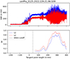 |
Figure 1 Example of Spire high rate 50 Hz GNSS-RO conPhs extended profile. Top panel: SNR, bottom panel: corresponding S4 values. The profile is acquired on 2022-08-17 (DOY 229) at 21:06 UTC with S125 as the receiver Rx and GPS PRN09 as the transmitter Tx. |
In normal operation, the STRATOS receiver only collects 50 Hz GNSS-RO data up to a straight-line tangent altitude (SLTA) of 170 km (Spire, 2021). However, for the GPS constellation only, the receiver has been modified to include an onboard scintillation detector. If an ionospheric scintillation event is triggered, then the 50 Hz measurements are recorded and downlinked over an extended altitude range, i.e., from the LEO orbit altitude (400–650 km) to below Earth’s surface (Spire, 2021). We refer to such measurements as “extended profiles”.
4 Additional datasets
4.1 COSMIC-2 Electron Density profiles (COSMIC-2 ionPrf)
The COSMIC-2/FORMOSAT-7, henceforth referred to as COSMIC-2, is a joint Taiwan-US mission. It is a constellation of six LEO satellites at an inclination of 24° with the objective of producing a uniform and continuous collection of atmospheric and ionospheric data for several applications like near-real-time terrestrial weather forecasts and space weather monitoring and climate studies (Straus, 2020). It hosts three payloads: a TGRS, an Ion Velocity Meter (IVM), and a radio frequency beacon.
The high-rate 50 Hz/100 Hz COSMIC-2 GNSS-RO Level1b product includes atmospheric excess phase (conPhs) files, which are commonly used for lower atmosphere sounding. The standard measurement tracks signals up to TP heights of about 130 km and therefore cannot be used for F-layer ionospheric retrievals. Hence, in this study, we have used the Level2 TGRS space weather product (ionPrf), which provides reprocessed Ne and TEC profiles. The data is available via the CDAAC repository (https://doi.org/10.5065/t353-c093). The TEC is measured along the RO path between the GNSS transmitter and the COSMIC-2 GNSS receiver. An Abel Transform inversion, assuming local ionosphere spherical symmetry, is applied to estimate the Ne profile (Hernández-Pajares et al., 2000; Hajj et al., 2002). Assuming that the plasma is frozen over the time of the RO event, small-scale fluctuations in TEC or Ne profiles are caused by plasma fluctuations in both the vertical and horizontal dimensions (Hocke et al., 2019). We have adopted the same detection technique to extract plasma fluctuations as described by Hocke et al. (2019). This uses a high-pass filter in the s domain, where s is defined as the distance between the highest and lowest TP heights. A digital non-recursive finite impulse response (FIR) high-pass filter with cutoff scale lengths of 50 km, with a Hamming window and the number of filter coefficients corresponding to three 50 km intervals, is used to identify fluctuations in both Ne and TEC profiles (Hocke et al., 2019).
An example of a disturbed ionPrf profile between one of the COSMIC-2 satellites (C2E1) and GLONASS PRN19 is shown in Figure 2. The acquisition is made over western Africa south of the geomagnetic equator under a geomagnetically active ionosphere. The blue curves in Figure 2a left and right panels are the original disturbed Ne and the high-pass filtered (Nehp,filt, with scale lengths <50 km) profiles, respectively. The low-pass filtered profile Nelp,filt has Ne fluctuations with a scale size greater than 50 km. It is obtained by subtracting the high-pass filtered output from the original Ne and is shown as the red curve overlaid on the original Ne in the left panel. The corresponding TEC profiles are shown in Figure 2b.
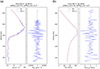 |
Figure 2 Example of perturbed Ne (a) and TEC (b) profiles from COSMIC-2 ionPrf data on 2022-08-17 at 19:38 UTC for a GLONASS-COSMIC-2 link. The latitude, longitude, and time of acquisition of the peak electron density (edMax) are given in the plot headers. The left panels of subplots show the original perturbed profiles in blue (Ne or TEC), and overlaid on them are the low-pass filtered profiles in red (Nelp,filt or TEClp,filt). The right panels show the high-pass filtered profile with fluctuations <50 km scale length (Nehp,filt or TEChp,filt). |
4.2 GOLD disk images (GOLD)
The GOLD mission (Eastes et al., 2017, 2019) was launched in 2018 with the main objectives of studying the response of Earth’s thermosphere-ionosphere to geomagnetic activity and investigating the formation and evolution of plasma irregularities in the ionosphere. GOLD obtains images of the Earth within the far ultraviolet band (~132–162 nm) from a geostationary satellite located at 47.5°W. Its field-of-view camera covers mainly the South American and Atlantic sectors and partly western Africa. The GOLD instrument has independent imagers for the Northern and Southern hemispheres, each observing the limb and the disk. The disk images contain calibrated and geolocated radiance data (GOLD Release Notes, 2022) (where radiance is expressed in Rayleigh, and 1 Rayleigh is a radiance unit equal to 106 photons emitted into 4π steradians from an area of 1 cm2) during the daytime, and the density of the ionospheric plasma at night (Eastes et al., 2017).
For this study, we have used the Level1C product of nighttime disk images at 135.6 nm using the low-resolution slit (NI1). The 135.6 nm wavelength band is used for monitoring atomic oxygen emission, which at night is generated by radiative recombination of O+ and can be used to derive information about the nighttime ionosphere (Eastes et al., 2017). The disk images are obtained independently on the two channels: Channel A (CHA) and Channel B (CHB), which scan the two hemispheres, approximately every 15 min. A reference altitude of 300 km is considered for geolocating the NI1 data pixels (GOLD Release Notes, 2022).
Figure 3 shows an example of the combined CHA and CHB GOLD Level1C NI1 data over West Africa. The Northern and Southern crests of the EIA are demarcated by the increased radiance on both sides of the geomagnetic equator (black dotted line). The patches of decreased emissions, between the crests, indicate depletions in plasma caused by instabilities in the ionosphere (Eastes et al., 2019; Karan et al., 2020; Aa et al., 2023). These are equatorial plasma bubbles, and they expand away from the geomagnetic equator to higher magnetic latitudes as they grow during the evening. These EPBs are one of the many drivers of F-layer scintillation in post-sunset low latitudes (Basu et al., 1988, 2002). In Figure 3, we can see three distinct EPBs (B1, B2, and B3) enclosed within a yellow oval. Slowly drifting eastward during the evening, these EPBs have a longitudinal extent between 4° and 8°, which is approximately 450–900 km at the equator.
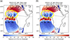 |
Figure 3 Examples of GOLD Level1C Nighttime (NI1) disk scans at 135.6 nm on 2022-08-17 at (a) 20:55 UTC and after 15 min at (b) 21:10 UTC. Scans from both channels A and B are combined to present the complete image. The Northern and Southern crests of the EIA can be observed with increased radiance on either side of the geomagnetic equator, marked by the black dotted line. Three EPBs, B1, B2, and B3, are highlighted by black arrows enclosed within a yellow oval. |
We also used the daytime disk images (L1C DAY) at 135.6 nm and the wavelengths for molecular Nitrogen (the Lyman-Birge-Hopfield, LBH bands) for the quiet period analyses. During the daytime, the CHA of the GOLD imager takes disk images of the Earth in high resolution (HR) mode at a cadence of 2 hours. For each hemisphere, the channel scans the dayside disk in two swaths, each taking 12 min, i.e., if CHA starts scanning the Northern hemisphere at 08:10 UTC, then after 12 min, at 08:22 UTC, the Southern hemisphere scan starts. The total scan takes 24 min to complete. Unlike the pronounced atomic oxygen emission at 135.6 nm during the night, the molecular nitrogen emissions at the LBH wavelengths dominate during the day. Laskar et al. (2021a, b) have used the LBH data to retrieve neutral disk temperatures. The top row of Figure 4 shows the combined daytime disk scans at 135.6 nm (left panel, Figure 4a) and the LBH band (right panel, Figure 4b) emissions between 12:10 and 12:34 UTC. It should be noted that for day disk scans, the reference altitude for measurements is 150 km, unlike 300 km for night scans (GOLD Release Notes, 2022). The absolute radiance values at daytime are much higher compared to nighttime, and hence the data is plotted in units of kilo Rayleigh (kR). We can observe the formation of the EIA gradually in both bands between 12:10 and 12:34 UTC. The two crests and the trough are clearer in the LBH bands since they dominate during the day. As the day progresses, the EIA crest in the north becomes more prominent (bottom row, Figs. 4c–4d, taken between 16:10 and 16:34 UTC) in the LBH band, compared to the southern EIA crest. This inter-hemispheric asymmetry has been previously reported (Vila, 1971; Loutfi et al., 2022). The EIA features slowly disappear from the daytime scans and start appearing in the nighttime images, as shown in Figure 3. Daytime scans for the remaining timestamps are provided in Figure S1 of Supplementary file S1.
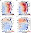 |
Figure 4 Examples of GOLD Level1C daytime (DAY) disk scans on 2022-08-17 from 135.6 nm wavelength in the left panels and LBH bands in the right panels, top: (a)–(b) between 12:10 and 12:34 UTC, and bottom: (c)–(d) between 16:10 and 16:34 UTC. CHA scans from both hemispheres are combined to present the complete image. |
4.3 ICON ion density (ICON)
The ICON mission, launched in 2019 and at an average altitude of 575 km with a 27° inclination angle in a circular orbit, is designed to measure plasma parameters (Immel et al., 2018). The IVM onboard ICON records ion density, drift velocities, composition, and temperature at a data rate of 1 Hz (Heelis et al., 2017; Immel et al., 2018). The ion density measurements can be used to detect topside ionospheric irregularities as reported by (Park et al., 2021; Choi et al., 2023).
To identify fluctuations in the ion density (Ni) due to ionospheric irregularities, we follow the same procedure as described in Park et al. (2021). First, the Ni data is detrended to remove the background trends ( ) using a Savitzky-Golay filter (Osei-Poku et al., 2021; Pakhotin et al., 2021) of 2nd order and a window size of 31 s. The fluctuations are identified by setting a threshold value for the absolute value of the residual ion density, i.e.,
  . Following Stolle et al. (2006), this threshold for
  is set at 3 × 10⁹ m−3. If |∆Ni| exceeds the threshold for 10 s consecutively, then an “irregularity event” is recorded. The measurements of the in situ Ni and |∆Ni | computed using the above-described method along the satellite trajectory are shown in Figure 5. Similar to Park et al. (2021), we have highlighted irregularity events lasting for 20 s in yellow to have sufficiently large data points for comparison. A detailed description of other IVM parameter measurements is provided in Park et al. (2021, 2022).
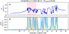 |
Figure 5 ICON ion parameters of (a) ion density Ni, and (b) computed absolute value of residual ion density |∆Ni|, identifying irregularity events for Track 15575 on 2022-08-17. Time at the midpoint of shown track segment is 20:50 UTC. The black dotted line in panel (b) is the threshold of |∆Ni| used for irregular event detection. The yellow shaded sections refer to the irregularity events detected and lasting for 20 s along this satellite track, and the segment later used for investigation is shaded in reddish color. |
5 Results and discussion
5.1 Disturbed period analysis
5.1.1 Event 1: 2022-08-17, DOY 229, 1800–2400 UTC
Maps of TPs from Spire RO measurements over Africa for a perturbed and a quiet period are shown in Figure 6. The TPs are color-coded with the S4 calculated from the L1 50 Hz SNR measurements. It is evident from the S4 maps that during the selected ionospherically perturbed period (Fig. 6a), a large number of profiles show high (i.e., >0.5) S4 values. On the contrary, during the selected ionospherically quiet time, for most cases, the S4 is less than 0.2 (Fig. 6b). Additionally, the Spire TP tracks are shorter (i.e., <170 km TP heights) during the quiet period since no scintillation is detected, and consequently, the extended profiles are not downlinked and stored in the data archive.
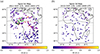 |
Figure 6 S4 map at L1 from all GNSS RO profiles from Spire’s CubeSat constellation over the African region on 2022-08-17 during (a) ionospherically perturbed period, 1800–2400 UTC, and (b) ionospherically quiet period, 1200–1800 UTC. The two RO profiles enclosed within green circles in panel (a) are used for further analysis. |
For this perturbed period, we specifically focus on two extended GNSS-RO profiles highlighted by the green circles (Fig. 6a). We denote the profile encircled in green to the south of the geomagnetic equator, marked by the black dotted line in the figure, as Spr1 and the profile to the north of it as Spr2. The SNR and S4 plots of these two profiles are shown in Figure 7. The two GNSS-RO profiles are acquired at the same time and from the same Tx (GPS PRN23). While Spr1 (Fig. 7a) has an average S4 of 0.71 between 150 and 400 km TP height, the average S4 for Spr2 (Fig. 7b) between the same heights is 0.33. Nevertheless, the signal fluctuations in both extended profiles indicate the presence of ionospheric irregularities causing amplitude scintillation in GNSS-RO signals at F-layer heights. This is consistent with the literature on the origin and morphology of scintillation in the post-sunset equatorial regions (Koster, 1972; Aarons, 1977, 1982, 1993; Basu et al., 1977). However, it is a challenge to precisely geolocate these irregularities along the long RO propagation path. Carrano et al. (2017) have demonstrated the geolocation of irregularities causing scintillation in GNSS-RO signals and validated their results with C/NOFS and GOLD data. However, as a first-order approximation, it can also be assumed that the irregularities are located at the TP provided that the F-layer peak is not significantly higher than the TP (Straus et al., 2003; Whalen, 2009; Dymond, 2012). In this study, we have used this approximation.
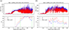 |
Figure 7 SNR and S4 plots of two 50 Hz Spire’s GNSS RO profiles highlighted in Figure 6a that are discussed as examples of a disturbed event on 2022-08-17 at 20:56 UTC. These profiles, Spr1 and Spr2, have the same Tx: GPS PRN23, but different Rxs: S135 and S127, respectively. The segment of the profile enclosed between the green dashed lines is later used for comparison with the COSMIC-2 data shown in Figure 8. |
The presence of ionospheric irregularities causing scintillation in the Spire data is investigated using colocated COSMIC-2 ionPrf, GOLD, and ICON data. We defined the following colocation criteria for Spire, COSMIC-2, and ICON data when comparing with an EPB detected in the GOLD NI1 image at a particular timestamp. They are as follows:
The geographic longitude of at least one measurement point, mapped to 300 km GOLD reference height, must lie within ±5° of the center of an EPB.
At least one measurement point must lie within a ± 15-minute time window from the time of GOLD acquisition.
To compute the center of EPBs from a GOLD nighttime disk scan, we implement the technique elaborated in Karan et al. (2020) and Aa et al. (2023). For the sake of brevity, we do not explain the detailed steps. Furthermore, the typical zonal scale size of EPBs can vary between a few to 10 degrees (Aa et al., 2020, 2023; Huba & Liu, 2020). Hence, the size of the longitudinal search window is set to ±5° from the center of an EPB.
Since all the satellite measurements are at different altitudes, we use the CHAOS (CHAMP, Ørsted, SAC-C, Cryosat-2, and SWARM) magnetic field model (Finlay et al., 2020) to map individual measurement points along the magnetic field lines (i.e., geocentric distances of 6,371.2 km plus LEO trajectory or TP heights) to the reference GOLD altitude of 300 km (see Park et al., 2022 for details). This ensures that the positions of different satellite measurements are mapped to the same reference altitude for appropriate comparison.
For example, the central geographic longitudes of EPB B1, B2, and B3 in the GOLD nighttime scan at 20:55 UTC (shown in Fig. 3) are approximately 11.7°W, 6.8°W, and 4.6°E. The longitudes of the nearly 12000 TP measurement points in the 50 Hz Spr2 profile (only TP heights > 40 km) span between 5° and 10°E and are within 20:53–20:59 UTC. This fulfills our first criterion of colocated measurement, i.e., the geographic longitude of at least one measurement point, mapped to 300 km GOLD reference height, must lie within ± 5° of the center of an EPB. Next, we choose two COSMIC-2 profiles (denoted as Csm1 and Csm2 in Fig. 8) based on the second criterion. The 1 Hz Csm1, with a total of 332 measurement points, spans from 18°W to 18°E, crossing all three EPB centers between 20:58 and 21:04 UTC. However, the acquisition time does not coincide with the GOLD data. To account for instances, such as Csm1, we implement the additional criterion of a ±15-minute time search window. In addition, Csm1 and Csm2 were collected within 4 min of the Spire profiles.
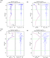 |
Figure 8 Same as Figure 2, except for the acquisition shown in (a) and (b) are for the COSMIC-2 ionPrf Csm1 with Tx: GLONASS PRN17 and Rx: C2E6 on 2022-08-17 at 20:57 UTC, and (c) and (d) are for Csm2 with Tx: GLONASS PRN24 and Rx: C2E6 on 2022-08-17 at 20:59 UTC. |
For each of the COSMIC-2 ionPrfs, we performed the high-pass filtering on both Ne and TEC described in Section 4.1 to identify fluctuations due to irregularities (Fig. 8). To compare the two datasets (Spire and COSMIC-2) at similar TP heights, we selected only a segment of the Spire conPhs profiles and COSMIC-2 ionPrfs between TP heights of 150–400 km, highlighted by the green dotted lines in Figures 7 and 8, respectively. For both the COSMIC-2 profiles, the Nehp,filt and TEChp,filt plots show large fluctuations between 300 and 500 km TP heights. In Csm1, the TEC fluctuations close to 500 km are as high as 10 TECU. Csm2 also shows a high TEChp,filt on the order of a few TECUs. One reason for the variability in Ne and TEC below 80 km TP height in profile Csm2 can be due to horizontal fluctuations that are not differentiated from small-scale fluctuations in the vertical direction (Hocke et al., 2019). Another explanation can be that the small-scale irregularities are distributed along the complete ray path between the transmitter GNSS and receiver LEO satellites (Carrano et al., 2017).
By applying the technique of plasma irregularity detection described in Section 4.3, we identified multiple irregularity events in the ICON track 15575 shown earlier in Figure 5. These events are highlighted by the yellow-shaded segments in the figure. Some of the irregular events span greater than 3° in longitude. This may indicate several small-scale fluctuations inside a larger irregular structure. This is similar to plasma blobs previously reported by Park et al. (2022). The part of the ICON track used in this analysis is shaded in reddish color (Fig. 5).
Figure 9 shows the position of all the measurements used in the analysis of this event. S4 is a measure of variability in the signal intensity, a second-order moment. In order to have a fair comparison with S4, we computed the second-order moments for the corresponding COSMIC-2 and ICON measurements, i.e., variance of TEChp,filt and variance of |∆Ni|, respectively. The top panel (a) of Figure 9 shows the map of S4, the variance of TEChp,filt, and variance of |∆Ni| computed from colocated Spire, COSMIC-2, and ICON measurements, respectively, with different color scales. The GOLD NI1 radiance image at 20:55 UTC is plotted in the background. The longitudinal variations of each measurement type are shown in Figure 9b. For example, we use the S4 index for Spire profiles, TEChp,filt (left panel) and variance of TEChp,filt (right panel) for COSMIC-2 data, and |∆Ni| (left panel) and variance of |∆Ni| (right panel) for ICON measurements.
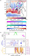 |
Figure 9 (a) Map with different sensor measurements color-coded and overlaid on the GOLD nighttime radiance image for perturbed Event 1 on 2022-08-17 between 20:50 and 21:10 UTC. The two Spire RO profiles are denoted as Spr1 and Spr2, and the COSMIC-2 profiles as Csm1 and Csm2. (b) Longitudinal variation of individual measurements mapped to 300 km reference altitude, as the GOLD data using the CHAOS model are plotted along the geographic longitude. |
For the Spire GNSS-RO data, the position of TPs in profile Spr1, where S4 values are marked in green (Fig. 9b) lies between the southern crest of EIA and EPB B3, encircled in black. The presence of high S4 values (Fig. 7a) due to small- (Fresnel) scale irregularities at the edges of plasma bubbles is consistent with the study reported by Spogli et al. (2023). On the other hand, profile Spr2 marked in magenta (Fig. 9b), is inside EPB B3 and exhibits lower S4 (Fig. 7b). The TEChp,filt and its variances at TPs of Csm1 (dotted lines) and Csm2 (solid lines) are shown in Figure 9b middle panel, in blue and brown respectively. We observe high fluctuations in both TEChp,filt and its variance in both profiles, which indicates irregular structures with scale lengths smaller than 50 km. Likewise, ICON measurements of |∆Ni| and its variance (see orange and purple plots, respectively) in the bottom panel of Figure 9b indicate irregularity events detected during the evening of 2022-08-17. All measurements shown in Figure 9 are mapped along the magnetic field lines at the GOLD reference altitude of 300 km. As a result, there is a small shift observed in the positions of COSMIC-2, Spire, and ICON. For example, in the segment of the ICON track shaded in reddish color (Fig. 5), the starting point is now shifted from (4.5°N, 1.9°W) to about (3.4°N, 3.18°W). The close spatial and temporal proximity of different satellite measurements with simultaneous detection of fluctuations in the TEC and ion density variance confirm that the large S4 values found in the Spire RO data are caused by ionospheric irregularities.
5.1.2 Event 2: 2022-03-28, DOY 087, 1800–2400 UTC
Another ionospherically perturbed event has been analyzed on 2022-03-28, DOY 087 between 20:50–21:10 UTC. The SNR and S4 measurements of a Spire extended profile, Spr3, are shown in Figure 10. In this example, we observe one clear scintillating signal segment starting from around 150 km TP height until the end of the extended profile at ~450 km with an average S4 at L1 of 0.87. The Spire GNSS-RO profile was acquired during post-sunset local time LT (corresponding to 18–24 UTC), and we can investigate whether the signal fluctuations can be attributed to ionospheric irregularities due to EPB by comparison with the other sensor measurements. We consider the segment of the extended profile between 150 and 450 km, marked between the two green dashed lines, for further analysis.
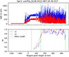 |
Figure 10 SNR and S4 plot of one of the extended GNSS-RO profiles Spr3 for the evening of 2022-03-28 at 20:45 UTC that is discussed in this section. The profile has Tx: GPS PRN17 and Rx: S128. |
In the absence of extended high-rate GNSS-RO measurements from COSMIC-2, we rely on the automatic irregularity detection algorithm described in Section 4.1 to identify small-scale plasma structures that may cause scintillation. In Figures 11a–11b, we show the high-pass filtered fluctuations in Ne and TEC, respectively, of a COSMIC-2 profile Csm3, which is in close temporal and spatial proximity (see colocation criteria in Sect. 5.1.1) with other sensor measurements. To compare TP positions at the same altitude in COSMIC-2, we choose the same altitude range, 150–450 km, as the Spire Spr3 profile. Between TP heights of 220–400 km, the TEChp,filt is >3 TECU, attributed to irregularities with smaller scale lengths in the F-region. During the same evening, there was also an ICON track that detected irregular events along the satellite trajectory marked as fluctuations in |∆Ni|. The Ni and |∆Ni| measurements from the ICON track 13452 on 2022-03-28, centered at 20:52 UTC, are shown in Figure 11c. The |∆Ni| measurements in the second panel show multiple irregularity events detected (marked in yellow shade) using the algorithm described in Section 4.3. The reddish-shaded segment in the track is used for comparative analysis.
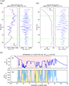 |
Figure 11 (a), (b) Same as Figure 2, except for the acquisition shown for COSMIC-2 profile Csm3, Tx: GLONASS PRN14 and Rx: C2E6, on 2022-03-28. (c) Same as Figure 5 for track 13452 on 2022-03-28 and the time at the midpoint of shown track segment is 20:52 UTC. |
The presence of irregularities in the post-sunset ionosphere is confirmed by the presence of EPBs in the nighttime GOLD images shown in the background of Figure 12. We used the GOLD nighttime disk image captured at 20:55 UTC, around the same time when the Spire, COSMIC-2, and ICON measurements were acquired. We can clearly observe the structure of EPBs in the form of stripes across the geomagnetic equator between the Northern and Southern crests of EIA. Strong variations in the ICON’s |∆Ni| and variance of |∆Ni| values can be seen as the spacecraft trajectory crosses multiple EPBs. The S4 from Spire and the variance of TEChp,filt (as well as TEChp,filt) from COSMIC-2 are larger. The evidence of EPBs in GOLD data and small-scale irregularities in COSMIC-2 ionPrf indicates that the strong amplitude scintillation observed in Spire data is caused by ionospheric irregularity structures. Similar to Figure 9, in Figure 12, we have also mapped the TP positions of Spire and COSMIC-2 ionPrf and the ICON track along the magnetic field lines to the GOLD’s reference altitude of 300 km using the CHAOS model. Due to this, the locations of satellite measurements are slightly shifted, for example, the ICON track is shifted from (4.9°N, 15°S) to (3.3°N, 17°S). Similar shifts are also observed for the GNSS-RO data from Spire and COSMIC-2. The daytime disk scans from GOLD for the date are shown in Figure S2 of Supplementary file S1.
5.2 Quiet period analysis
In the previous subsection, we discussed two perturbed events where we have evidence of ionospheric irregularities from multiple sensors that may have caused the scintillation observed in Spire RO data. In this subsection, we compare measurements from the same sensors during quiet ionospheric conditions during 1200–1800 UTC over the African region. For brevity, we discuss only one quiet event on 2022-08-17 around 12:15 UTC. No extended GNSS-RO Spire conPhs profiles were found during this period. This is because, during local daytime, no F-region amplitude scintillation events trigger the onboard detector, resulting in no extended profiles being downlinked. We have therefore used GOLD daytime disk images, ICON measurements, and COSMIC-2 ionPrfs to confirm the absence of ionospheric irregularities.
During the daytime, we do not observe any EPBs in the GOLD daytime disk images. Hence, our criteria for acquiring colocated measurements from COSMIC-2 and ICON are modified from the previously described nighttime criteria in Section 5.1.1. The ICON track is selected considering the time window of GOLD measurement (12:10–12:34 UTC) and spatial boundaries covering the African sector (± 45° geographic latitudes and 20°W–50°E geographic longitudes). The GOLD data analyzed during the quiet period are already shown in Figure 4. Radiances at both 135.6 nm and the LBH bands do not show any signs of EPBs. The ICON measurements of ion density Ni and irregularity estimate |∆Ni| for the quiet time event on 2022-08-17 are shown in Figure 13. Between 1200 and 1800 UTC, there were four ICON tracks over Africa, but only track number 15570 is shown since it is acquired within the time window of GOLD data. This track lies to the south of the EIA between 22 and 27°S latitudes. The Ni plot is relatively smooth (Fig. 13a) and |∆Ni| values are below the irregularity detection threshold (black dotted line in Fig. 13b). These results indicate quiet ionospheric conditions during daytime over the area under study.
Two COSMIC-2 ionPrfs, shown in Figure 14, are also acquired such that at least one measurement point is within ±1° geographic latitude/longitude from the ICON track during the GOLD acquisition time window. The ionPrfs are very smooth and do not exhibit any significant fluctuations in either Ne or TEC for TP heights greater than 130 km. Thus, no F-layer irregularities were detected during this time. Fluctuations are observed around 100 km altitude, which may correspond to strong vertical gradients in the sporadic E-layer. This analysis is, however, outside the scope of the current paper.
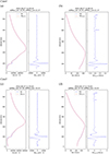 |
Figure 14 Same as Figure 2, except for the acquisition shown in top panel: (a) and (b) are for COSMIC-2 ionPrf Csm4 at 12:29 UTC, and bottom panel: (c) and (d) for Csm5 at 12:34 UTC. For both the profiles shown, the RO link is between Rx COSMIC-2 satellite C2E6 and Txs GPS PRNs (G26 and G20) on 2022-08-17. |
Although we have shown only one example of an ionospherically quiet period in this work, the result remains similar for other days too, i.e., no extended Spire profiles were detected during local daytime 1200–1800 UTC over the African longitude sector. Furthermore, neither evidence of EPB occurrence in GOLD images nor signatures of F-layer irregularities in the COSMIC-2 ionPrf or the in-situ ICON ion density measurements are observed. A combined plot similar to Figure 9 for the described quiet period example is provided in Figure S3 of Supplementary file S1.
5.3 Long-term analysis
In this section, we compare the occurrence statistics of F-region scintillation or irregularity events in the low-latitude African and American sectors using Spire’s 50 Hz conPhs GNSS-RO and COSMIC-2 1 Hz ionPrfs data. The African and American longitude sectors are defined between 20°W–50°E, and 90°W–30°W, respectively. Keeping in mind that the latitudinal coverage of COSMIC-2 is limited compared to Spire, we restrict this comparison to ±40° geographic latitudes. While we have a full database for COSMIC-2 datasets starting from October 1st, 2019, the Spire files are restricted to those available on the COSMIC/UCAR public repository. Nonetheless, we used all available datasets from October 2019 until December 2023 in this analysis. Furthermore, since F-layer scintillation is mostly observed in post-sunset equatorial regions, we have also constrained the analysis to data between 1800 and 0300 LT at the measurement TP.
A 50 Hz Spire conPhs profile is identified to have encountered a scintillation event if the S4 index at L1 exceeds 0.3 for TPs greater than 170 km. COSMIC-2 profiles are identified as perturbed when small-scale irregularities are detected by setting thresholds for Nehp,filt and TEChp,filt. The estimation of the perturbation profiles has been previously described in Section 4.1. The threshold criteria are as follows:
Tangent point height >170 km, and
Nhp,filt < −0.5e5 cm −3 or Nehp,filt > 0.5e5 cm−3, and
TEChp,filt < −1 TECU or TEChp,filt > 1 TECU.
If a COSMIC-2 ionPrf profile fulfilled the above three criteria, then it was marked as one that detected irregularities that might cause F-layer scintillation. For this long-term analysis, we chose the COSMIC-2 threshold criteria based on Nehp,filt and TEChp,filt, and not the second-order moments, variance of Nehp,filt or TEChp,filt. Our analysis from Figures 9 to 12 indicates that small-scale ionospheric irregularities with a scale length <50 km using COSMIC-2 can be detected well using both the high-pass filtered measurements (first-order moments) and their respective variances (second-order moments).
The solar activity in terms of the F10.7 index during the study period (Oct 2019 – Dec 2023) is presented in Figure 15a. Each year is divided into four seasons, and these are highlighted in the figure: Spring – March and April; (Northern hemisphere) Summer – May, June, July, and August; Autumn – September and October; (Northern hemisphere) Winter – November, December, January, February. We observe a gradual rise in F10.7, indicating the increase in solar activity for solar cycle 25, expected to peak in 2025 (Bhowmik & Nandy, 2018; Penza et al., 2023).
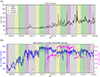 |
Figure 15 (a) Solar activity level index F10.7 for the period under study, (b) Total number of COSMIC-2 ionPrfs and Spire conPhs files available per day via UCAR repository. |
In Figure 15b, the total number of COMSIC-2 ionPrfs and Spire conPhs profiles available per day from the UCAR repository is plotted beginning from when COSMIC-2 data are first available (i.e., October 2019) until December 2023. From these daily downlinked data, profiles only in the low-latitude equatorial region between ±40° geographic latitudes are used for computation and statistical analysis of ionospheric irregularities or scintillation occurrence rate. In this study, we have excluded data for the days when Kp ≥ 6 for at least one 3-hourly window, thus excluding geomagnetically active days, which might affect the results for the climatology of post-sunset ionospheric irregularities observed in low-latitude equatorial regions.
Although the Spire CubeSats track GPS, GLONASS, and GALILEO constellations, the onboard amplitude scintillation detector is designed only for the GPS constellation. However, COSMIC-2 tracks both GPS and GLONASS constellations and detects irregularities for both cases. Therefore, to provide a fair comparison between the two constellations in detecting scintillation or irregularities, we have considered GPS data only. Figure 16 shows the daily occurrence rate (in percentage, i.e.,  ) of scintillation or irregularities detected in Spire and COSMIC-2 profiles during the selected time period over the African longitudinal (Fig. 16a), and American longitudinal (Fig. 16b) sectors. The daily occurrence rates are denoted by dots in the figures, and the 27-day running mean is denoted by the thick colored lines (blue for COSMIC-2 and magenta for Spire). We chose a 27-day running mean considering the Sun rotation cycle, which is a better representation of solar parameters, such as the F10.7, used in this study.
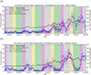 |
Figure 16 Statistics of scintillation or irregularities occurrence rates from COSMIC-2 and Spire data, for GPS constellation only over (a) African longitudinal, and (b) American longitudinal sectors. Data between ± 40° geographic latitudes and 1800 – 0300 LT have been used. |
The gaps visible in the Spire statistics are due to the unavailability of data in the repository. Nevertheless, we see similar and consistent trends in the irregularity occurrence rates obtained from both Spire and COSMIC-2 during mid-September 2021 to April 2023. This is encouraging since we are using two different satellite constellations and different detection techniques for the GNSS-RO data. From May to mid-July 2023 (when Spire data is last available), there were no extended profiles detected in the Spire data. The highest TP of RO profiles during this period was found to be about 150 km. Thus, no F-layer scintillation detection was possible. The 150 km cutoff is due to the pre-processing of the raw RO data during this interval, performed at UCAR before it is made publicly available (Nguyen, 2024). It is further confirmed that there was no technical issue with the onboard scintillation detector during this period, preventing the download of extended profiles (Nguyen, 2024).
Over the African longitude sector, the irregularity occurrence rates have pronounced maxima during the equinox (spring and autumn) months. A significant minimum is also observed during the northern solstice, with a secondary minimum during the winter months. The irregularity occurrence rates from COSMIC-2 and Spire are in good agreement with previous studies on the climatology of equatorial ionospheric irregularities or scintillation (Koster, 1972; Aarons, 1977, 1982). Carter et al. (2013) in their paper on occurrence statistics of equatorial F-layer irregularities (EFIs) using COSMIC GNSS-RO reported the highest (least) EFI occurrence over the American longitudinal sector during the December (June) solstice. Their paper is in good agreement with our findings from COSMIC-2 (Spire) irregularity (scintillation) detection that the occurrence rates over the American longitudes predominantly have large values in the period between September – March, with the highest rates around the December solstice and the lowest rates during summer months. Our results also agree well with previously reported climatological studies over the region (Muella et al., 2017; Macho et al., 2022). Similar seasonal dependencies of scintillation occurrence rates over the African longitudes have also been reported by Akala et al. (2015) in their investigation of this region using ground-based GNSS measurements.
Another interesting observation from the irregularity occurrence rate statistics is the increased rates from the Spire constellation over American longitudes during the equinox months (March–April and September–October) compared to COSMIC-2. The exact reason is not known; however, different orbit inclinations of Spire (low and high) and COSMIC-2 (low) satellites may contribute to this. Furthermore, the integrated 1 Hz TEC measurements from COSMIC-2 are smoother compared to the 50 Hz SNR measurements from Spire and therefore are not able to sample the full scintillation spectrum. It may be due to this lower sampling rate that we miss some detections in the COSMIC-2 TEC data compared to the 50 Hz Spire data, which can be more representative of the physical phenomenon. Due to the integrated nature of the TEC data, care needs to be taken while using such data so that we do not miss out on detecting ionospheric irregularities. In principle, TEC should be compared with S4 only when RO signals are affected by deterministic effects (like refraction), and there are no stochastic effects on the signal (Rino et al., 2019; McCaffrey & Jayachandran, 2022). Nevertheless, further investigation is needed, and this would be best done considering GNSS-RO data from a wider range of sources (i.e., the GeoOptics and PlanetiQ constellations). In general, for the American longitudinal sector, the Spire constellation has a slightly higher occurrence rate compared to the COSMIC-2. However, both constellations show similar and consistent variations of ionospheric irregularities or scintillation occurrence rates.
Furthermore, with COSMIC-2 ionPrfs being available for more than three years, a direct relation to solar activity is also evident (Fig. 16). The number of COSMIC-2 profiles detecting irregularities increases with solar activity, which is in agreement with previous irregularity or scintillation studies over the equatorial region (Aarons, 1977, 1982; Aarons et al., 1981; DasGupta et al., 1981; Correia et al., 2019).
6 Summary and conclusion
The presence of irregularities in the post-sunset equatorial ionosphere has been previously demonstrated in studies using both ground-based and space-based sensors. In this paper, we have presented evidence of ionospheric scintillation detection in the F-layer using high-rate GNSS radio occultation data from Spire’s CubeSat constellation. Extending on prior research in this area, Spire 50 Hz GNSS receiver measurements of SNR have been utilized to compute the amplitude scintillation index S4. We observed clear diurnal variations in the occurrence of F-layer scintillation. Furthermore, the Spire data did not exhibit scintillation at F-layer altitudes during daytime hours (1200–1800 UTC, LT = UTC to UTC + 1). This is consistent with the expected climatology of the African longitudinal sector, where equatorial plasma bubbles frequently occur during post-sunset local time (approximately 1800–2400 UTC).
Three events have been analyzed: two during periods of ionospheric perturbations and one at an ionospherically quiet time. During post-sunset hours of perturbed conditions, we found signatures of strong scintillation in the Spire GNSS-RO signals. The presence of ionospheric irregularities that cause scintillation has been verified using independent measurements from the COSMIC-2, GOLD, and ICON satellite missions. Irregularities are detected using Ne and TEC profiles from COSMIC-2, plasma densities based on oxygen emission lines measured by GOLD, and in situ ion density measurements from ICON. Results from the quiet period analyses are also consistent between the different sensors – in this case, no irregularities and no scintillation were detected.
Scintillation statistics from the Spire and COSMIC-2 GNSS-RO constellations have been compared over a period of three years for local evening time in two equatorial regions (African and American sectors). As expected, there is a direct relation between the scintillation occurrence rate and the increase in the solar activity level (F10.7) over the test period. Furthermore, data from both constellations were consistent with the expected climatology: for the African longitudes, irregularities/scintillation occurrence was higher during the equinoxes, whilst for the American sector, the occurrence rates are larger during September–April, with the highest during the December solstice.
The results presented in this paper demonstrate the suitability of commercial CubeSat constellations such as Spire for augmenting ionospheric scintillation studies using the data available from COSMIC-2 and other institutional GNSS-RO missions. This capability can provide an important contribution to scintillation monitoring and can provide valuable input to space weather nowcasts and forecasts.
Acknowledgments
The authors would like to acknowledge the help from Dr. Vu Nguyen and Dr. Giorgio Savastano from Spire Global for the useful discussions in understanding the extended altitude GNSS-RO datasets. SM would also like to thank Dr. Jaeheung Park from the Korea Space Weather Research Center for his help in implementing the mapping function using the CHAOS Model. The editor thanks Stephan Buchert and Anton Kashcheyev for their assistance in evaluating this paper.
Data availability statement
The GNSS-RO datasets from Spire and COSMIC-2 are open to the public at the UCAR website (https://data.cosmic.ucar.edu/gnss-ro/). The GOLD and ICON data are openly available on their respective websites https://gold.cs.ucf.edu/data/ and https://icon.ssl.berkeley.edu/Data.
Supplementary material
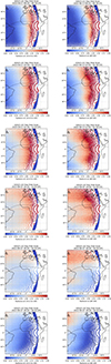 |
Figure S1: Daytime GOLD disk images from 135.6 nm wavelength (left panel) and LBH bands (right panel) on 2022-08-17. |
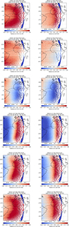 |
Figure S2: Daytime GOLD disk images from 135.6 nm wavelength (left panel) and LBH bands (right panel) on 2022-03-28 |
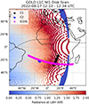 |
Figure S3: Map with different sensor measurements color-coded and overlaid on the GOLD’s daytime radiance image for quiet time event on 2022-08-17. C1 = Csm4 COSMIC-2 ionPrf, C2 = Csm5 COSMIC-2 ionPrf as described in Figure 14 of the main text, and ICON = ICON Track 15570 on 2022-08-17 as described in Figure 13 of the main text. |
S. Syndergaard (2006), COSMIC S4 data. Available at https://cdaac-www.cosmic.ucar.edu/cdaac/doc/documents/s4_description.pdf.
References
- Aa, E, Zhang S, Liu G, Eastes RW, Wang W, Karan DK, Qian L, Coster AJ, Erickson PJ, Derghazarian S. 2023. Statistical analysis of equatorial plasma bubbles climatology and multi‐day periodicity using GOLD observations, Geophys Res Lett 50 (8): e2023GL103510. https://doi.org/10.1029/2023GL103510. [CrossRef] [Google Scholar]
- Aa, E, Zou S, Eastes R, Karan DK, Zhang S, Erickson PJ, Coster AJ. 2020. Coordinated ground‐based and space‐based observations of equatorial plasma bubbles. J Geophys Res Space Phys 125 (1): e2019JA027569.https://doi.org/10.1029/2019JA027569. [CrossRef] [Google Scholar]
- Aarons, J. 1977. Equatorial scintillations: A review. IEEE Trans Antenna Propag 25 (5): 729–736. https://doi.org/10.1109/TAP.1977.1141649. [CrossRef] [Google Scholar]
- Aarons, J. 1982. Global morphology of ionospheric scintillations. Proc IEEE 70 (4): 360–378. https://doi.org/10.1109/PROC.1982.12314. [CrossRef] [Google Scholar]
- Aarons, J. 1993. The longitudinal morphology of equatorial F-layer irregularities relevant to their occurrence. Space Sci Rev 63 (3–4): 209–243. https://doi.org/10.1007/BF00750769. [CrossRef] [Google Scholar]
- Aarons, J, Whitney HE, MacKenzie E, Basu S. 1981. Microwave equatorial scintillation intensity during solar maximum. Radio Sci 16 (5): 939–945. https://doi.org/10.1029/RS016i005p00939. [CrossRef] [Google Scholar]
- Abdu, MA, MacDougall JW, Batista IS, Sobral JHA, Jayachandran PT. 2003. Equatorial evening prereversal electric field enhancement and sporadic E layer disruption: A manifestation of E and F region coupling. J Geophys Res Space Phys 108 (A6): 2002JA009285. https://doi.org/10.1029/2002JA009285. [CrossRef] [Google Scholar]
- Ahmed, IF, Alheyf M, Yamany MS. 2024. PlanetiQ radio occultation: Preliminary Comparative Analysis of Neutral Profiles vs. COSMIC and NWP Models. Appl Sci 14 (10): 4179. https://doi.org/10.3390/app14104179. [CrossRef] [Google Scholar]
- Akala, AO, Amaeshi LLN, Somoye EO, Idolor RO, Okoro E, et al. 2015. Climatology of GPS amplitude scintillations over equatorial Africa during the minimum and ascending phases of solar cycle 24. Astrophys Space Sci 357 (1): 17. https://doi.org/10.1007/s10509-015-2292-9. [CrossRef] [Google Scholar]
- Angling, MJ, Nogués-Correig O, Nguyen V, Vetra-Carvalho S, Bocquet F-X, Nordstrom K, Melville SE, Savastano G, Mohanty S, Masters D. 2021. Sensing the ionosphere with the Spire radio occultation constellation. J Space Weather Space Clim 11: 56. https://doi.org/10.1051/swsc/2021040. [CrossRef] [EDP Sciences] [Google Scholar]
- Basu, S, Aarons J, McClure JP, LaHoz C, Bushby A, Woodman RF. 1977. Preliminary comparisons of VHF radar maps of F-region irregularities with scintillations in the equatorial region. J Atmos Terr Phys 39 (9–10): 1251–1261. https://doi.org/10.1016/0021-9169(77)90034-4. [CrossRef] [Google Scholar]
- Basu, S, Groves KM, Basu Su, Sultan PJ. 2002. Specification and forecasting of scintillations in communication/navigation links: Current status and future plans. J Atmos Sol-Terr Phys 64 (16): 1745–1754. https://doi.org/10.1016/S1364-6826(02)00124-4. [CrossRef] [Google Scholar]
- Basu, S, MacKenzie E, Basu S. 1988. Ionospheric constraints on VHF/UHF communications links during solar maximum and minimum periods. Radio Sci 23 (3): 363–378. https://doi.org/10.1029/RS023i003p00363. [CrossRef] [Google Scholar]
- Beyerle, G, Schmidt T, Michalak G, Heise S, Wickert J, Reigber C. 2005. GPS radio occultation with GRACE: Atmospheric profiling utilizing the zero difference technique. Geophys Res Lett 32 (13): L13806. https://doi.org/10.1029/2005GL023109. [CrossRef] [Google Scholar]
- Bhowmik, P, Nandy D. 2018. Prediction of the strength and timing of sunspot cycle 25 reveal decadal-scale space environmental conditions. Nature Commun 9 (1): 5209. https://doi.org/10.1038/s41467-018-07690-0. [CrossRef] [Google Scholar]
- Brahmanandam, PS, Uma G, Liu JY, Chu YH, Latha Devi NSMP, Kakinami Y. 2012. Global S4 index variations observed using FORMOSAT-3/COSMIC GPS RO technique during a solar minimum year: GLOBAL S4 INDEX MAPS. J Geophys Res Space Phys 117 (A9). https://doi.org/10.1029/2012JA017966. [CrossRef] [Google Scholar]
- Carrano, CS, Groves KM, Rino CL, McNeil W. 2017, January. 2017 United States National Committee of URSI National Radio Science Meeting (USNC-URSI NRSM). Boulder, CO, USA, pp. 1–2. https://doi.org/10.1109/USNC-URSI-NRSM.2017.7878318. [Google Scholar]
- Carter, BA, Zhang K, Norman R, Kumar VV, Kumar S. 2013. On the occurrence of equatorial F‐region irregularities during solar minimum using radio occultation measurements. J Geophys Res Space Phys 118 (2): 892–904. https://doi.org/10.1002/jgra.50089. [CrossRef] [Google Scholar]
- CDAAC. 2023. UCAR: conPhs File Format. https://cdaac-www.cosmic.ucar.edu/cdaac/cgi_bin/fileFormats.cgi?type=conPhs. [Google Scholar]
- Chang, H, Lee J, Yoon H, Morton YJ, Saltman A. 2022. Performance assessment of radio occultation data from GeoOptics by comparing with COSMIC data. Earth Planet Space 74 (1): 108. https://doi.org/10.1186/s40623-022-01667-6. [CrossRef] [Google Scholar]
- Chang, H, Morton YJ, Dittmann T, Hunt D, Durgonics T, Braun J, Weiss J. 2025. Assessment of scintillation data from PlanetiQ and spire global radio occultation missions. J Geophys Res Space Phys 130 (3): e2024JA033543. https://doi.org/10.1029/2024JA033543. [CrossRef] [Google Scholar]
- Chen, S, Lin C(CH), Rajesh PK, Liu J, Eastes R, Chou M, Choi J. 2021. Near real‐time global plasma irregularity monitoring by FORMOSAT‐7/COSMIC‐2. J Geophys Res Space Phys 126 (1): e2020JA028339. https://doi.org/10.1029/2020JA028339. [CrossRef] [Google Scholar]
- Choi, J-M, Lin CC-H, Panthalingal Krishanunni R, Park J, Kwak Y-S, Chen S-P, Lin J-T, Chang M-T. 2023. Comparisons of in situ ionospheric density using ion velocity meters onboard FORMOSAT-7/COSMIC-2 and ICON missions. Earth, Planet Space 75 (1): 15. https://doi.org/10.1186/s40623-022-01759-3. [CrossRef] [Google Scholar]
- Correia, E, Tadeu de Assis Honorato Muella M, Alfonsi L, dos Santos Prol F, de Oliveira Camargo P. 2019. GPS Scintillations and Total Electron Content Climatology in the Southern American Sector. In: Accuracy of GNSS Methods , Ugur Sanli D (Ed.), IntechOpen Ltd, London, UK, pp. 47–70. https://doi.org/10.5772/intechopen.79218. [Google Scholar]
- DasGupta, A, Maitra A, Basu S. 1981. Occurrence of nighttime VHF scintillations near the equatorial anomaly crest in the Indian sector. Radio Sci. 16 (6): 1455–1458. https://doi.org/10.1029/RS016i006p01455. [CrossRef] [Google Scholar]
- Dymond, KF. 2012. Global observations of L band scintillation at solar minimum made by COSMIC. Radio Sci 47 (4): 2011RS004931. https://doi.org/10.1029/2011RS004931. [CrossRef] [Google Scholar]
- Eastes, RW, McClintock WE, Burns AG, Anderson DN, Andersson L, et al. 2017. The Global-Scale Observations of the Limb and Disk (GOLD) mission. Space Sci Rev 212 (1–2): 383–408. https://doi.org/10.1007/s11214-017-0392-2. [CrossRef] [Google Scholar]
- Eastes, RW, Solomon SC, Daniell RE, Anderson DN, Burns AG, England SL, Martinis CR, McClintock WE. 2019. Global‐scale observations of the equatorial ionization anomaly. Geophys Res Lett 46 (16): 9318–9326. https://doi.org/10.1029/2019GL084199. [CrossRef] [Google Scholar]
- Farley, DT, Balsey BB, Woodman RF, McClure JP. 1970. Equatorial spread F: Implications of VHF radar observations. J Geophys Res 75 (34): 7199–7216. https://doi.org/10.1029/JA075i034p07199. [CrossRef] [Google Scholar]
- Finlay, CC, Kloss C, Olsen N, Hammer MD, Tøffner-Clausen L, Grayver A, Kuvshinov A. 2020. The CHAOS-7 geomagnetic field model and observed changes in the South Atlantic Anomaly. Earth Planet Space 72 (1): 156. https://doi.org/10.1186/s40623-020-01252-9. [CrossRef] [Google Scholar]
- Forsythe, VV, Duly T, Hampton D, Nguyen V. 2020. Validation of ionospheric electron density measurements derived from spire CubeSat Constellation. Radio Sci 55 (1): e2019RS006953. https://doi.org/10.1029/2019RS006953, [CrossRef] [Google Scholar]
- GOLD Release Notes. 2022. GOLD Public Science Data Products Guide. https://gold.cs.ucf.edu/data/documentation/. [Google Scholar]
- Hajj, GA, Ao CO, Iijima BA, Kuang D, Kursinski ER, Mannucci AJ, Meehan TK, Romans LJ, e Juarez M, Yunck TP. 2004. CHAMP and SAC-C atmospheric occultation results and intercomparisons. J Geophys Res Atmos 109 (D6): D06109. https://doi.org/10.1029/2003JD003909. [CrossRef] [Google Scholar]
- Hajj, GA, Ibañez-Meier R, Kursinski ER, Romans LJ. 1994. Imaging the ionosphere with the global positioning system. Int J Imaging Syst Technol 5 (2): 174–187. https://doi.org/10.1002/ima.1850050214. [CrossRef] [Google Scholar]
- Hajj, GA, Kursinski ER, Romans LJ, Bertiger WI, Leroy SS. 2002. A technical description of atmospheric sounding by GPS occultation. J Atmos Sol-Terr Phys 64 (4): 451–469. https://doi.org/10.1016/S1364-6826(01)00114-6. [CrossRef] [Google Scholar]
- Hajj, GA, Romans LJ. 1998. Ionospheric electron density profiles obtained with the Global Positioning System: Results from the GPS/MET experiment. Radio Sci 33 (1): 175–190. https://doi.org/10.1029/97RS03183. [CrossRef] [Google Scholar]
- Heelis, RA, Stoneback RA, Perdue MD, Depew MD, Morgan WA, Mankey MW, Lippincott CR, Harmon LL, Holt BJ. 2017. Ion velocity measurements for the ionospheric connections explorer. Space Sci Rev 212 (1–2): 615–629. https://doi.org/10.1007/s11214-017-0383-3. [CrossRef] [Google Scholar]
- Hernández-Pajares, M, Juan JM, Sanz J. 2000. Improving the Abel inversion by adding ground GPS data to LEO radio occultations in ionospheric sounding. Geophys Res Lett 27 (16): 2473–2476. https://doi.org/10.1029/2000GL000032. [CrossRef] [Google Scholar]
- Hocke, K, Liu H, Pedatella N, Ma G. 2019. Global sounding of F region irregularities by COSMIC during a geomagnetic storm. Ann Geophys 37 (2): 235–242. https://doi.org/10.5194/angeo-37-235-2019. [CrossRef] [Google Scholar]
- Høeg, P, Hauchecorne A, Kirchengast G, Syndergaard S, Belloul B, Leitnger R, Rothleitner W. 1995. Derivation of atmospheric properties using a radio occultation technique. (DMI Scientific Report Nos. 95–4) DMI, pp. 1–205. [Google Scholar]
- Hoque, MM, Jakowski N. 2012. Ionospheric propagation effects on GNSS signals and new correction approaches. In: Global Navigation Satellite Systems: Signal, Theory and Applications, S, Jin (Ed.), InTech. https://doi.org/10.5772/30090. [Google Scholar]
- Huba, JD, Liu H‐L. 2020. Global Modeling of Equatorial Spread F with SAMI3/WACCM‐X. Geophys Res Lett 47 (14): e2020GL088258. https://doi.org/10.1029/2020GL088258. [CrossRef] [Google Scholar]
- Immel, TJ, England SL, Mende SB, Heelis RA, Englert CR, et al. 2018. The ionospheric connection explorer mission: Mission goals and design. Space Sci Rev 214 (1): 13. https://doi.org/10.1007/s11214-017-0449-2. [CrossRef] [Google Scholar]
- Jakowski, N, Wehrenpfennig A, Heise S, Reigber Ch, Lühr H, Grunwaldt L, Meehan TK. 2002. GPS radio occultation measurements of the ionosphere from CHAMP: Early results. Geophys Res Lett 29 (10): 95-1–95-4. https://doi.org/10.1029/2001GL014364. [CrossRef] [Google Scholar]
- Karan, DK, Daniell RE, England SL, Martinis CR, Eastes RW, Burns AG, McClintock WE. 2020. First Zonal Drift Velocity Measurement of Equatorial Plasma Bubbles (EPBs) From a Geostationary Orbit Using GOLD Data. J Geosphys Res Space Phys 125 (9). https://doi.org/10.1029/2020JA028173. [Google Scholar]
- Kepkar, A, Arras C, Wickert J, Schuh H, Alizadeh M, Tsai L-C. 2020. Occurrence climatology of equatorial plasma bubbles derived using FormoSat-3∕COSMIC GPS radio occultation data. Ann Geophys 38 (3): 611–623. https://doi.org/10.5194/angeo-38-611-2020. [CrossRef] [Google Scholar]
- Koster, JR. 1972. Equatorial scintillation. Planet Space Sci 20 (12): 1999–2014. https://doi.org/10.1016/0032-0633(72)90056-6. [CrossRef] [Google Scholar]
- Kursinski, ER, Hajj GA, Bertiger WI, Leroy SS, Meehan TK, et al. 1996. Initial results of radio occultation observations of Earth’s atmosphere using the Global Positioning System. Science 271 (5252): 1107–1110. https://doi.org/10.1126/science.271.5252.1107. [CrossRef] [Google Scholar]
- Larsen, GB, Syndergaard S, Høeg P, Sørensen MB. 2005. Single frequency processing of Ørsted GPS radio occultation measurements. GPS Solu 9 (2): 144–155. https://doi.org/10.1007/s10291-005-0142-x. [CrossRef] [Google Scholar]
- Laskar, FI, Eastes RW, Codrescu MV, Evans JS, Burns AG, Wang W, McClintock WE, Aryal S, Cai X. 2021a. Response of GOLD retrieved thermospheric temperatures to geomagnetic activities of varying magnitudes. Geophys Res Lett 48 (15): e2021GL093905. https://doi.org/10.1029/2021GL093905. [CrossRef] [Google Scholar]
- Laskar, FI, Pedatella NM, Codrescu MV, Eastes RW, Evans JS, Burns AG, McClintock W. 2021b. Impact of GOLD retrieved thermospheric temperatures on a whole atmosphere data assimilation model. J Geophys Res Space Phys 126 (1): e2020JA028646. https://doi.org/10.1029/2020JA028646. [CrossRef] [Google Scholar]
- Liu, L, Morton YJ. 2023. Assessment of storm-time ionospheric electron density measurements from Spire Global CubeSat GNSS radio occultation constellation. GPS Solu 27 (2): 75. https://doi.org/10.1007/s10291-023-01414-8. [CrossRef] [Google Scholar]
- Loutfi, A, Pitout F, Bounhir A, Benkhaldoun Z, Makela JJ, Abamni S, Zyane K, Elfakhiri A. 2022. Interhemispheric asymmetry of the Equatorial Ionization Anomaly (EIA) on the african sector over 3 years (2014–2016): effects of thermospheric meridional winds. J Geophys Res Space Phys 127 (9): e2021JA029902. https://doi.org/10.1029/2021JA029902. [CrossRef] [Google Scholar]
- Macho, EP, Correia E, Spogli L, Tadeu de Assis Honorato Muella M. 2022. Climatology of ionospheric amplitude scintillation on GNSS signals at south American sector during solar cycle 24. J Atmos Sol-Terr Phys 231: 105872. https://doi.org/10.1016/j.jastp.2022.105872. [CrossRef] [Google Scholar]
- Martinis, C, Daniell R, Eastes R, Norrell J, Smith J, Klenzing J, Solomon S, Burns A. 2021. Longitudinal variation of postsunset plasma depletions from the Global‐Scale Observations of the Limb and Disk (GOLD) mission. J Geophys Res Space Phys 126 (2): e2020JA028510. https://doi.org/10.1029/2020JA028510. [CrossRef] [Google Scholar]
- McCaffrey, A, Jayachandran PT. 2022. Comments on “Stochastic TEC structure characterization” by Charles Rino, Yu Morton, Brian Breitsch, and Charles Carrano. J Geophys Res Space Phys 124. https://doi.org/10.1029/2019JA026958; Journal of Geophysical Research: Space Physics, 127(1), e2021JA029423. https://doi.org/10.1029/2021JA029423. [Google Scholar]
- Muella, MTAH, Duarte-Silva MH, Moraes AO, de Paula ER, de Rezende LFC, Alfonsi L, Affonso BJ. 2017. Climatology and modeling of ionospheric scintillations and irregularity zonal drifts at the equatorial anomaly crest region. Ann Geophys 35 (6): 1201–1218. https://doi.org/10.5194/angeo-35-1201-2017. [CrossRef] [Google Scholar]
- Nguyen, V. 2024, April. Personal Communication [Personal communication]. [Google Scholar]
- Olwendo, OJ, Cilliers PJ. 2023.. Simultaneous observation on the post-sunset occurrence of travelling ionospheric disturbance alongside ionospheric irregularities over the East Africa low latitude region. Adv Space Res 73: 2433–2456. https://doi.org/10.1016/j.asr.2023.12.005. [Google Scholar]
- Osei-Poku, L, Tang L, Chen W, Mingli C. 2021. Evaluating Total Electron Content (TEC) detrending techniques in determining ionospheric disturbances during lightning events in a low latitude region. Remote Sens 13 (23): 4753. https://doi.org/10.3390/rs13234753. [CrossRef] [Google Scholar]
- Pakhotin, IP, Mann IR, Xie K, Burchill JK, Knudsen DJ. 2021. Northern preference for terrestrial electromagnetic energy input from space weather. Nature Commun 12 (1): 199. https://doi.org/10.1038/s41467-020-20450-3. [CrossRef] [Google Scholar]
- Park, J, Heelis R, Chao CK. 2021. Ion velocity and temperature variation around topside nighttime irregularities: Contrast between low‐ and mid‐latitude regions. J Geophys Res Space Phys 126 (2): e2020JA028810. https://doi.org/10.1029/2020JA028810. [Google Scholar]
- Park, J, Min KW, Eastes RW, Chao CK, Kim H-E, et al. 2022. Low-latitude plasma blobs above Africa: Exploiting GOLD and multi-satellite in situ measurements. Adv Space Res 72 (3): 726–740. S0273117722003994. https://doi.org/10.1016/j.asr.2022.05.021. [Google Scholar]
- Pedatella, NM, Yue X, Schreiner WS. 2015. An improved inversion for FORMOSAT‐3/COSMIC ionosphere electron density profiles. J Geophys Res Space Phys 120 (10): 8942–8953. https://doi.org/10.1002/2015JA021704. [CrossRef] [Google Scholar]
- Penza, V, Bertello L, Cantoresi M, Criscuoli S, Berrilli F. 2023. Prediction of solar cycle 25: Applications and comparison. Rendiconti Lincei. Scienze Fisiche e Naturali 34 (3): 663–670. https://doi.org/10.1007/s12210-023-01184-y. [CrossRef] [Google Scholar]
- Prol, FS, Hoque MM. 2021. Topside ionosphere and plasmasphere modelling using GNSS radio occultation and POD Data. Remote Sens 13 (8): 1559. https://doi.org/10.3390/rs13081559. [CrossRef] [Google Scholar]
- Prol, FS, Hoque MM, Hernández-Pajares M, Yuan L, Olivares-Pulido G, von Engeln A, Marquardt C, Notarpietro R. 2023. Study of ionospheric bending angle and scintillation profiles derived by GNSS radio-occultation with MetOp-A satellite. Remote Sens 15 (6): 1663. https://doi.org/10.3390/rs15061663. [CrossRef] [Google Scholar]
- Rino, C, Morton Y, Breitsch B, Carrano C. 2019. Stochastic TEC structure characterization. J Geophys Res Space Phys 124 (12): 10571–10579. https://doi.org/10.1029/2019JA026958. [CrossRef] [Google Scholar]
- Savastano, G, Nordström K, Angling MJ. 2022. Semi-supervised classification of lower-ionospheric perturbations using GNSS radio occultation observations from Spire Global’s Cubesat Constellation. J Space Weather Space Clim 12: 14. https://doi.org/10.1051/swsc/2022009. [CrossRef] [EDP Sciences] [Google Scholar]
- Schreiner, WS, Sokolovskiy SV, Rocken C, Hunt DC. 1999. Analysis and validation of GPS/MET radio occultation data in the ionosphere. Radio Sci 34 (4): 949–966. https://doi.org/10.1029/1999RS900034. [CrossRef] [Google Scholar]
- Shaikh, MM, Nava B, Kashcheyev A. 2017. A model-assisted radio occultation data inversion method based on data ingestion into NeQuick. Adv Space Res 59 (1): 326–336, https://doi.org/10.1016/j.asr.2016.09.006. [CrossRef] [Google Scholar]
- Spire. 2021. Spire Level 0 Raw RO Product Description. Spire Global Inc. https://spire-earth-obs-product-documentation.s3.us-west-2.amazonaws.com/gnss-ro/spire_data_manual_gnss-ro_L0_raw.pdf. [Google Scholar]
- Spogli, L, Alfonsi L, Cesaroni C. 2023.. Stepping into an equatorial plasma bubble with a swarm overfly. Space Weather 21 (5): e2022SW003331. https://doi.org/10.1029/2022SW003331. [CrossRef] [Google Scholar]
- Stolle, C, Lühr H, Rother M, Balasis G. 2006. Magnetic signatures of equatorial spread F as observed by the CHAMP satellite. J Geophys Res 111 (A2): A02304. https://doi.org/10.1029/2005JA011184. [Google Scholar]
- Straus, PR. 2020. FORMOSAT-7/COSMIC-2: TGRS Space Weather Provisional Data Release I. https://data.cosmic.ucar.edu/gnss-ro/cosmic2/provisional/spaceWeather/F7C2_SpWx_Provisional_Data_Release_1.pdf. [Google Scholar]
- Straus, PR, Anderson PC, Danaher JE. 2003. GPS occultation sensor observations of ionospheric scintillation. Geophys Res Lett 30 (8): 1436. https://doi.org/10.1029/2002GL016503. [CrossRef] [Google Scholar]
- Tsai, L-C, Su S-Y, Liu C-H. 2017. Global morphology of ionospheric F-layer scintillations using FS3/COSMIC GPS radio occultation data. GPS Solu 21 (3): 1037–1048. https://doi.org/10.1007/s10291-016-0591-4. [CrossRef] [Google Scholar]
- Van Dierendonck, AJ, Klobuchar J, Hua Q. 1993. Ionospheric scintillation monitoring using commercial single frequency C/A code recievers. In: Proceedings of the 6th International Technical Meeting of the Satellite Division of The Institute of Navigation (ION GPS 1993), pp. 1333–1342. [Google Scholar]
- Vila, P. 1971. Intertropical F2 ionization during June and July 1966. Radio Sci 6 (7): 689–697. https://doi.org/10.1029/RS006i007p00689. [CrossRef] [Google Scholar]
- Whalen, JA. 2009. The linear dependence of GHz scintillation on electron density observed in the equatorial anomaly. Ann Geophys 27 (4): 1755–1761. https://doi.org/10.5194/angeo-27-1755-2009. [CrossRef] [Google Scholar]
- Wickert, J, Reigber C, Beyerle G, König R, Marquardt C, et al. 2001. Atmosphere sounding by GPS radio occultation: First results from CHAMP. Geophys Res Lett 28 (17): 3263–3266. https://doi.org/10.1029/2001GL013117. [CrossRef] [Google Scholar]
- Wu, DL. 2020. Ionospheric S4 scintillations from GNSS Radio Occultation (RO) at Slant Path. Remote Sens 12 (15): 2373. https://doi.org/10.3390/rs12152373. [CrossRef] [Google Scholar]
- Wu, MJ, Yue HY, Guo P, Ma X, Li HG, Dong JJ, Zuo FF. 2024. The initial assessment of ionospheric radio occultation data of MSS‐1 satellite and its applications in scintillation exploration. Earth Space Sci 11 (9): e2024EA003695. https://doi.org/10.1029/2024EA003695. [CrossRef] [Google Scholar]
- Yue, X, Schreiner WS, Pedatella NM, Kuo Y. 2016. Characterizing GPS radio occultation loss of lock due to ionospheric weather. Space Weather 14 (4): 285–299. https://doi.org/10.1002/2015SW001340. [CrossRef] [Google Scholar]
- Zhran, M, Mousa A, Wang Y, Hasher FFB, Jin S. 2024. Assessment of commercial GNSS radio occultation performance from PlanetiQ Mission. Remote Sens 16 (17): 3339. https://doi.org/10.3390/rs16173339. [CrossRef] [Google Scholar]
Cite this article as: Mohanty S, Mainul Hoque M & Angling M 2025. Identification of ionospheric scintillation in the low-latitude African sector using a commercial CubeSat constellation. J. Space Weather Space Clim. 15, 22. https://doi.org/10.1051/swsc/2025018.
All Tables
All Figures
|
Figure 1 Example of Spire high rate 50 Hz GNSS-RO conPhs extended profile. Top panel: SNR, bottom panel: corresponding S4 values. The profile is acquired on 2022-08-17 (DOY 229) at 21:06 UTC with S125 as the receiver Rx and GPS PRN09 as the transmitter Tx. |
| In the text | |
|
Figure 2 Example of perturbed Ne (a) and TEC (b) profiles from COSMIC-2 ionPrf data on 2022-08-17 at 19:38 UTC for a GLONASS-COSMIC-2 link. The latitude, longitude, and time of acquisition of the peak electron density (edMax) are given in the plot headers. The left panels of subplots show the original perturbed profiles in blue (Ne or TEC), and overlaid on them are the low-pass filtered profiles in red (Nelp,filt or TEClp,filt). The right panels show the high-pass filtered profile with fluctuations <50 km scale length (Nehp,filt or TEChp,filt). |
| In the text | |
|
Figure 3 Examples of GOLD Level1C Nighttime (NI1) disk scans at 135.6 nm on 2022-08-17 at (a) 20:55 UTC and after 15 min at (b) 21:10 UTC. Scans from both channels A and B are combined to present the complete image. The Northern and Southern crests of the EIA can be observed with increased radiance on either side of the geomagnetic equator, marked by the black dotted line. Three EPBs, B1, B2, and B3, are highlighted by black arrows enclosed within a yellow oval. |
| In the text | |
|
Figure 4 Examples of GOLD Level1C daytime (DAY) disk scans on 2022-08-17 from 135.6 nm wavelength in the left panels and LBH bands in the right panels, top: (a)–(b) between 12:10 and 12:34 UTC, and bottom: (c)–(d) between 16:10 and 16:34 UTC. CHA scans from both hemispheres are combined to present the complete image. |
| In the text | |
|
Figure 5 ICON ion parameters of (a) ion density Ni, and (b) computed absolute value of residual ion density |∆Ni|, identifying irregularity events for Track 15575 on 2022-08-17. Time at the midpoint of shown track segment is 20:50 UTC. The black dotted line in panel (b) is the threshold of |∆Ni| used for irregular event detection. The yellow shaded sections refer to the irregularity events detected and lasting for 20 s along this satellite track, and the segment later used for investigation is shaded in reddish color. |
| In the text | |
|
Figure 6 S4 map at L1 from all GNSS RO profiles from Spire’s CubeSat constellation over the African region on 2022-08-17 during (a) ionospherically perturbed period, 1800–2400 UTC, and (b) ionospherically quiet period, 1200–1800 UTC. The two RO profiles enclosed within green circles in panel (a) are used for further analysis. |
| In the text | |
|
Figure 7 SNR and S4 plots of two 50 Hz Spire’s GNSS RO profiles highlighted in Figure 6a that are discussed as examples of a disturbed event on 2022-08-17 at 20:56 UTC. These profiles, Spr1 and Spr2, have the same Tx: GPS PRN23, but different Rxs: S135 and S127, respectively. The segment of the profile enclosed between the green dashed lines is later used for comparison with the COSMIC-2 data shown in Figure 8. |
| In the text | |
|
Figure 8 Same as Figure 2, except for the acquisition shown in (a) and (b) are for the COSMIC-2 ionPrf Csm1 with Tx: GLONASS PRN17 and Rx: C2E6 on 2022-08-17 at 20:57 UTC, and (c) and (d) are for Csm2 with Tx: GLONASS PRN24 and Rx: C2E6 on 2022-08-17 at 20:59 UTC. |
| In the text | |
|
Figure 9 (a) Map with different sensor measurements color-coded and overlaid on the GOLD nighttime radiance image for perturbed Event 1 on 2022-08-17 between 20:50 and 21:10 UTC. The two Spire RO profiles are denoted as Spr1 and Spr2, and the COSMIC-2 profiles as Csm1 and Csm2. (b) Longitudinal variation of individual measurements mapped to 300 km reference altitude, as the GOLD data using the CHAOS model are plotted along the geographic longitude. |
| In the text | |
|
Figure 10 SNR and S4 plot of one of the extended GNSS-RO profiles Spr3 for the evening of 2022-03-28 at 20:45 UTC that is discussed in this section. The profile has Tx: GPS PRN17 and Rx: S128. |
| In the text | |
|
Figure 11 (a), (b) Same as Figure 2, except for the acquisition shown for COSMIC-2 profile Csm3, Tx: GLONASS PRN14 and Rx: C2E6, on 2022-03-28. (c) Same as Figure 5 for track 13452 on 2022-03-28 and the time at the midpoint of shown track segment is 20:52 UTC. |
| In the text | |
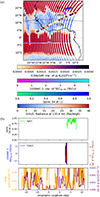 |
Figure 12 Similar to Figure 9 except for perturbed Event 2 on 2022-03-28 between 20:50-21:10 UTC. |
| In the text | |
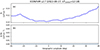 |
Figure 13 Same as Figure 5 for Track 15570 on 2022-08-17. |
| In the text | |
|
Figure 14 Same as Figure 2, except for the acquisition shown in top panel: (a) and (b) are for COSMIC-2 ionPrf Csm4 at 12:29 UTC, and bottom panel: (c) and (d) for Csm5 at 12:34 UTC. For both the profiles shown, the RO link is between Rx COSMIC-2 satellite C2E6 and Txs GPS PRNs (G26 and G20) on 2022-08-17. |
| In the text | |
|
Figure 15 (a) Solar activity level index F10.7 for the period under study, (b) Total number of COSMIC-2 ionPrfs and Spire conPhs files available per day via UCAR repository. |
| In the text | |
|
Figure 16 Statistics of scintillation or irregularities occurrence rates from COSMIC-2 and Spire data, for GPS constellation only over (a) African longitudinal, and (b) American longitudinal sectors. Data between ± 40° geographic latitudes and 1800 – 0300 LT have been used. |
| In the text | |
|
Figure S1: Daytime GOLD disk images from 135.6 nm wavelength (left panel) and LBH bands (right panel) on 2022-08-17. |
| In the text | |
|
Figure S2: Daytime GOLD disk images from 135.6 nm wavelength (left panel) and LBH bands (right panel) on 2022-03-28 |
| In the text | |
|
Figure S3: Map with different sensor measurements color-coded and overlaid on the GOLD’s daytime radiance image for quiet time event on 2022-08-17. C1 = Csm4 COSMIC-2 ionPrf, C2 = Csm5 COSMIC-2 ionPrf as described in Figure 14 of the main text, and ICON = ICON Track 15570 on 2022-08-17 as described in Figure 13 of the main text. |
| In the text | |
Current usage metrics show cumulative count of Article Views (full-text article views including HTML views, PDF and ePub downloads, according to the available data) and Abstracts Views on Vision4Press platform.
Data correspond to usage on the plateform after 2015. The current usage metrics is available 48-96 hours after online publication and is updated daily on week days.
Initial download of the metrics may take a while.