| Issue |
J. Space Weather Space Clim.
Volume 16, 2026
|
|
|---|---|---|
| Article Number | 9 | |
| Number of page(s) | 17 | |
| DOI | https://doi.org/10.1051/swsc/2026002 | |
| Published online | 21 April 2026 | |
Technical Article
Relativistic Electron and Proton Experiment for the HENON mission: simulated performance
1
Department of Physics and Astronomy, University of Turku, Turku, Finland
2
Aboa Space Research Oy (ASRO), Turku, Finland
3
National Institute for Astrophysics (INAF) – Institute for Space Astrophysics and Planetology (IAPS), Rome, Italy
* Corresponding author: This email address is being protected from spambots. You need JavaScript enabled to view it.
Received:
28
October
2025
Accepted:
30
January
2026
Abstract
HEliospheric pioNeer for sOlar and interplanetary threats defeNce (HENON) is a 12U CubeSat that will explore for the first time ever the Distant Retrograde Orbit in the Sun-Earth system, bringing a payload suited for Space Weather observations and science. Initially designed for the Foresail-2 nanosatellite mission, the Relativistic Electron and Proton Experiment (REPE) instrument has since evolved for deployment in a variety of future missions, including the HENON mission. REPE is a particle telescope developed to measure fluxes of high-energy electrons and protons over broad ranges of energies, relevant to the space radiation environment. The instrument is designed to measure electron energy spectrum from 0.1 to 10.4 MeV and proton energy spectrum from 2 to hundreds of MeV. We present Monte Carlo simulations of REPE performance using Geant4. We evaluate the performance in terms of sensitivity (geometric factor), energy resolution, and cross-contamination between measured species. We show that the instrument meets the scientific requirements of the mission.
Key words: Space radiation / Instrumentation / Monte Carlo simulations / Response functions
© C. Ngom et al., Published by EDP Sciences 2026
 This is an Open Access article distributed under the terms of the Creative Commons Attribution License (https://creativecommons.org/licenses/by/4.0), which permits unrestricted use, distribution, and reproduction in any medium, provided the original work is properly cited.
1 Introduction
Solar energetic particles (SEPs) constitute one of the most important elements of particle radiation environment in near-Earth interplanetary (IP) medium (Vainio et al., 2009). SEPs are emitted from the Sun in sporadic events associated with solar flares and fast coronal mass ejections (CMEs). Radiation effects on spacecraft electronics and crew are mainly caused by ions energetic enough to penetrate the spacecraft hull (some tens of MeV/nucleon depending on the thickness of the shielding). Protons of tens of MeV energies carry most of the total dose while protons of hundreds of MeV and heavy ions at tens of MeV/nucleon energies are the most important for causing single event effects (e.g., Duzellier, 2005; Dodd et al., 2010). Relativistic electrons, while not a major radiation risk in the IP space themselves, can be used to forecast the ion fluxes with some tens of minutes lead time (Posner, 2007; Laurenza et al., 2024; Stumpo et al., 2024; Posner et al., 2024; Dröge et al., 2025). High-quality measurements of relativistic electrons and ions in IP medium are, therefore, crucial for monitoring and forecasting the space radiation environment outside the shield provided by the Earth’s magnetosphere.
HEliospheric pioNeer for sOlar and interplanetary threats defeNce (HENON) (Cicalò et al., 2025; Provinciali et al., 2024) is a pioneering deep space 12U CubeSat mission aiming at realizing a quality leap in our capabilities to timely predict space weather effects as well as progressing in the understanding of space weather physical mechanisms. The HENON objectives are to:
provide constant monitoring of the radiation environment in deep space;
give quasi-real-time alerts of SEPs arrival at the Earth and geomagnetic storms, offering a 10 times improvement in the prediction lead time;
give useful scientific data to enhance our knowledge of Heliophysics. In addition, there are two important technological objectives, namely:
fly for the first time ever the Distant Retrograde Orbits (DROs), which have a critical importance also in other space contexts;
demonstrate reliability, availability and maintainability of the CubeSat technologies in deep space mission.
The Relativistic Electron and Proton Experiment (REPE) concept, initially developed for the Foresail-2 mission (Anger et al., 2023) by the University of Turku, was designed to characterize Earth’s radiation belts. It is configurable to fit various mission requirements, from low Earth orbit (LEO) to high Earth orbits and beyond. Following the standby of the Foresail-2 mission, the REPE instrument concept underwent significant modifications and improvements to meet the requirements of the HENON mission. REPE was tailored to measure high-energy electron and proton fluxes in deep space, enabling the study of space radiation beyond Earth’s immediate vicinity to provide data for space weather forecasting.
To evaluate the performance of REPE and demonstrate its ability to meet the scientific objectives of the mission, we conducted Monte Carlo simulations using the Geant4 toolkit (Agostinelli et al.,2003). In this paper, we present and discuss the results of these simulations, including the simulated energy and angular response functions of the instrument, as well as the cross-contamination between electrons and protons across the energy channels. Additionally, a bow-tie analysis was performed to obtain effective geometric factors and characteristic energies for the spectral channels of the instrument. Synthetic datasets representing past solar events were produced by combining simulated response functions with flux measurements from other instruments in previous missions, and later compared with the original datasets.
2 REPE instrument
REPE is a multi-detector particle instrument designed to measure high-energy electron and proton fluxes. REPE features a compact design with dimensions of 95 × 90 × 76 mm3 and a total mass of approximately 1.2 kg. Its design is specifically tailored for integration into lightweight and space-constrained missions, such as CubeSats. REPE requirements for the HENON mission are to measure fluxes with electron energy spectrum from 0.25 to 10.4 MeV and proton energy spectrum from 3 to 100+ MeV. For electrons, the energy resolution required is ΔE/E ≤ 40% at energies below 1 MeV and ΔE/E ≤ 80% at higher energies. For protons, the energy resolution required is ΔE/E ≤ 50% at energies below 70 MeV and ΔE/E ≤ 80% at higher energies. The detector boresight direction is perpendicular to the spacecraft spin axis to be able to determine the angular distribution of the particle fluxes in the spin plane.
2.1 Detector head
The detector unit (Fig. 1, left) consists of a stack of three silicon detectors (D1, D2, and D4) and one scintillator (D3) made of GAGG(Ce) – gadolinium aluminium gallium garnet (Gd3Al2Ga3O12) doped with cerium – combined with a photodiode that converts light signals to charge pulses. The Si detectors have a thickness of 300 μm. Their active areas (shown in dark blue in Fig. 1, right) increase from top to bottom of the stack: 3 × 7 mm2 for D1, 7 × 11 mm2 for D2, and 10 × 16 mm2 for D4. The scintillator is 10 mm thick, and the surface area is 10 x 16 mm2. The detector stack aperture is protected with a double layer of an aluminised (100 nm Al) Kapton foil (25 μm) to prevent low-energy radiation from entering the stack.
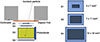 |
Figure 1 Schematic REPE detector stack cross section (left) and Si detectors areas (right), showing active regions in dark blue and passive regions in light blue. |
The D1, D2, and D4 are ion-implanted silicon detectors produced by Micron Semiconductor. Each detector has an aluminium coating and a dead layer of 500 nm total thickness on each side. The intrinsic noise of these detectors is about 10 keV FWHM equivalent energy deposit at room temperature.
The D3 is a scintillation detector coupled to a 10 × 10 mm2 photodiode produced from a 300 μm wafer. The intrinsic noise of the diode is similar to that of one of the silicon detectors. The measured energy resolution of the D3 scintillation detector is 7% at 662 keV. The overall detector energy efficiency is 9.7%, i.e., a 1 MeV deposit in the scintillator produces a signal equivalent to a 97 keV deposit in the silicon bulk.
The detector unit is connected to electronic boards, allowing detector biasing, signal amplification, and processing. Linear regulators are used to ensure low-noise power generation. The amplifier chain consists of a classical Junction Field Effect Transistor (JFET)-input preamplifier, followed by a differential amplifier. The amplifier chain is read out by a fast 14-bit analog-to-digital converter (ADC). The digitised pulses are further collected, filtered, and analysed using Field Programmable Gate Array (FPGA) logic.
2.2 Particle classification
When a particle is detected, it generates a signal from each detector recording a hit. Each of these detectors produces a specific part of the signal, corresponding to the energy deposited by the particle in that detector. The particle classifier processes the hit information and the pulse height directly related to the energy deposited by the particle from all the detectors. The particle classifier converts these pulse height values into the energy scale, calibrated to reflect the actual energy deposit. The classifier uses these energy values, in combination with the hit pattern and timing information, to identify the species of the particle, i.e., distinguish between protons and electrons. The particle classifier is composed of four distinct sub-classifiers (denoted PC1 to PC4), with the appropriate sub-classifier being selected based on the combination of hits detected. The combinations of hits and the corresponding sub-classifier selection are illustrated in Figure 2. The detected particles are categorized on the basis of their species and energy. Each sub-classifier sorts particles into its separate energy histograms.
 |
Figure 2 Hit combinations for the REPE particle classifier. Green colour denotes a hit in the detector, red colour denotes no hit, and blue colour denotes do not care if hit or no hit. All other hit combinations are to be counted as errors. |
PC1 classifies particles that stop in the D1 detector. These particles are classified either into electron, proton, or mixed electron-proton bins based on the measured deposited energy in D1. While a single energy deposit is not enough to conclusively determine the species, low energy deposits are more likely to be caused by electrons and high deposits by protons for particles stopping in the detector and not detected in D2. PC2 classifies particles that hit both detectors D1 and D2. It identifies the species using the standard ΔE–E method (Tassan-Got, 2002). The first detector (the ΔE detector) absorbs a fraction of the incident particle’s initial energy, while the second detector (the E detector) captures the remaining energy. The ΔE–E method enables identification of particle species based on the particle’s position on the ΔE–E plane, which reflects its energy loss characteristics as it passes through the two-detector system. After separating electrons and protons, the energies deposited in both detectors are summed, and the classification into energy channels is performed based on the total energy. PC3 classifies particles that hit detectors D2 and D3 regardless of whether there is a hit in D1 or not. This configuration is chosen because D1 has a significantly smaller active area compared to the other detectors. Particle identification is achieved using the ΔE–E method with the energy deposits in D2 and D3. The deposits in D2 and D3 detectors are then summed, and the classification into energy channels is performed based on this combined energy deposit. PC4 classifies particles that penetrate the whole detector stack, but does not care about a hit in D1. These particles are classified into proton bins based on the deposited energy in D2, D3, and D4. PC4 updates proton channels only, since electrons penetrating the whole detector stack would have such high energies that they would generally fall out of the targeted energy range of REPE. If these electrons are present in the environment, they would contaminate mainly the highest energy proton channels, as shown below.
To simplify the computation of the classification algorithm, we choose to base the identification of detected particles on their Particle Identification Number (PIN), which is calculated using the energy deposit data of the two-detector system by making use of the fact that the energy loss rate of the particle in the medium, −dE/dx, is roughly inversely proportional to the energy of the particle (see Sect. 3.2.1 below). Consequently, the particle classification decision is determined by the particle’s position on what we refer to as the PIN–E plane. This approach enables the identification of particles as either electrons or protons based on their PIN value, which must fall within a predefined range specific to each species. Since protons penetrate the entire detector stack in PC4 and therefore lose only part of their energy in the telescope, the PIN–E method is not applicable. Instead, PC4 identifies detected protons by measuring the energy deposit in the scintillator D3. The energy losses in D2 and D4 are used to provide information on the propagation direction of protons penetrating the stack at energies close to the penetration threshold. The classifier energy channels boundaries are quasi-logarithmically spaced (see Appendix A). The electron channels are denoted from E1 to E16, the proton channels are denoted from P1 to P22, and the mixed electron-proton channels are denoted PE1 and PE2.
3 Geant4 simulations
3.1 Model
The geometric factor for a complex multi-element telescope such as the REPE instrument is typically calculated using a Monte Carlo simulation (Oleynik, 2021b; Liu et al., 2022; Oleynik et al., 2020a,b). This technique involves simulating a large number of particle trajectories to determine the instrument’s response to incoming particles. Following the methodology proposed by Sullivan (1971), we used the Geant4 simulation toolkit (Agostinelli et al., 2003; Allison et al., 2006) to estimate the REPE response to protons and electrons. The simulation is based on a realistic three-dimensional (3D) digital model of the REPE instrument shown in Figure 3. The left panel shows the detector stack, topped with the Kapton foil and collimator structure, without electronic boards, fasteners, and the rear section of the outer mechanical structure, while the right panel presents the complete REPE assembly positioned inside a spherical radiating source. The model utilises the Geometry Description Markup Language (GDML) (Chytracek et al., 2006) and incorporates all mechanical structures, excluding electronic components and wiring. We created the model for Geant4 simulations by converting the 3D mechanical model to GDML using Pyg4ometry software (Walker et al., 2022). The simulation is done without incorporating the satellite structures to isolate the response of REPE itself. The model is placed inside a cubic World volume, filled with G4_Galactic (space vacuum).
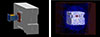 |
Figure 3 REPE mechanical model visualized in Geant4 from the GDML file. Left: Detector stack inside REPE, right-to-left: the Kapton foil and collimator, D1, D2, scintillator D3, and the D4 detector, shown without the electronic boards and the rear mechanical structure. Right: REPE model placed inside a spherical radiating source within the World volume. |
The source of incident particles is modelled as a radiating sphere with an 8 cm radius, completely surrounding the instrument. The initial positions of particles are randomly assigned according to a uniform distribution across the sphere’s surface. The angular distribution of the particles is defined so that the flux distribution follows the cosine law (Greenwood, 2002) with respect to the sphere surface normals. This approach ensures an exposure for an accurate determination of the response function. The instrument’s performance has been simulated across a wide range of particle energies relevant to space radiation environments. The simulated particle flux follows an isotropic and flat energy spectrum within the energy ranges of 30 keV to 30 MeV for electrons and 1 MeV to 1 GeV for protons. The particle interactions are modelled using the QGSP_BERT physics list, which combines the Quark-Gluon String model (QGSP) for high-energy hadronic processes with the Bertini Cascade model (BERT) for accurate low- and intermediate-energy interactions. Additionally, the Electromagnetic (EM) Physics Option 3 is incorporated to enhance the precision of photon and charged particle transport simulations. The version of the tool is Geant4-11.2.1.
For numerical and computational reasons, the Monte Carlo simulations were conducted in discrete energy intervals for both protons and electrons. Within each interval, primary particles were generated with a uniform energy distribution, and the results from all intervals were subsequently combined to represent a flat spectrum over the entire energy range. For protons, 32 independent runs were performed per interval. A total of 2 × 10⁹ primary protons were simulated per run in the 1–3 MeV, 3–10 MeV, and 10–30 MeV energy ranges. For the 30–100 MeV and 100–300 MeV ranges, each run included 1 × 10⁹ primary protons, while the highest range (300–1000 MeV) used 5 × 10⁸ primary protons per run. For electrons, 64 runs were performed for each defined interval. The 0.03–0.1 MeV and 0.1–0.3 MeV ranges used 2 × 10⁹ primary electrons per run. The subsequent energy ranges—0.3–1 MeV, 1–3 MeV, and 3–10 MeV – each included 1 × 10⁹ primary electrons per run. In the highest interval (10–30 MeV), 5 × 10⁸ primary electrons were simulated per run. These numbers of primary particles were chosen to maximize statistical accuracy while remaining within the computational limits of Geant4.
The Geant4 simulation (Oleynik, 2021a) produces tables of recorded energy deposits in the sensitive detectors. Further, the energy deposit histograms for the classifier coincidence conditions are generated. To achieve this, we opted to collect raw data from the sensitive detectors, saved in .root files, and perform the post-processing separately using scripts written in Python. This approach allows for tuning the REPE particle classifier by adjusting the accumulation method for energy bins in histograms, even after the simulation has been completed, without the need to rerun the entire simulation. Subsequently, the REPE instrument response is calculated taking into account the particle identification process when applicable, using the PIN calculated in PC2 and PC3, as well as the energy loss in the scintillator D3 in PC4.
3.2 Results
3.2.1 Particle identification
The Particle Identification Number (PIN) in MeV2 is calculated for PC2 and PC3 based on the following equation:
 (1)
(1)
with ΔE the energy deposit in ΔE detector (ED1 in PC2 and ED2 in PC3) and E is the total energy of the particle deposited in the two layers included in the analysis (ED1 + ED2 in PC2 and ED2 + ED3 in PC3).
The PIN–E plots for electrons and protons are presented in Figure 4. For both PC2 and PC3, we observe that the majority of detected protons align along an almost straight and constant line within a PIN ∈ [20, 50] MeV2, whereas most detected electrons are positioned well below these proton values. This distinction enables us to define the appropriate PIN ranges for particle discrimination. For PC2 the ranges are PIN ∈ [0.01, 1] MeV2 for electrons and PIN ∈ [10, 100] MeV2 for protons. For PC3 the ranges are PIN ∈ [0.01, 10] MeV2 for electrons and PIN ∈ [10, 100] MeV2 for protons. The selected PIN range is represented by the white rectangles. PIN values outside the electron and proton ranges are counted as errors.
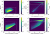 |
Figure 4 Particle Identification Number (PIN) as a function of energy deposited in: D2 for electron for PC2 (top left), D2 for proton for PC2 (top right), D3 for electron for PC3 (bottom left), and D3 for proton for PC3 (bottom right). |
The energy deposited by protons in D3 as a function of the energy loss ratio between D2 and D4, ED2/(ED2 + ED4), is shown in Figure 5. Protons entering through the collimator aperture lose more energy in D4 than in D2 due to the increase in linear energy transfer (LET) with distance travelled, reaching its maximum at the Bragg peak (Bragg, 1904; Bragg & Kleeman, 1905). Likewise, backwards-penetrating protons deposit more energy in D2 than in D4. For proton energies near the threshold required to traverse the entire detector stack, we distinguish the direction of the incoming protons by analysing the energy ratio between D2 and D4. The directional separation is performed with the following conditions:
Forward incidence: ED2/(ED2 + ED4) < 0.5.
Backward incidence: ED2/(ED2 + ED4) > 0.5.
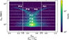 |
Figure 5 Energy loss in D3, the scintillator, as a function of energy deposit ratio between D2 and D4 with PC4 proton channels represented. |
Based on this criterion, we classify them into separate channels. Channels P15 and P16 register protons arriving from the aperture, while channels P21 and P22 record backwards-penetrating protons. The remaining channels detect protons from both directions. Since the energy deposited in D3 is significantly lower than the total incident energy of the protons, PC4 is configured with energy-loss channels rather than absolute energy channels. The energy loss (dE/dx) in D3 is approximately inversely proportional to β2. Since β2 is proportional to the kinetic energy, dE/dx becomes roughly inversely dependent on the particle’s kinetic energy (Jackson, 1998). This relationship enables us to convert the energy-loss channels into energy channels on the ground.
3.2.2 Energy channels’ response functions
The geometric factor G [cm2 sr] (generalized as the response function of an instrument) is the factor of proportionality relating the counting rate C [s−1] to the incident (mono-energetic and isotropic) particle flux I0 [cm−2 sr−1 s−1],
 (2)
(2)
When the flux depends on the incident particle energy, E, we typically use the (isotropic) response function, R(E) [cm2 sr], of a counting channel to compute the counting rate as
 (3)
(3)
where dI/dE [cm−2 sr−1 s−1 MeV−1] is the differential (isotropic) intensity. The simulated response functions (Sullivan, 1971) of the REPE instrument channels are derived from the Geant4 data using the following equation:
 (4)
(4)
where Nd(E) is the number of particles (of incident energy E) detected, N0(E) is the total number of particles simulated, and π · A0 is the geometric factor of a radiating sphere of area A0.
The response function of REPE electron channels is presented in Figure 6. REPE detection threshold for electrons starts at an energy slightly lower than 200 keV. PC1 and PC2 combined cover low energy channels up to 1 MeV, whereas PC3 allows covering higher energy channels starting from 600 keV up to 30 MeV. PC1 and PC2 electron channels present a differential response in the nominal energy range, except the last one (E7), which presents integral characteristics. The curves present a rise of the geometric factor at higher energies. PC3 electron channels have integral characteristics and present higher geometric factors due to the larger field of view, since a hit is not required in detector D1, and the collimator starts to be partly transparent at the highest energies. Additionally, the channels exhibit a shift in their response function of approximately 100 keV, resulting from the energy deposited in D1 that is not included in the total energy computation. The energy resolution for electron channels varies between 27 and 37%.
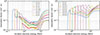 |
Figure 6 Electron energy channels response functions, and PE channels response functions with electron contribution. Left: PC1 and PC2, Right: PC3. |
Figure 7 shows the response function of REPE proton channels. REPE detects protons starting from an energy of 2 MeV. PC1 and PC2 together cover low-energy channels up to 11 MeV, while PC3 covers higher-energy channels from 9 MeV up to 90 MeV. Proton channels in PC1, PC2, and PC3 are differential, most of them presenting a boxcar-like shape of their response in the nominal energy range. They present a rebound at high energies E ≥ 40 MeV. PC3 channels present higher geometric factors for the same reason as observed with electrons. Except for P14, the channels also show a shift in their response function from approximately 3.5 MeV for P7 to around 1 MeV for P13 due in part to the energy deposited in D1 that is not included in the total energy calculation. The resolution for proton energy channels in PC1, PC2, and PC3 vary between 9% and 30%.
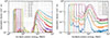 |
Figure 7 Proton energy channels response functions and PE channels response functions with proton contribution. Left: PC1 and PC2, Right: PC3. |
PC4 channels’ response functions are presented in Figure 8. The penetrating protons are detected with an energy threshold of 70 MeV. The response functions of the energy-loss channels are nicely differential at incident energies up to around 400 MeV, then tend to become more integral-like at higher energies. The resolution of the PC4 channels remains below 37% up to 300 MeV and below 70% up to 800 MeV. Detailed values of the channel resolutions are presented in Appendix B. All channels of the REPE instrument, except the electron channels from E3 to E7, exhibit a sufficient geometric factor exceeding 0.1 cm2 sr, including the penetrating proton channels. However, when combined, channels E3 and E5 (with identical nominal energy ranges) also achieve a geometric factor of 0.1 cm2 sr.
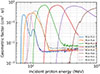 |
Figure 8 PC4 proton energy-loss channels response functions. Channels P15 and P16, which detect protons entering through the aperture, and channels P16–P20, sensitive to protons from both directions are plotted with solid lines. Channels P21 and P22 recording backward-penetrating protons are presented in dashed lines. |
3.2.3 Cross-species contamination of the channels
Cross-contamination of instrument channels by misclassified particle species can affect flux measurement accuracy and needs to be analyzed to implement correction techniques in data analysis. Figure 9 shows electron channels’ sensitivity to protons and inversely proton channels’ sensitivity to electrons. The inset on the left panel provides a zoomed view of the x-axis in the energy range between 1.8 and 3 MeV. PC1 electron channels experience high contamination from low-energy protons E ≤ 3 MeV, with contamination levels on the same order of magnitude as the nominal response. Other electron channels exhibit relatively low contamination from low-energy protons. PC2 proton channels remain unaffected by electrons up to 30 MeV, ensuring clean proton fluxes measurements. In the same way, the PC1 and PC3 channels are free from electron contamination up to 10 MeV.
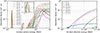 |
Figure 9 Cross-contamination geometric factors of REPE energy channels. Left: Electron channels response to protons. Right: Proton channels response to electrons. |
3.2.4 Angular sensitivity
The sensitivity of the instrument varies with the incident angle and energies of the particles, which influences the classification and the response characteristics. The angular response for three electron and three proton energy ranges, i.e., low, intermediate, and high energies, is shown in Figure 10. The energy range values are [0.1, 1] MeV, [1, 3] MeV, [3, 10] MeV for electrons and [1, 10] MeV, [10, 70] MeV, [70, 1000] MeV for protons. The white contour lines represent 50% of the peak response level.
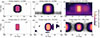 |
Figure 10 Geometric factor of REPE instrument as a function of particle the incident zenith (theta) and azimuth (phi) angles for three electron and proton energy ranges. The white contour lines represent 50% of the peak response level. Top: electron, Bottom: proton. |
At low energies, the particles are mainly classified in PC1 and PC2. We observe that the instrument shows almost similar behaviour for electrons and protons with slightly different response level. The electron field of view extends slightly beyond the collimator aperture, whereas the proton field of view remains well confined within the aperture boundaries. The 50% response level occurs at an azimuth angle of approximately 50° width.
For intermediate energies, the particles are mainly classified in PC3. For both electron and proton, the instrument demonstrates a broader field of view due to the non-necessity of a hit in detector D1 and the increasing transparency of the collimator. Additionally, the response is slightly influenced by particles incident from the backward direction. The asymmetry observed for protons arises from the azimuthal design asymmetry of the instrument (see Fig. 3, right), which results in non-uniform shielding between the two sides of the detector. The 50% response level shifts to an azimuth angle of around 40° width.
At high energies, the electrons are classified in PC3, whereas the protons are classified in PC4. The collimator transparency further increases, affecting electron detection by allowing more backwards-travelling electrons to be registered. In contrast, the proton field of view remains relatively well constrained to the aperture in both forward and backward directions. As with intermediate energies, the 50% response level stabilizes at an azimuth angle of about 40° width.
3.2.5 Bow-tie analysis
A bow-tie analysis (Van Allen et al., 1974) was performed on the instrument channels to determine the specific effective energy where the geometric factor of a particle channel remains the least dependent on the incident energy spectrum. This allows us to convert the counting rate, C, to intensity, dI/dE ≡ f(E), using
 (5)
(5)
where GδE is the effective differential geometric factor for the counter channel. The best results are achieved when realistic spectral forms are used when deriving the geometric factors and effective energies.
The response function of each channel has been folded with power-law spectra of the form f(E) = A × Eα, where the spectral index α varies from −4 to −2, representing the expected range observed by the instrument (Guo et al., 2019; Kühl et al., 2016). The effective geometric factor for differential channels is calculated based on the following formula (Oleynik, 2021b):
 (6)
(6)
where R(E) is the response function of the channel, and Eeff is the corresponding effective energy for a given spectrum f(E). For integral channels, the calculation is based on the following formula (Oleynik, 2021b):
 (7)
(7)
where G(Et) is the effective geometric factor, and Et is the effective threshold energy of the energy channel. For the power-law spectra applied (and assuming that α < −1), these become
 (8)
(8)
and
 (9)
(9)
respectively.
Figure 11 shows the bow-tie for the differential proton channel P8 formed by the family of GδE function plots calculated for the applied range of power-law indices α ∈ [−4, −2]. The optimal effective geometric factor and effective energy Eeff for this channel are located at the neck of the bow-tie, where the geometric factor exhibits the minimum standard deviation across the considered spectral indices, thus yielding the lowest systematic uncertainty of the factor. In other words, if we use the Eeff to characterize an instrument channel when measuring a power-law incident energy spectrum, the uncertainty is minimal. The effective geometric factor and effective energy values of all electron and proton channels are available in Appendix C. A bow-tie analysis was also carried out for the cross-species contamination, and the corresponding values are available in Appendix D.
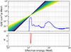 |
Figure 11 Bow-tie analysis using model spectra with a range of indices α from −4 to −2 and response function in cm2 sr (blue line) of the P8 proton channel. The lower panel shows the statistical measure of the bow-tie spreading in standard deviation units normalized to the deviation of GδE at Eeff for the channel. |
3.2.6 Synthetic data
We calculated synthetic fluxes in REPE channels for November 1–17, 1997, during which several SEP events occurred, including one ground-level enhancement (GLE 55) on November 6. The GLE is produced by an SEP event in which particles reach relativistic energies, and it is usually associated with high intensities at lower energies. Synthetic electron fluxes are based on SOHO/EPHIN observations and proton fluxes on the SEPEM reference dataset v3.2. In addition, we have included quiet-time solar proton fluxes from (Valtonen et al., 2001) and galactic cosmic ray (GCR) fluxes calculated using the force-field approximation (Gleeson & Axford, 1968; Usoskin et al., 2005) with the local interstellar spectrum (LIS) from (Vos & Potgieter, 2015) and daily modulation potential from (Väisänen et al., 2023).
We cleaned the EPHIN electron channel fluxes by replacing any fluxes ten times higher than the median of a moving 13-point centred window with the median. Then, we applied smoothing by calculating moving averages with different window lengths ranging from 12 hours to 1 minute and calculating a weighted sum of those averages, where the weight depends on the flux level. The SEPEM v3.2 proton dataset is already pre-processed and background-subtracted, and therefore we only resampled the SEP proton fluxes to one-minute resolution and applied the smoothing with window lengths ranging from 4 h to 3 min. To reintroduce the background for protons, quiet-time solar proton and galactic cosmic ray proton fluxes were added to the time series.
The processed electron and proton spectra were then interpolated (and extrapolated) to a fine energy grid (between 30 keV to 30 MeV for electrons and 1 MeV to 1 GeV for protons) at each timestep. Next, the interpolated spectra were multiplied by the response function of each electron and proton channel, and the products were integrated over the energy range. Intermediate counts were then calculated by multiplying by the duration of one REPE measurement period, which was assumed to be 30 s. Final REPE counts were sampled from the Poisson distribution, taking the intermediate counts as means for each time step and channel. Finally, synthetic fluxes were calculated by dividing the counts by the channel geometric factors from the bow-tie analysis. It should be noted that during periods without SEP activity, the majority of the proton energy range covered by REPE is dominated by the increasing part of the GCR spectrum, and therefore, the bow-tie-derived channel energies and geometric factors are not representative. For SEP periods, the fluxes calculated with bow-tie results are accurate, and without the need for complex calculations, they could be included in onboard data processing.
Figures 12 and 13 present examples of the synthetic electron and proton fluxes, calculated for November 1–17, 1997, at two time resolutions for REPE (30-s and 5-min). The top panels present electron channels E3, E10, and E13 (in blue, orange, and green, respectively) along with 1-minute EPHIN fluxes interpolated to the same energies (in light green, purple, and light blue, respectively). The difference between REPE E3-channel and EPHIN during November 5-6 can be attributed to proton contamination. Similarly, the bottom panels present proton channels P4, P11, and P19 (in blue, orange, and green, respectively) along with SEPEM fluxes at 1-minute resolution interpolated to the same energies. Here, some contamination-related differences can be seen in the highest energy channel around the beginning of November 7.
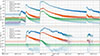 |
Figure 12 Synthetic electron (top panel) and proton (bottom panel) fluxes for November 1–17, 1997. Time resolution is 30 seconds for REPE. |
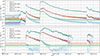 |
Figure 13 Synthetic electron (top panel) and proton (bottom panel) fluxes for November 1–17, 1997. Time resolution is 5 min for REPE. |
Synthetic electron (top panel) and proton (bottom panel) fluxes for November 1–17, 1997. Time resolution is 5 min for REPE.
4 Discussion
The present study provides an assessment of the REPE instrument over various performance criteria regarding the scientific requirements for the HENON mission. The results demonstrate that REPE satisfies, and in some aspects exceeds, the scientific requirements for the HENON mission.
The instrument covers a larger energy range than required, extending beyond 10 MeV for electrons and up to 1000 MeV for protons. This extended capability enhances the instrument’s potential to monitor high-energy events. REPE has well-defined energy channels: six differential channels for electrons up to approximately 6 MeV and ten integral channels, as well as twenty-one differential channels for protons up to approximately 400 MeV and two integral channels. The instrument presents a high resolution of energy channels with ΔE/E < 40% for electrons up to 10 MeV and protons below 70 MeV, allowing the analysis of the spectrum with good accuracy. The geometric factor is sufficiently high, exceeding 0.1 cm2 sr even for high-energy penetrating particles, despite the relatively small detector size. This ensures a sufficient particle counting statistic for the flux measurements during large solar events.
REPE is able to identify whether the particle is an electron or a proton with a certain level of accuracy, which has been evaluated by analysing the channel cross-contamination. The results indicate that proton channels are not contaminated by electrons of energy lower than 10 MeV, and most electron channels experience a negligible contamination by protons. This ensures reliable measurements of electron and proton fluxes across the energy range of interest with minimal influence from the other species. The potential contamination from unwanted particles such as alpha particles and heavy ions has not yet been evaluated. However, we expect the PIN–E analysis to be able to separate protons and heavier ions very well, so the potential contamination from these ion species is likely to be in PC1 channels only. The angular response is satisfactory for low-energy electrons and low- and high-energy protons. The instrument is capable of measuring the azimuth angle distribution with an angular resolution of approximately 40° meeting the 45° requirement of the HENON mission.
We used bow-tie analysis to determine the optimal effective geometric factor and effective energy for each channel. These results were used to generate synthetic fluxes measurement of the November 1–17, 1997 events. The comparison of the synthetic spectra of the REPE instrument with EPHIN and SEPEM spectra shows a relatively good agreement overall at high particle fluxes for both electrons and protons. The results show a limitation of the REPE instrument in accurately measuring low relativistic electron fluxes, which may be attributed to its smaller geometric factor compared to EPHIN and to its lack of a full anti-coincidence shield capable of vetoing minimally ionizing cosmic-ray protons that penetrate all the passive shielding. Due to its smaller geometric factor compared to EPHIN, however, REPE is capable of accurately measuring high fluxes without significant saturation. For protons, the cosmic-ray background does not constitute a similar problem, but the small geometric factor limits the clear detection of solar protons in weaker events at high time resolution. This will have to be tackled by using longer integration times than 30 seconds, as was demonstrated by the use of 5-minute resolution above, showing that the event on November 4, 1997, below the GLE range could be detectable up to ∼450 MeV.
The REPE electron fluxes in the energy range from 0.25 to 10.4 MeV will be used in the SEP forecasting method that will run in real time on board HENON. The high energy resolution of the REPE combined with the good particle discrimination allow the HENON mission to provide a better spectral analysis of deep space during SEP events with a more accurate energy distribution of particles. The wide energy coverage allows to capture rare high-energy events. The REPE geometric factor is sufficient to provide high counting capability, allowing the measurement of high particle fluxes during SEP events. The angular resolution further allows to study particle anisotropies – a capability that is missing from several other missions in IP space.
Some further refinements of the modelling would allow to enhance the accuracy of the results. The total light output generated by a particle in the GAGG scintillator experiences quenching phenomenon, also known as Birks effect (Birks, 1964), when the ionization density increases. For electrons, this non-linearity between the energy deposit and the pulse height remains negligible as the linear energy transfer is low. However, this phenomenon can be significant for protons (Furuno et al., 2021) but was not corrected in the present simulation, introducing uncertainties in the response functions. We will investigate this further after experimental determination of the quenching effects of our scintillators. The simulations were done without the satellite model providing the REPE instrument characteristics itself. Incorporating the satellite’s mass distribution will impact the channels’ geometric factors, particularly for the backward proton channels, and consequently affect the measured count rates.
5 Conclusions
In this paper, we have performed a detailed simulation study of the REPE instrument designed to measure energetic particle radiation aboard the HENON mission. We have evaluated and presented the response functions of the spectral counting channels of the instrument based on detailed Geant4 modelling. REPE will be measuring protons over a broad energy range (from ∼2 to >500 MeV) and electrons from near-relativistic to ultra-relativistic energies (∼200 keV to ∼10 MeV).
We have demonstrated that the performance requirements of the instrument for the HENON mission can be fulfilled by the REPE design. Experimental data on instrument performance, validating the simulation modelling, will be obtained through calibration campaigns on ground and in space and will be reported in future studies. We will address the remaining idealities of the simulation modelling in those studies as well.
Acknowledgments
We gratefully acknowledge the use of SOHO/EPHIN electron observations as input to our simulation studies. SOHO is an international project of collaboration between ESA and NASA. We also acknowledge the use of ESA’s SEPEM Reference Data Set version 3.0 (produced under the following ESA Contracts: 20162/06/NL/JD; 4000108377/12/NL/AK; 4000107025/12/NL/AK; 4000115930/15/NL/HK, 4000127129/19/NL/HK, 4000127282/19/NL/IB/gg). We acknowledge the Heliospheric Pioneer for Solar and Interplanetary Threats Defence (HENON) mission Phase A/B and C. HENON is part of the Italian Space Agency (ASI) program Alcor and is being developed under the European Space Agency General Support Technology Programme (ESA-GSTP) through the support of the national delegations of Italy (ASI), UK, Finland, and the Czech Republic. The views expressed herein can in no way be taken to reflect the official opinion of ESA. M.F.M. and M.L. acknowledge the Space It Up project of ASI and the Ministry of University and Research, MUR, contract n. 2024-5-E.0 – CUP n. I53D24000060005. The work in the University of Turku was carried out under the umbrella of Finnish Centre of Excellence in Research of Sustainable Space (FORESAIL, Research Council of Finland, decision 352847). We gratefully acknowledge also the Proof of Concept funding from the Research Council of Finland (RADICS, decision 359530). The editor thanks Fan Lei and an anonymous reviewer for their assistance in evaluating this paper.
Conflict of interest
The authors declare no conflict of interest.
Data availability statement
The simulation data is available from the authors through reasonable requests.
References
- Agostinelli, S, Allison J, Amako K, Apostolakis J, Araujo H, et al. 2003. Geant4 – a simulation toolkit. Nucl. Instrum. Methods Phys. Res. A., 506(3): 250–303. https://doi.org/10.1016/S0168-9002(03)01368-8. [CrossRef] [Google Scholar]
- Allison, J, Amako K, Apostolakis J, Araujo H, Arce Dubois P, et al. 2006. Geant4 developments and applications. IEEE Trans Nucl Sci 53(1): 270–278. https://doi.org/10.1109/TNS.2006.869826. [CrossRef] [Google Scholar]
- Anger, M, Niemelä P, Cheremetiev K, Clayhills B, Fetzer A, et al. 2023. Foresail-2: space physics mission in a challenging environment, Space Sci. Rev. 219(8): 66. https://doi.org/10.1007/s11214-023-01012-7. [Google Scholar]
- Birks, JB. 1964. The scintillation process in alkali halide crystals. IEEE Trans. Nucl. Sci. 11(3): 4–11. https://doi.org/10.1109/TNS.1964.4323396. [Google Scholar]
- Bragg, WH. 1904. LXXIII. On the absorption of α rays, and on the classification of the # rays from radium. London Edinburgh Philos. Mag. J. Sci. 8(48): 719–725. https://doi.org/10.1080/14786440409463245. [Google Scholar]
- Bragg, WH, Kleeman R. 1905. XXXIX. On the α particles of radium, and their loss of range in passing through various atoms and molecules. London Edinburgh Philos. Mag. J. Sci. 10(57): 318–340. https://doi.org/10.1080/14786440509463378. [Google Scholar]
- Chytracek, R, Mccormick J, Pokorski W, Santin G. 2006. Geometry description markup language for physics simulation and analysis applications. IEEE Trans. Nucl. Sci. 53(5): 2892–2896. https://doi.org/10.1109/TNS.2006.881062. [CrossRef] [Google Scholar]
- Cicalò, S, Alessi EM, Provinciali L, Amabili P, Saita G, et al. 2025. Mission analysis for the HENON CubeSat mission to a large Sun–Earth distant retrograde orbit. Astrophys Space Sci 370(8): 83. https://doi.org/10.1007/s10509-025-04473-0. [Google Scholar]
- Dodd PE, Shaneyfelt MR, Schwank JR, Felix JA. 2010. Current and future challenges in radiation effects on CMOS electronicsIEEE Trans. Nucl. Sci. 57(4):1747–1763. https://doi.org/10.1109/TNS.2010.2042613. [Google Scholar]
- Dröge, H, Heber B, Karavolos M, Kollhoff A, Kühl P, Malandraki O, Posner A. 2025. The STEREO REleASE system: solar energetic proton forecasting in the heliosphere. Space Weather 23(6): e2025SW004434. https://doi.org/10.1029/2025SW004434. [Google Scholar]
- Duzellier, S. 2005. Radiation effects on electronic devices in space. Aerospace Sci. Technol. 9(1): 93–99. https://doi.org/10.1016/j.ast.2004.08.006. [Google Scholar]
- Furuno, T, Koshikawa A, Kawabata T, Itoh M, Kurosawa S, Morimoto T, Murata M, Sakanashi K, Tsumura M, Yamaji A. 2021. Response of the GAGG(Ce) scintillator to charged particles compared with the CsI(Tl) scintillator. J Instrum 16(10), P10012. https://doi.org/10.1088/1748-0221/16/10/p10012. [Google Scholar]
- Gleeson, LJ, Axford WI. 1968. Solar modulation of galactic cosmic rays. Astrophys. J. 154: 1011. https://doi.org/10.1086/149822. [CrossRef] [Google Scholar]
- Greenwood, J.. 2002. The correct and incorrect generation of a cosine distribution of scattered particles for Monte-Carlo modelling of vacuum systems. Vacuum, 67(2): 217–222. https://doi.org/10.1016/S0042-207X(02)00173-2. [NASA ADS] [CrossRef] [Google Scholar]
- Guo, J, Wimmer-Schweingruber RF, Wang Y, Grande M, Matthiä D, Zeitlin C, Ehresmann B, Hassler DM. 2019. The pivot energy of solar energetic particles affecting the martian surface radiation environment. Astrophys. J. Lett. 883(1): L12. https://doi.org/10.3847/2041-8213/ab3ec2. [Google Scholar]
- Jackson, JD. 1998. Classical electrodynamics (3 edn). Hoboken, New Jersey, USA: John Wiley & Sons, Inc. [Google Scholar]
- Kühl, P, Dresing N, Heber B, Klassen A. 2016. Solar energetic particle events with protons above 500 mev between 1995 and 2015 measured with SOHO/EPHIN. Solar Phys. 292(1): 10. https://doi.org/10.1007/s11207-016-1033-8. [Google Scholar]
- Laurenza, M, Stumpo M, Zucca P, Mancini M, Benella S, Clark L, Alberti T, Marcucci MF. 2024. Upgrades of the ESPERTA forecast tool for solar proton events. J. Space Weather Space Clim. 14: 8. https://doi.org/10.1051/swsc/2024007. [Google Scholar]
- Liu J, Zhang Z, Liu Y, Zhao B, Wang R, Luo B, Liu S. 2022. Monte Carlo simulations of space particle detector onboard the CX-12(01) Satellite. In: 2022 International Conference on Sensing, Measurement & Data Analytics in the era of Artificial Intelligence (ICSMD), pp. 1–3. https://doi.org/10.1109/ICSMD57530.2022.10058423. [Google Scholar]
- Oleynik, P. 2021a. Instrument-Simulation software based on Geant4 framework. Available at https://github.com/phirippu/instrument-simulation. [Google Scholar]
- Oleynik, P. 2021b. Particle observations in near-earth space: design and verification of particle instruments for CubeSat experiments. PhD thesis, University of Turku, Turku, Finland. Available at https://urn.fi/URN:ISBN:978-951-29-8705-4. [Google Scholar]
- Oleynik, P, Vainio R, Hedman H-P, Punkkinen A, Punkkinen R, et al. 2020. Particle telescope aboard FORESAIL-1: Simulated performance. Adv. Space Res. 66(1): 29–41. https://doi.org/10.1016/j.asr.2019.11.010. [Google Scholar]
- Oleynik, P, Vainio R, Punkkinen A, Dudnik O, Gieseler J, et al. 2020. Calibration of RADMON radiation monitor onboard Aalto-1 CubeSat. Adv. Space Res 66(1): 42–51. https://doi.org/10.1016/j.asr.2019.11.020. [Google Scholar]
- Posner A. 2007. Up to 1-hour forecasting of radiation hazards from solar energetic ion events with relativistic electrons. Space Weather 5(5): 05001. https://doi.org/10.1029/2006SW000268. [Google Scholar]
- Posner A, Malandraki OE, Karavolos M, Tziotziou K, Smanis F, Heber B, Dröge H, Kühl P, Veldes GP. 2024. HESPERIA REleASE+: Improving solar proton event forecasting by means of automated recognition of type-III radio bursts. Space Weather 22(12):2024SW004,013. https://doi.org/10.1029/2024SW00401310.22541/essoar.171926580.08698491/v1. [Google Scholar]
- Provinciali L, Calcagno D, Amabili P, Saita G, Riccobono D, et al. 2024. HENON – Main challenges of a space weather alerts CubeSat Mission. In: 2024 IEEE Aerospace Conference, pp. 1–12. https://doi.org/10.1109/AERO58975.2024.10521299. [Google Scholar]
- Stumpo, M, Laurenza M, Benella S, Marcucci MF. 2024. Predicting the energetic proton flux with a machine learning regression algorithm. Astrophys. J. 975(1): 8. https://doi.org/10.3847/1538-4357/ad7734. [Google Scholar]
- Sullivan, J. 1971. Geometric factor and directional response of single and multi-element particle telescopes. Nuclear Instrum. Methods 95(1): 5–11. https://doi.org/10.1016/0029-554X(71)90033-4. [Google Scholar]
- Tassan-Got, L. 2002. A new functional for charge and mass identification in ΔE–E telescopes. Nuclear Instrum. Methods Phys. Res. B, 194(4): 503–512. https://doi.org/10.1016/S0168-583X(02)00957-6. [Google Scholar]
- Usoskin IG, Alanko-Huotari K, Kovaltsov GA, Mursula K. 2005. Heliospheric modulation of cosmic rays: Monthly reconstruction for 1951–2004. J. Geophys. Res. Space Phys. 110(A12): A12108. https://doi.org/10.1029/2005JA011250. [NASA ADS] [CrossRef] [Google Scholar]
- Vainio, R, Desorgher L, Heynderickx D, Storini M, Flückiger E, et al. 2009. Dynamics of the Earth’s particle radiation environment. Space Sci. Rev., 147(3–4): 187–231. https://doi.org/10.1007/s11214-009-9496-7. [CrossRef] [Google Scholar]
- Väisänen P, Usoskin I, Kähkönen R, Koldobskiy S, Mursula K. 2023. Revised reconstruction of the heliospheric modulation potential for 1964–2022. J. Geophys. Res. Space Phys. 128(4): e2023JA031352. https://doi.org/10.1029/2023JA031352. [Google Scholar]
- Valtonen, E, Kecskeméty K, Kunow H, Müller-Mellin R, Torsti J. 2001. Background reduction for quiet time particle fluxes aboard the solar and heliospheric observatory. J. Geophys. Res. 106(A6): 10705–10714. https://doi.org/10.1029/1999JA000456. [Google Scholar]
- Van Allen, JA, Baker DN, Randall BA, Sentman DD. 1974. The magnetosphere of Jupiter as observed with Pioneer 10: 1. Instrument and principal findings. J. Geophys. Res. 79(25): 3559–3577. https://doi.org/10.1029/JA079i025p03559. [Google Scholar]
- Vos, EE, Potgieter MS. 2015. New modeling of galactic proton modulation during the minimum of solar cycle 23/24. Astrophys. J. 815(2): 119. https://doi.org/10.1088/0004-637X/815/2/119. [NASA ADS] [CrossRef] [Google Scholar]
- Walker, S, Abramov A, Nevay L, Shields W, Boogert S. 2022. Pyg4ometry: a Python library for the creation of Monte Carlo radiation transport physical geometries. Comput. Phys. Commun. 272: 108228. https://doi.org/10.1016/j.cpc.2021.108228. [Google Scholar]
Appendix A: REPE energy channels
Table A1 presents the electron and proton energy channels of the particle classifier according to the deposited energy ranges and detector combinations. The channel’s energy intervals are defined between columns E1 and E2 (in keV). Each configuration represents a different combination of hits: PC1: Energy deposited only in detector D1. PC2: Sum of energy in D1 and D2. PC3: Sum of energy in D2 and D3. PC4: Channels triggered based on the energy deposited in D3 and the energy ratios between D4 and D2.
REPE instument channels.
Appendix B: Energy channel resolution
The energy resolution of the REPE instrument was calculated using the response function of the energy channels defined in Table A1. For each channel, the Full Width at Half Maximum (FWHM) of the response function in the nominal energy range was extracted using a Gaussian fit, and the energy resolution was computed using the formula:
 (B1)
(B1)
where  is the mean energy of the bin with Ebin_low and Ebin_high the actual energy boundaries of the channel response function. The values of the mean energy, the Full Width at Half Maximum and the resolution are given in Tables B1 and B2 for electron and proton channels, respectively.
Resolution for electron channels. The first row of each classifier row block is formatted in bold to provide a clear visual separation.
Resolution for proton channels. The first row of each classifier row block is formatted in bold to provide a clear visual separation.
Appendix C: Bow-tie analysis of energy channels nominal response
A bow-tie analysis of the nominal channel responses was performed using power-law spectra with indices from −4 to −2. The effective geometry factors and effective energies was obtained, first treating them as differential channels, and then as integral channels.
C.1 Channels treated as differential
In this section, all channels are treated as differential. Tables C1 and C2 present the differential effective geometry factors (Gδ) and the corresponding effective energies (Eeff) for electrons and protons, respectively.
Electron channel differential effective geometric factor and effective energy. The first row of each classifier row block is formatted in bold to provide a clear visual separation.
Proton channel differential effective geometric factor and effective energy. The first row of each classifier row block is formatted in bold to provide a clear visual separation.
C.2 Channels treated as integral
In this section, all channels are treated as integral. Tables C3 and C4 present the integral effective geometry factors (GI) and threshold energies (Et) for electrons and protons, respectively.
Electron channel integral effective geometric factor and threshold energy. The first row of each classifier row block is formatted in bold to provide a clear visual separation.
Proton channel integral effective geometric factor and threshold energy. The first row of each classifier row block is formatted in bold to provide a clear visual separation.
Appendix D: Bow-tie analysis of energy channels contamination
A bow-tie analysis of the channel contamination was also performed using power-law spectra with indices from −4 to −2. The effective geometry factors and effective energies was obtained, treating them as differential channels. Tables D1 and D2 present the differential effective geometry factors (Gδ) and the corresponding effective energies (Eeff) for electrons and protons, respectively.
Electron channel contamination differential effective geometric factor and effective energy. The first row of each classifier row block is formatted in bold to provide a clear visual separation.
Proton channel contamination differential effective geometric factor and effective energy. The first row of each classifier row block is formatted in bold to provide a clear visual separation.
Cite this article as: Ngom C, Oleynik P, Virtanen P, Raukunen O, Peltonen J, et al. 2026. Relativistic Electron and Proton Experiment for the HENON mission: simulated performance. J. Space Weather Space Clim. 16, 9. https://doi.org/10.1051/swsc/2026002.
All Tables
Resolution for electron channels. The first row of each classifier row block is formatted in bold to provide a clear visual separation.
Resolution for proton channels. The first row of each classifier row block is formatted in bold to provide a clear visual separation.
Electron channel differential effective geometric factor and effective energy. The first row of each classifier row block is formatted in bold to provide a clear visual separation.
Proton channel differential effective geometric factor and effective energy. The first row of each classifier row block is formatted in bold to provide a clear visual separation.
Electron channel integral effective geometric factor and threshold energy. The first row of each classifier row block is formatted in bold to provide a clear visual separation.
Proton channel integral effective geometric factor and threshold energy. The first row of each classifier row block is formatted in bold to provide a clear visual separation.
Electron channel contamination differential effective geometric factor and effective energy. The first row of each classifier row block is formatted in bold to provide a clear visual separation.
Proton channel contamination differential effective geometric factor and effective energy. The first row of each classifier row block is formatted in bold to provide a clear visual separation.
All Figures
|
Figure 1 Schematic REPE detector stack cross section (left) and Si detectors areas (right), showing active regions in dark blue and passive regions in light blue. |
| In the text | |
|
Figure 2 Hit combinations for the REPE particle classifier. Green colour denotes a hit in the detector, red colour denotes no hit, and blue colour denotes do not care if hit or no hit. All other hit combinations are to be counted as errors. |
| In the text | |
|
Figure 3 REPE mechanical model visualized in Geant4 from the GDML file. Left: Detector stack inside REPE, right-to-left: the Kapton foil and collimator, D1, D2, scintillator D3, and the D4 detector, shown without the electronic boards and the rear mechanical structure. Right: REPE model placed inside a spherical radiating source within the World volume. |
| In the text | |
|
Figure 4 Particle Identification Number (PIN) as a function of energy deposited in: D2 for electron for PC2 (top left), D2 for proton for PC2 (top right), D3 for electron for PC3 (bottom left), and D3 for proton for PC3 (bottom right). |
| In the text | |
|
Figure 5 Energy loss in D3, the scintillator, as a function of energy deposit ratio between D2 and D4 with PC4 proton channels represented. |
| In the text | |
|
Figure 6 Electron energy channels response functions, and PE channels response functions with electron contribution. Left: PC1 and PC2, Right: PC3. |
| In the text | |
|
Figure 7 Proton energy channels response functions and PE channels response functions with proton contribution. Left: PC1 and PC2, Right: PC3. |
| In the text | |
|
Figure 8 PC4 proton energy-loss channels response functions. Channels P15 and P16, which detect protons entering through the aperture, and channels P16–P20, sensitive to protons from both directions are plotted with solid lines. Channels P21 and P22 recording backward-penetrating protons are presented in dashed lines. |
| In the text | |
|
Figure 9 Cross-contamination geometric factors of REPE energy channels. Left: Electron channels response to protons. Right: Proton channels response to electrons. |
| In the text | |
|
Figure 10 Geometric factor of REPE instrument as a function of particle the incident zenith (theta) and azimuth (phi) angles for three electron and proton energy ranges. The white contour lines represent 50% of the peak response level. Top: electron, Bottom: proton. |
| In the text | |
|
Figure 11 Bow-tie analysis using model spectra with a range of indices α from −4 to −2 and response function in cm2 sr (blue line) of the P8 proton channel. The lower panel shows the statistical measure of the bow-tie spreading in standard deviation units normalized to the deviation of GδE at Eeff for the channel. |
| In the text | |
|
Figure 12 Synthetic electron (top panel) and proton (bottom panel) fluxes for November 1–17, 1997. Time resolution is 30 seconds for REPE. |
| In the text | |
|
Figure 13 Synthetic electron (top panel) and proton (bottom panel) fluxes for November 1–17, 1997. Time resolution is 5 min for REPE. |
| In the text | |
Current usage metrics show cumulative count of Article Views (full-text article views including HTML views, PDF and ePub downloads, according to the available data) and Abstracts Views on Vision4Press platform.
Data correspond to usage on the plateform after 2015. The current usage metrics is available 48-96 hours after online publication and is updated daily on week days.
Initial download of the metrics may take a while.