| Issue |
J. Space Weather Space Clim.
Volume 16, 2026
|
|
|---|---|---|
| Article Number | 10 | |
| Number of page(s) | 18 | |
| DOI | https://doi.org/10.1051/swsc/2026006 | |
| Published online | 21 April 2026 | |
Research Article
A new approach to modelling space weather impact on the aerodynamic drag of LEO objects
Institute for Solar-Terrestrial Physics, German Aerospace Center (DLR), Neustrelitz, Germany
* Corresponding author: This email address is being protected from spambots. You need JavaScript enabled to view it.
Received:
22
September
2025
Accepted:
23
February
2026
Abstract
The ability of space-based infrastructure to provide essential and sustained benefits to humanity in critical areas such as communications, Earth observation, technology development, navigation, and space exploration is increasingly threatened by the growing amount of orbital debris. A deliberate, urgent, and sustained effort must be made to resolve the problem of space debris and to ensure a risk-free utilisation and sustainability of the space environment. In this paper, we review the concept and appropriate technologies for orbital sustainability in low Earth orbit (LEO) and provide model-based space situational awareness (SSA) for LEO debris. We simulate the long-term evolution of the orbital decay of eight catalogued LEO objects due to space weather-enhanced atmospheric drag, as a function of solar-geophysical indices during Jan-Jun 2024, using the ephemeris data-assisted calibration (EDAC) method. The simulated mean heights and orbit decay rates of the objects compared well with their historical orbital data, although slight deviations were observed depending on the objects’ altitudes. The objects between 500 and 600 km altitude experienced an 8-fold drag effect compared to objects between 600 and 700 km altitude. We also investigated the short-term enhancement of aerodynamic drag during the severe geomagnetic storm of 10–11 May 2024 and found that the storm increased the objects’ orbit decay rates by 233–266% during its main phase, with up to 7-fold relative impact for a group separation of about 60 km. The impact levels were strongly influenced by storm-driven thermospheric density enhancements at the object altitudes, in combination with object-specific orbital dynamics, ballistic properties, and operational characteristics. We also showed that the long-term evolution of atmospheric drag-induced orbital decay on the objects obtained from both EDAC simulated results and the objects’ historical data were also consistent with the signature of solar cycle variation. The results demonstrate significant improvement in drag modeling and that the simulation of a long-term drag impact for maintaining reliable SSA for LEO objects is achievable.
Key words: Atmospheric drag / Drag normalisation coefficient / LEO debris / Orbital decay / Orbital sustainability / Space situational awareness / Space weather
Publisher note: The missing supplementary material was added on 6 May 2026.
© V.U.J. Nwankwo et al., Published by EDP Sciences 2026
 This is an Open Access article distributed under the terms of the Creative Commons Attribution License (https://creativecommons.org/licenses/by/4.0), which permits unrestricted use, distribution, and reproduction in any medium, provided the original work is properly cited.
1 Introduction
1.1 The increasing threat of space debris to sustainable use of space
There are currently more than 10,000 active satellites in orbit (ENISA, 2025; ESA, 2025) providing substantial social, scientific, strategic, and economic benefits worldwide across critical domains including communications, Earth observation, navigation, technological development, and space science (SWF, 2018). This space-driven ability to provide important and sustained benefits to humanity will continue to motivate and pave the way for the launch of more satellites into space. One of the long-term consequences of this scenario is the increase in the population of debris in orbit. Space debris (mainly remnants of on-orbit collisions, exploded spacecraft, defunct satellites, rocket bodies, breakup fragments, and mission-related debris) now outnumbers active space assets (ESA, 2025), with many fragments orbiting within potentially hazardous proximity to operational satellites, including the crewed International Space Station (ISS). Experts have warned that without an intentional, drastic, and urgent remedy, the threat posed by orbital debris to the reliable operation of space systems will continue to rise significantly (e.g., David, 2009; Jakhu, 2009; SWF, 2018). NASA’s Orbital Debris Program Office (ODPO) statistics chart showed a significant growth in the population of both active missions and debris in the past few years (see Fig. 1). One worrisome implication of this trend is an increase in the probability of objects colliding in space, such as active satellite-to-active satellite, active satellite-to-debris, and/or debris-to-debris collisions. This scenario can lead to the so-called “Kessler syndrome” – an exponential increase in the debris field which could render certain orbit locations untenable (Kessler & Cour-Palais, 1978; Kessler et al., 2010).
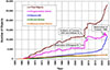 |
Figure 1 Number of objects >10 cm in LEO. Credit: NASA ODPO. |
The Iridium-Cosmos collision on 10 February 2009 at around 800 km altitude is an excellent example of an active satellite-to-debris collision in space. Before that incident, Iridium-33 was an active commercial satellite providing L-band mobile telephone and telecommunication services, while Cosmos-2251 was a defunct satellite in orbit. Besides the destruction of Iridium, the collision produced 1500–2000 pieces of potentially lethal space debris measuring ≥10 cm in diameter (Weeden, 2010). Figure 1 shows a significant increase in debris population following the Iridium-Cosmos collision and anti-satellite tests (AST) deployed for the destruction of defunct satellites in orbit (e.g., Fengyun-1C). Of the estimated pieces of debris associated with the collision, more than 29 remnants from Iridium and 60 from Cosmos have already decayed from orbit into the Earth’s atmosphere (Weeden, 2010). The destruction of Fengyun-1C also produced over 2800 cataloged fragments ≥ 5 cm (as of 2008), leading to an increase in the probability of debris collision with active satellites in specific orbits (Pardini & Anselmo, 2009). This shows that collisions pose risks not only to space assets but also to life on Earth. More recent incidents of collisions in space involved objects such as ESA’s VESPA1 and Kosmos-2143 or Kosmos-21452. The fact that all nations benefit from existing space assets makes space debris a global problem, because any satellite in orbit can be adversely affected without discrimination. Therefore, it is in the interest of all nations to collectively resolve the problem of space debris (Jakhu, 2009; SWF, 2018) and ensure a risk-free utilisation and sustainable use of the space environment (Lawrence et al., 2022).
1.2 Space weather as a player in debris generation
Space weather can adversely affect the operation of satellites in Earth orbit (e.g., Baker, 2002; Lu et al., 2019; Nwankwo et al., 2020a; Nimis et al., 2002) and consequently exacerbate the problem of debris generation in space. Adverse conditions in the space environment can damage onboard electronics and disrupt communications or navigation signals, leading to temporary service disruptions and a long-term degradation of spacecraft reliability and lifetime (SWF, 2018; Nwankwo et al., 2020b). Space weather also enhances atmospheric drag on satellites in low Earth orbit (LEO), leading to difficulties in the identification, tracking, and maneuvering of spacecrafts, as well as accelerated orbit decay (Doornbos & Klinkrad, 2006; Nwankwo et al., 2015; Nwankwo et al., 2021; Nwankwo, 2016). Atmospheric drag-induced errors in spacecraft positioning and motion can result in satellite and/or object collisions in space, especially in LEO, consequently increasing the density of space debris. Space weather-enhanced drag has also been suspected to contribute to satellite launch failures, e.g., during the SpaceX Starlink satellites launch on 3 February 2022 (Dang et al., 2022; Berger et al., 2023; Baruah et al., 2024). The 25th solar cycle is currently at its peak, and the probability of impacts from the above-mentioned associated effects (e.g., accelerated orbit decay) will increase significantly. Figure 2 depicts solar cycle effect on SATi’s orbit, where accelerated orbital decay due to enhanced atmospheric drag can be seen to be highly probable around the peak of a cycle (e.g., 2014 and 2023–2025). SATi is a hypothetical LEO spacecraft operating in a near-circular orbit at an altitude of ∼570 km in January 2014. The long-term orbital decay evolution was simulated using the proposed drag model.
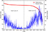 |
Figure 2 Orbital decay of SATi in relation to solar activity from January 2014 to June 2024. The red curve shows satellite altitude variation, while the blue curve represents the sunspot number (SSN). The transition between Solar cycles 24 and 25 is indicated btythe dashed vertical line. |
Some key factors for a long-term sustainable use of space include (i) the ability to monitor and understand the constantly changing space environment (achievable through improved space situational awareness) and (ii) reduction of the hazards posed by man-made orbital debris (David, 2009; Jakhu, 2009; Holzinger & Jah, 2018; SWF, 2018) This work addresses the former. The impact of the constantly changing space environment on artificial satellites, especially in the LEO, mainly arises from the interaction between the atmosphere and the spacecraft surface, leading to an aerodynamic force component termed the so-called “atmospheric or aerodynamic drag”. The ground- and space-based dynamic processes, which contribute to the heating and expansion of the upper atmosphere and consequent enhancement of drag force on LEO spacecrafts, need to be considered when modeling thermosphere density and aerodynamic drag. Such models are important for space situational awareness since they allow for proper forecast of satellites and potential debris orbit (e.g. see, Kodikara, 2019; Bruinsma et al., 2023).
1.3 Technology-driven concepts for sustainable use of the space
Beyond adherence to debris mitigation guidelines (or their enforcement), various concepts for sustainable use of the space are being actively conceived and implemented in areas such as space situational awareness (SSA), on-orbit servicing (OOS), active debris removal (ADR), and on-orbit assembly (OOA). National and international developments towards initiation and/or demonstration of these areas in past, present, and future missions include the Laser Ranging Systems Evolution Study – LARAMOTIONS (Dreyer et al., 2021), e. Deorbit (Biesbroek et al., 2017), Deutsche Orbitale Servicing Mission – DEOS (Reintsema et al., 2010), Mission Robot Vehicle MEV-1 and MEV-2 (Pyrak and Anderson, 2022), ELSA-d mission (Fujii et al., 2021), Clearspace-1 (Biesbroek et al., 2017), On-Orbit Servicing, Assembly and Manufacturing 1, OSAM-1 Coll et al. (2020). Today, the German Aerospace Center (DLR) is effectively addressing the concepts and technologies for increasing sustainability in Earth orbit within the framework of the ION (Impulsprojekt Orbitale Nachhaltigkeit) Project3. This ongoing effort combines cross-program competencies from space, security and aeronautics (especially in the areas of satellite operations, robotics and automation, space debris observation and measurement, space weather, and aerospace maintenance and repair) to pursue a holistic view of the space ecosystem, which will address short-, medium- and long-term goals in the sustainability and circular economy in orbit. The short-term goal includes the integration of relevant technology for space debris removal, life extension, and inspection into the planned orbital infrastructure. The work presented in the current paper is part of the ION project work packages that provide SSA through technologies for the (i) identification and characterization of space debris from ground and space and (ii) modeling of atmospheric drag in relation to solar activity, for the purpose of debris removal mission planning.
The modelling of atmospheric drag-induced orbital decay is generally challenging, because the proxies and contributions of individual effects of various solar (and non-solar) forcing mechanisms are not well represented in atmospheric density models (Kutiev et al., 2013; Nwankwo et al., 2015). Space weather effects, which are underrepresented in thermospheric density models (Jackson et al., 2020) can create uncertainties that widen the gap between modeled results and the actual orbital parameters. Also, because solar activity is not predictable with high accuracy, mission designers make assumptions to calculate the remaining lifetime of space probes in orbit (Fiedler & Hackel, 2012), which sometimes yields a shorter lifespan estimate, when compared to reality. However, due to these limiting factors, short-term intervals of drag on satellites in LEO can be simulated with better accuracy than long-term effects. Long-term estimation or prediction of defunct spacecraft’s orbit is even more challenging when such objects are no longer under ground control. To improve drag estimation, Wu et al. (2025) utilized historical spacecraft orbital data to derive an orbital decay factor, W, during geomagnetically quiet periods. The factor W relates variations in satellite semimajor axis to changes in thermospheric density, enabling altitude normalisation of density estimates derived from two-line element (TLE) data. This decay factor was subsequently combined with an atmospheric density proxy developed in Wu et al. (2024) to enable quasi–real-time assessment of satellite orbital decay during geomagnetic storm conditions. While this approach improved short-term drag estimation associated with geomagnetic activity, challenges in long-term drag estimation remained. Accordingly, the objective of the present work is to enhance long-term drag estimation and prediction.
In particular, we develop a robust drag model adapted to the ephemeris data-assisted calibration (EDAC) simulation method (Nwankwo et al., 2025), for improved simulation and prediction of short-term and long-term (6 months in this case) evolution of orbital decay of LEO objects as a function of solar-geophysical indices. The earlier version of this model was applied to near-circular LEO orbit to simulate space weather-enhancement of atmospheric drag and consequent orbital decay for solar minimum and maximum regimes (e.g., Nwankwo & Chakrabarti, 2014; Nwankwo et al., 2015) and the intervals of strong geomagnetic storms and associated disturbances (e.g., Nwankwo et al., 2015; Nwankwo et al., 2021; Nwankwo & Chakrabarti, 2018). Also, on a rolling basis, we leverage institutional cross-program expertise in space- and ground-based observations, modeling, and theoretical frameworks to continuously refine solar-geophysical proxies for improved atmospheric density estimation (e.g., Kodikara et al., 2021; Fernandez-Gomez et al., 2022; Forootan et al., 2022; Yuan et al., 2023; Siemes et al., 2023; Hladczuk et al., 2024). Building on these efforts, the present work focuses on improving long-term drag estimation through the application of the EDAC simulation method.
The remaining part of this paper is structured as follows: Section 2 provides the theoretical background of our drag model. Section 3 presents the data (including input solar indices and LEO objects’ orbital and ballistic parameters) and the method of analysis. The results of the analysed data and simulations are presented in Section 4, while Section 5 contains the discussion of the results. Section 6 consists of the summary and conclusion of the work.
2 Method
2.1 Atmospheric drag modeling: general theoretical considerations
The general equation of motion for a spacecraft moving under the attraction of a point mass planet with perturbation effects is given by the equation (Chobotov, 2002),
 (1)
(1)
where r is the position vector of the satellite relative to Earth’s centre, G is the Earth’s gravitational constant (G = 6.67 × 10⁻¹¹ Nm2/kg2), Me is mass of the planet (Earth in this case = 5.97 × 1024 kg) and ap is the resultant vector of all perturbing accelerations in the adverse space or near-Earth environment.
The gravitational (agf) and non-gravitational (angf) acceleration components make up the perturbing acceleration (ap). So that
 (2)
(2)
Gravitational forces include the Earth, solar and lunar attraction, and Earth’s oblateness and its triaxiality, while the nongravitational forces consist of atmospheric drag, solar radiation pressure, outgassing, and tidal effects (Wertz & Larson, 1999; Chobotov, 2002). The contribution of each force (except radiation pressure) depends on the altitude of the spacecraft (Stark et al., 2011; Curtis, 2020). In Table 1, we provide the list of major perturbing forces and their relative importance with respect to spacecrafts that are orbiting the Earth at 500 km (LEO) and Geostationary orbit (usually at ∼35,786 km) (Stark et al., 2011). The respective magnitude of perturbing accelerations (acting on the spacecraft, whose area-to-mass ratio is A/M) shows that atmospheric drag (which significantly depends on the level of solar activity) is the largest force affecting the motion of LEO satellites, as well as the only force significantly competing with the primary inverse square law gravity field of the Earth in LEO (Stark et al., 2011). At the height where the magnitude of inertial accelerations due to aerodynamic effect equals and/or exceeds the gravitational acceleration (usually at 80–100 km), the spacecraft will most likely re-enter the Earth’s atmosphere (see Fig. 3).
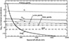 |
Figure 3 Relative magnitude of the main sources of perturbation acting upon an Earth-orbiting spacecraft (p. 105, Stark et al., 2011). |
Magnitude of perturbing accelerations acting on a space vehicle whose area-to-mass ratio is A/M (source: p. 94, Stark et al. 2011).
Another important force to reckon with in LEO is the off-center gravitational pull caused by Earth’s equatorial bulge, or oblateness. This phenomenon, commonly referred to as the J2 effect, primarily results in a secular drift of the orbital node (Ω) and perigee (ω), producing a force component directed toward the equator (Wertz & Larson, 1999; Chobotov, 2002). In this study, however, the J2 effect is neglected (as are the higher numerical expansions J3, J4, and J5 also shown in Fig. 3) because the focus is on atmospheric drag. This simplification is justified since the catalogued objects considered are located below 800 km altitude and generally spend only brief periods crossing near-equatorial regions, where the influence of J2 is comparatively less impactful. J3, J4, and J5 are zonal spherical harmonic coefficients of Earth’s gravitational potential that describe the progressive deviations of the geoid (equipotential surface of Earth’s gravity field) from a simple oblate spheroid. J3 is the dominant odd zonal harmonic and represents the north-south asymmetry of Earth’s mass distribution. It gives the geoid its characteristic “pear-shaped” form, with unequal polar radii. J3 is primarily responsible for long-period oscillations in satellite orbital elements and was first clearly detected from artificial satellite observations. J4 is an even zonal harmonic that refines the description of Earth’s oblateness beyond J2. It accounts for higher-order, equatorially symmetric flattening effects and modifies both the gravity field and the geoid shape while preserving hemispheric symmetry. J5 is an odd zonal harmonic of smaller magnitude. Like J3, it contributes to hemispheric asymmetry, but its effect is weaker and represents finer-scale distortions of the geoid. Its influence is mainly seen in subtle periodic satellite perturbations rather than large geometric effects (Von Puttkamer, 1969).
The drag or negative acceleration, adrag experienced by the spacecraft is given as (Bate et al., 1971; Wertz & Larson, 1999; Chobotov, 2002):
 (3)
(3)
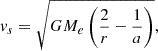
where ρ is the altitude-dependent atmospheric density. ρ is obtained from the NRLMSISE-00 model described in Section 3.2. Cd is the unitless atmospheric drag coefficient (Moe et al., 1995, 1998; Moe & Moe, 2005), As is the spacecraft’s projected area in the direction of motion, ms is the mass of the spacecraft and vs is the relative spacecraft velocity with respect to the environment or neutral winds. As, Cd and ms are related through the spacecraft’s ballistic coefficient B and expressed as (Wertz & Larson, 1999; Chobotov, 2002):
 (4)
(4)
The velocity of a spacecraft in circular orbit is expressed as (Chobotov, 2002):
 (5)
(5)
The velocity of a spacecraft in an elliptical orbit (depicted in Fig. 4) is given by the equation (Chobotov, 2002):
 (6)
(6)
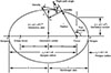 |
Figure 4 Geometry for spacecrafts in elliptical Earth’s orbit (Chobotov, 2002, p. 26). |
where a is the semimajor axis.
Atmospheric drag force is strongest at the perigee of a spacecraft in an elliptical orbit. When under the influence of the negative impulse of drag at the perigee, the elliptical orbit becomes more circular in each revolution, until the apogee altitude reduces to the value of the perigee (Chobotov, 2002; Colombo & McInnes, 2010; Huang et al., 2022). When this happens, r ≈ a, so that equation (6) reduces to equation (5).
The radius r (satellite’s position) is generally represented by (Bate et al., 1971; Chobotov, 2002):
 (7)
(7)
where P is the semilatus rectum, e is the eccentricity of the orbit and f is the true anomaly. The parameters a, P and e can be expressed as (Chobotov, 2002):
 (8)
(8)
where ra is the radius (or height) of the apogee and rp the radius of the perigee expressed as ra = a(1 + e) and rp = a(1 - e), respectively.
 (9)and
 (10)
(10)
The true anomaly (f) can be calculated using the equation (Chobotov, 2002):
![Mathematical equation: $$ f=2\mathrm{arctan}\left[{\left(\frac{1+e}{1-e}\right)}^{\frac{1}{2}}\mathrm{tan}\frac{E}{2}\right]. $$](/articles/swsc/full_html/2026/01/swsc250083/swsc250083-eq44.gif) (11)
(11)
where E is the eccentric anomaly expressed as E ≈M + e sin M (if the mean anomaly (M) is known). The true anomaly (f) can be defined as the angle at the focus F between the direction of perihelion (or perigee) and the radius r of the body (as demonstrated in Fig. 4).
The decay rate of the satellite’s semimajor axis a is theoretically given by (Chobotov, 2002):
 (12)
(12)
 represents the mean motion (n) of the spacecraft (Chobotov, 2002; Doornbos, 2012).
The latitude (L) of the spacecraft (i.e., latitude of the point directly beneath the satellite on Earth) and its longitude (φ) on the celestial sphere are governed by the equations (4) and (6) of Washburn (2004).
 (13)
(13)
 (14)
(14)
L and φ are determined by the inclination of the orbit (i) and f (defined above). The satellite’s location is a periodic function of both f and time.
The formulation of the drag model is based on the above theoretical framework. We used the numerical integration method4 in the spherical coordinate system for the orbit propagation. The dynamical system evolves the radial distance (r), radial velocity (vr), angular position (ϕ) and angular rate ( ) as coupled differential equations under Earth’s gravity and atmospheric drag (Nwankwo et al., 2021).
 (15)
(15)
 (16)
(16)
 (17)
(17)
 (18)
(18)
 and
and  are the radial and tangential acceleration components. The basic equations (e.g., (5)–(11)) are introduced into the coupled equations via r and
  (
( ).
).
2.2 Long-term drag estimates using ephemeris data-assisted calibration simulation
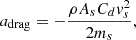
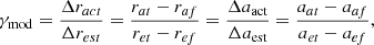
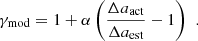
In this section, we introduce an object-specific Drag Normalization Coefficient (DNC), denoted γmod, derived using the EDAC method (as illustrated in Fig. 5) to improve long-term orbital decay prediction of LEO objects. The DNC acts as a unitless scaling factor applied to the drag-induced rate of change of the spacecraft semimajor axis, compensating for aggregate uncertainties in drag modeling arising from time-varying ballistic coefficients, unresolved attitude dynamics, atmospheric density biases, and unmodeled perturbations. The proposed approach preserves physical transparency in the drag-orbit coupling (without modifying underlying physical models) while correcting the net bias accumulated over long propagation horizons. The DNC is estimated by comparing observed semimajor-axis decay extracted from historical ephemeris data with decay predicted by a nominal drag model over a selected calibration interval. When incorporated into forward propagation, the modulated drag model reproduces long-duration orbital decay trajectories that closely match historical decay records of LEO objects, enabling realistic and computationally efficient long-term decay prediction without reliance on detailed object-specific drag characterisation. We thus express the γmod as:
 (19)
(19)
 |
Figure 5 The concept of ephemeris data-assisted calibration (EDAC) method for improving long-term drag simulation. (a) unmodulated simulation of a LEO spacecraft’s mean height (r) and (b) EDAC normalised simulation of r. |
where  or
or  is the difference between the actual spacecraft positions at time t, r at, and some future time f, r af and Δr est or Δa est is the difference between the estimated positions r et (r ef) at the times t(f). Note that γmod is a unitless normalisation factor, adjusted to be close to 1. The time difference between t and f (Δt) can be an orbital period or several orbits. However, the application of a DNC is recommended when the model’s integrated decay bias exceeds the practical drag-uncertainty envelope – typically on the order of 10–20% in Δaact over the calibration arc, or equivalently when
  . Such behavior indicates that unmodeled object-specific drag effects and/or atmospheric density biases dominate the long-term prediction error.
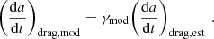
As an alternative to enforcing an exact match of the cumulative decay over the calibration arc, a regularized form of the DNC may be employed to mitigate overfitting to short-duration ephemeris data. In this formulation, the modulation factor is expressed as:
 (20)
(20)
where α ∈ (0,1] controls the strength of the correction. This expression interpolates between the unmodified drag model (α = 0) and the fully calibrated single-arc EDAC solution (α = 1), allowing partial correction of the net semimajor axis decay bias while preserving model robustness in the presence of the model-associated uncertainties.
The DNC is then applied as a multiplicative correction to the drag-induced rate of change of the spacecraft semimajor axis, such that
 (21)
(21)
2.3 Estimation of short-term drag enhancement by geomagnetic storm
Several flares and geomagnetic storms were recorded during Jan–Jun 2024, with more than 8 storms having Kp > 6 (or Ap > 100), including the extreme storm of 10–11 May (Hayakawa et al., 2025). However, to assess the impact of geomagnetic storms on atmospheric drag, we investigate only the extreme geomagnetic storm of 10–11 May 2024. The unique characteristics of each storm case depend on their respective interplanetary drivers – e.g., coronal mass ejection (CME) or corotating interactive region (CIR) and/or high solar wind streams (HSS). The CME-driven storm has a stronger magnetospheric convection electric field strength than a CIR/HSS-driven storm (Denton et al., 2006), while a CIR/HSS-driven storm and associated effects propagate longer than a CME-storm (Chen et al., 2012). However, because the consideration of these drivers and associated dynamics is beyond the scope of the present work, the authors refer readers to related articles such as Knipp et al. 2004, Prölss, 2011. In general, the energy input into the Ionosphere-Thermosphere (IT) system during storms significantly increases, and results in joule heating. Particle precipitation (electrons and protons) can also play a role on smaller scales5. Storms drive short-term but strong heating of the upper thermosphere, which can lead to severe perturbation of the orbital motion of spacecraft. The daily orbit decay rate (ODR D) and ODR associated with the storm day (ODR S) can be estimated using the expressions:
![Mathematical equation: $$ \mathrm{OD}{\mathrm{R}}_D=\sum_{i=1}^{{N}_{\mathrm{day}}} \left[{a}_i-{a}_{(i-1)}\right], $$](/articles/swsc/full_html/2026/01/swsc250083/swsc250083-eq94.gif) (22)
(22)
 (23)
(23)
ODRM is the mean ODR for the month. The above expression can also be referred to as the specific storm-induced ODR (SSIO). Storms sometimes have overlapping effects on the day (or days) before and/or after the main phase of the events, depending on their driver, initiation, commencement, and/or duration (Knipp et al., 2005; Olabode & Ariyibi, 2020). Considering a number of storm active days (N), the total orbit decay (TODS) associated with the storm can thus be calculated from:
 (24)
(24)
3 Data
3.1 Space object parameters
A debris removal mission usually consisst of robotic and satellite technologies for rendezvous, proximity operations, and subsequent capture of space debris objects or target (Ledkov & Aslanov, 2022; Borelli et al, 2023). We will thus provide a model-based space and orbital situational awareness of selected targets through the analysis of space weather influence on the objects’ trajectory for the period of January to June 2024. The list of selected cataloged LEO objects and their orbital and ballistic parameters is provided in Table 2. The 8 objects were selected based on their height (at the start of this investigation) and possession of retro reflectors for enhanced observability from ground-based facilities. Typically, the height of the objects ranges from ≃512 to 689 km. However, for convenience, we categorised the objects into 2 height-dependent groups – Group A at 500 < h < 600 km and Group B at 600 < h < 700 km. Figure 6 shows the distribution of objects within the respective groups and the separation between them. Group A objects are distributed within a 53 km range, while those in group B are distributed within a 64 km. The separation between the last group A object (ASAP-S) and the first group B object (HELIOS-1B) is ∼60 km.
 |
Figure 6 Representation of height-dependent grouping, distribution, and separation of the investigated LEO objects. Group A objects are distributed within a 53 km range, group B are distributed within a 64 km and the separation between the last group A object (ASA) and the first group B object (HEL) is ∼60 km. Each diamond represents an object listed accordingly in Table 2. |
The orbital and ballistic parameters of selected objects.
The historical orbital data, such as the mean height (h), eccentricity (e), and inclination (i) of the objects were obtained from a comprehensive satellite catalog6. Their mass (ms), projected cross-sectional area (As), and shape were obtained from ESA’s DISCOSweb7. e can also be calculated from equation (10). The drag coefficients (Cd) were assumed based on the shape-dependent recommendations in Moe et al. (1995, 1998) and Moe & Moe (2005). Table 3 provides information on the shape of the objects. In this work, the specific orbital and ballistic parameters of each object will be used to simulate their peculiar orbital trajectory and associated solar activity-modulated environment. The daily solar radio flux (F10.7) and geomagnetic Ap during the period of investigation (Jan–June 2024) are shown in Figure 7.
 |
Figure 7 Observed daily solar radio flux (F10.7) in solar flux unit (sfu = 10-22 Wm-2 Hz-1) and geomagnetic Ap during Jan–June 202410. |
The objects’ shape, maximum, minimum, and mean As (source: ESA’s DISCOSWeb).
3.2 Thermospheric density (ρ) estimates
The altitude-dependent thermospheric density, ρ, is obtained from the NRLMSISE-00 empirical atmospheric model (Picone et al., 2002), which consists of parametric and analytic approximations to physical theory for the vertical structure of the atmosphere as a function of time, location, and solar and geomagnetic activity. The main input related to solar-geophysical indices was the daily F10.7 and 3-h Ap index (shown in Fig. 7). These indices are used to parameterise solar and geomagnetic forcings (see, e.g., Gaposchkin and Coster, 1988; Picone et al., 2002; Doornbos, 2012).
4 Results
4.1 Analysis of long-term effects of space weather on the objects’ aerodynamic drag
Figure 8 shows the actual mean height (h-ACT) obtained from the historical orbital data and the simulated mean heights (h-SIM) of group A objects (ELSA-D, GFO-1, OICETS, and ASAP-S) and their corresponding orbit decay rates (ODR-ACT, ODR-SIM), modeled as a function of the observed solar-geophysical indices during January to June 2024. The respective h-ACT and h-SIM of the objects on 1 January and 30 June, and the γmod normalisation factor used to achieve the simulated long-term decay scenario is provided in Table 4. Based on this detail, their actual total orbital decay (TOD-ACT) is ∼34.4, 12.7, 16.5, and 8.5 km, respectively, while the simulated total decay (TOD-SIM) is ∼35.9, 13.1, 17.0, and 8.7 km, respectively. The objects TOD-SIM were generally higher than TOD-ACT by ∼1.5, 0.7, 0.5, and 0.2 km, respectively. These values correspond to a respective percentage error (δ) of about 4.3, 3.2, 2.8, and 2.1%. The obtained results are for objects that are orbiting Earth at a typical altitude range of ∼512–565 km, and the combined mean TOD-ACT and TOD-SIM for this height range are 18.04 and 18.68 km, respectively.
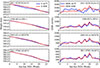 |
Figure 8 The actual mean height (h-ACT) and simulated mean height (h-SIM) of ELSA-D, GFO-1, OICETS, and ASAP-S as a function of the observed solar-geophysical indices during Jan–Jun 2024 and their corresponding orbit decay rates (ODR-ACT, ODR-SIM). |
Analysis of the actual and simulated mean heights (h-ACT, h-SIM) of ELSA-D, GFO-1, OICETS, and ASAP-S for 01.01.2024 – 30.06.2024 (DD.MM.YYYY) and their respective γmod normalisation factor.
Figure 9 shows the h-ACT and h-SIM of HELIOS-1B, RESURS-1, SOHLA-1, and GALEX and their corresponding orbit decay rates (ODR-ACT, ODR-SIM) as a function of the observed solar-geophysical indices during Jan to June 2024. These objects fall within the Group B category, with the typical height range of ∼625–689 km. Their respective h-ACT and h-SIM on 1 January and 30 June, and the γmod normalisation factor used to achieve the simulated long-term decay for the interval is provided in Table 5. The TOD-ACT values for the objects during the interval are ∼2.56, 3.13, 1.73, and 0.15 km, respectively, while the corresponding TOD-SIM values are ∼2.65, 3.24, 1.84, and 1.60 km. Similar to the previously analysed cases, the objects’ TOD-SIM are slightly higher than TOD-ACT by ∼0.1, 0.1, 0.1, and 0.2 km, respectively, which corresponds to a respective δ of about 3.4, 3.5, 6.0, and 7.5%. For this altitude range, the combined mean values of TOD-ACT and TOD-SIM are 2.2 km and 2.3 km, respectively. These results indicate that Group A objects experienced an approximately eightfold stronger drag impact than Group B objects, despite an altitude separation of only 60 km.
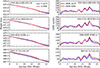 |
Figure 9 The actual mean height (h-ACT) and simulated mean height (h-SIM) of HELIOS-1B, RESURS-1, SOHLA-1, and GALEX as a function of the observed solar-geophysical indices during Jan–Jun 2024 and their corresponding orbit decay rates (ODR-ACT, ODR-SIM). |
Analysis of the actual and simulated mean heights (h-ACT, h-SIM) of HELIOS-1B, RESURS-1, SOHLA-1, and GALEX and associated γmod during 01.01.2024 to 30.06.2024 (DD.MM.YYYY).
4.2 Analysis of short-term aerodynamic drag enhancement due to geomagnetic storm
In this section, we estimate the 4 days (10–13 May) accumulated impact of the reference storm on the objects using the simulated results. In Figure 10, we show the observed daily mean values of F10.7 and Ap and the simulated ODR of the objects for 8–14 May 2024. The approximate height of the objects at the time of impact, the pre-storm day ODR (ODR PS), the mean daily ODR on 10–13 May (ODRD10-D13) and the estimated mean atmospheric density (ρ) during the storm main phase on 11 May 2024 are provided in Table 6. Similarly, their respective TOD for the month, the mean ODR for the month ( ), the storm-induced ODR for each day during 10–13 May (ODRS10-S13) and the 4-day [combined] storm-induced total TODS are provided in Table 7. ODRD10-D13 were excluded from the computation of
  to prevent contamination of the quiet-time background. ODRS10-S13 and TODS were estimated based on equations (23) and (24), respectively. The results show a height-dependent drag effect with the maximum impact occurring on 11 May 2024. However, there are a few exceptions to the impact dependency on the objects’ height, which we believe are coupled to their individual ballistic coefficients. Relative to the pre-storm mean reference values (ODR PS; Table 6), the orbital decay rates increased by 248.5%, 232.8%, 245.6%, 241.3%, 256.7%, 264.7%, 266.0% and 259.4% for the respective objects. When referenced to the monthly mean values (ODRM; Table 7), the corresponding increases were 213%, 217%, 234%, 229%, 233%, 239%, 243% and 236%. Because ODRPS and
  are comparable, the resulting storm-time ODR enhancements derived using either reference are consistent, differing only modestly while preserving both their magnitudes and relative ordering across spacecraft.
 |
Figure 10 The observed daily F10.7 and Ap and the simulated objects’ orbit decay rate (ODRD) for 8–14 May 2024. The black and red bars represent F10.7 and Ap indices, respectively. The blue bar represents the ODR, and the orange line indicates the monthly mean ODR (baseline). The left panel is for Group A objects and the right panel for Group B objects. |
Mean daily ODR (ODRD) during 10–13 May 2024 and mean ρ on 11 May.
Analysis of specific storm-induced ODR (SSIO) for 10–13 May 2024.
To further demonstrate the observed dependency of the storm (and atmospheric drag) impact level on the objects’ height, we show in Figure 11 the ODR D of objects in group A and group B during 1–30 May 2024. Their ballistic coefficients (B) and approximate heights at the time of impact are also indicated. Considering their typical height range and separation (as described in Sect. 3.1 using Fig. 6), the combined mean ODR of group A on 10th, 11th, 12th, and 13th DOM were 148 m/day (ODR S10), 165 m/day (ODR S11), 63 m/day (ODR S12) and 31 m/day (ODR S13), respectively, which corresponds to a TOD S of 407 m, while the respective ODRS(10–13) of group B are 23, 24, 9, and 5 m/day, corresponding to TOD S of 61 m. Given the ∼60 km separation between the two altitude groups, the geomagnetic storm produced an approximately sevenfold larger increase in ODR for objects at 500 < h < 600 km than for those at 600 < h < 700 km. To quantify the storm-driven variability in thermospheric density at the respective group altitudes and its contribution to the observed impact levels, Table 6 reports the mean atmospheric density evaluated at the object altitudes. The mean combined thermospheric density at Group A altitude, ρgroup-A, is 2.72 × 10 -12 kg/m3, whereas the corresponding value at Group B altitude, ρgroup-B, is 6.77 × 10 -13 kg/m 3. On average, Group A experiences approximately four times the atmospheric density of Group B (ρgroup-A/ρgroup-B ≈ 4.0). Despite this fourfold density difference, the mean orbital decay rate in Group A is nearly seven times larger, indicating that the storm-time response is influenced by the combined effects of atmospheric density, object-specific ballistic properties, and orbital dynamics rather than density alone.
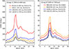 |
Figure 11 The ODR for objects in Group A (500 < h < 600 km) and Group B (600 < h < 700) during 1–30 May 2024. |
In addition to object altitude, as demonstrated by the results, object-specific orbital and ballistic parameters play a critical role in determining aerodynamic drag severity. The ballistic coefficient, B, of the objects selected for this work ranges between 0.0058 and 0.0278 m 2/kg (see Table 2). Figure 12 shows the objects’ B and total orbit decay (TOD S) against their altitudes at the time (and duration) of storm impact. The results show enhanced orbital decay (via TOD S) for objects that have larger B at higher altitude (e.g., OICETS, RESURS) than relatively lower height objects with smaller B (e.g., GFO-1, HELIOS). The TOD S of OICETS at ∼543 km is ∼397 m, while GFO-1 is ∼280 m at ∼531 km. Similarly, the TOD S of RESURS (at ∼631 km) is ∼84 m/day, while that of HELIOS (∼623 km) is ∼65 m.
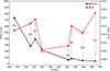 |
Figure 12 The object’s ballistic coefficient (B) and storm-associated total orbit decay (TODS) against their altitudes at the time and duration of storm impact (10–13 May 2024). |
5 Discussion
The investigated objects vary considerably in shape, orbital, and ballistic parameters (see Tables 2 and 3), yet the EDAC simulated results in the long-term regime compared well with their historical orbital data. The percentage error of the simulated total orbital decay (TOD-SIM) of the objects was less than 10%. In general, the trend in variation of the objects’ TOD shows strong dependency on the height and ballistic coefficient (B). Objects at altitudes of 500–565 km experienced approximately eight times stronger aerodynamic drag than those at 600–689 km. This difference is partly attributable to the exponential decrease in thermospheric density with altitude, whereby higher ambient density leads to increased drag forces and accelerated orbital decay (Doornbos et al., 2013; Nwankwo and Chakrabarti, 2014; Zesta and Huang, 2016; Nwankwo et al., 2021), as demonstrated by the height-dependent density variations reported in Table 6. The influence of B on drag is demonstrated in the decay scenario between GFO-1 (at ∼539 km) and OICETS (∼553 km) and between HELIOS (∼625 km) and RESURS (∼633 km). OICETS (with B = 0.024 m2 kg−1) experienced more drag (or decay) than GFO-1 (B = 0.021 m2 kg−1) despite being at a higher altitude (where the drag effect is relatively less) due to its larger B. B accounts for the shape and mass of the objects and is connected to the spacecraft’s projected area (As) and Cd through equation (4). As can change when the object’s attitude (or orientation) changes and the Cd can also change due to external temperature, spacecraft’s material, and the angle with which particles are deflected off by the satellite’s surface (Moe & Moe, 2005; McLaughlin et al., 2011; Bernstein & Pilinski, 2022). These factors can influence B. Assuming the same mass ms (and Cd) for two objects, and differences in As, the one with the larger As will experience greater drag force and a consequent increase in orbit decay rate than those with smaller As (Chobotov, 2002; Nwankwo &Chakrabarti, 2015; Nwankwo et al., 2021). Also, spacecraft with a high B (such as OICETS) typically have low mass and a large surface area relative to their volume, making them highly susceptible to the low-density upper atmosphere and its variations caused by solar activity (e.g., Miyata et al., 2018; Marianowski et al., 2025). Therefore, the difference in the respective As for OICETS and RESURS (associated with shape), is a major contributor to the increase in their ODR.
It is worth noting that there is a striking agreement in the signature of the long-term evolution of the objects’ orbital decay for both the actual and simulated scenarios (see Figs. 8 and 9). This signature is connected to solar cycle variability as demonstrated in Figure 13, where the long-term evolution of the objects’ ODR was compared with solar-geophysical indices of the corresponding interval. The thermospheric density varies with solar and geomagnetic activity, which causes thermospheric heating and expansion of the thermosphere and also reflects solar cycle variation (Knipp et al., 2005). Consequently, atmospheric drag-induced orbital decay and the lifetime of spacecrafts reflect solar cycle variation in density (Walterscheid, 1989). The solar cycle-induced feature or signature observed in the orbit decay rate (ODR-ACT, ODR-SIM) of the objects appears to be lacking in ELSA-D’s ODR evolution (see Fig. 8, top panel). To investigate this seeming anomaly, we obtained and shown in Figure 14 the orbital history of ELSA-D during Jan 2023 to April 2024. The historical orbital data show a trajectory pattern that appears to be related to the object’s operational characteristics. Figure 13 also showed the corresponding spike in the ODR during the intervals of accelerated orbital decay. The ELSA-D spacecraft was designed to simulate and validate the technologies for end-of-life spacecraft retrieval and disposal services8. Consequently, it demonstrated capabilities that are essential for on-orbit servicing, such as rendezvous maneuvers and captures and proximity operations during its active mission phase9. An anomalous spacecraft condition was also detected in ELSA-D during the period of its technology demonstration (see Footnote 9). We therefore conclude that the comparatively weak solar-activity signature observed in ELSA-D’s ODR, relative to the other objects, may be attributable to its operational characteristics. Our model assumed a trajectory evolution that is consistent with the surrounding space environment. We also note the relatively sharp drop in the objects’ height and the consequent large increase in their ODR (in Figs. 8 and 9), which started within week 18. This effect is associated with the severe geomagnetic storm, which lasted for several days starting on 10 May 2024.
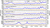 |
Figure. 13 Seven-day mean ODR of ELSA-D, GFO-1, OICETS, RESURS-O1 and SOHLA-1 compared with Ap and F10.7 indices during January 2023 to June 2024. |
 |
Figure. 14 Orbital history of ELSA-D during Jan 2023 to April 2024. |
The geomagnetic storm of 10–11 May 2024 was associated with significant elevation of solargeophysical indices (Kp of up to 9 or Ap ~ 400 and F10.7 ~ 223). The elevated solar-geophysical indices implied a strong thermospheric heating by solar EUV (represented via F10.7 proxy), plus additional Joule heating from geomagnetic perturbations (via Ap proxy). The storm driven short-term intense heating of the magnetosphere-ionosphere-thermosphere system can expand the upper thermosphere and lead to enhanced atmospheric drag on LEO objects (Mandea et al., 2019; Nwankwo et al., 2021). Similar to the analysed long-term decay evolution, the drag force exerted on the object during the severe storm was significantly influenced by the B and height of the object, which is strongly reflected in the obtained results published here (see, Figs. 11 and 12 and Table 6). Other factors that can influence drag impact include the object’s operational dynamics and coordinates. When a spacecraft’s mounting location is oriented towards the sun on the dayside, atmospheric drag force (which is proportional to the increased atmospheric density on the dayside and the spacecraft’s As facing the direction of motion) will increase, leading to a greater rate of orbital decay (e.g., Colombo & McInnes, 2010). Although the storm-induced increase in the objects ODR varied between 233% and 266% on 11th DOM (relative to pre-storm value), the mean daily ODR percentage increase (of ELSA-D) is -249%. This is in good agreement with Wu et al. (2025), who reported observed (and estimated) daily ODR increase of about 560 (and 580) m/day on 11 May 2024 for FY-3G spacecraft with B −0.015 m2/kg (based on ballistic parameters obtained from DISCOSweb) at the mean height of −414 km. The decay rate compares well with simulated ODR of 549 m/day for ELSA-D (B = 0.017 m2 kg−1) at a higher altitude of −492 km. Other objects investigated in the present work are well above the height of FY-3G.
The γmod normalisation factor proved important for achieving a good estimate of long-term drag effect. It is generally lower for strong drag (or solar active) scenario and tend to depend on the object’s altitude and ballistic (and orbital) parameters. To provide an insight into how the γmod is connected to the orbital and ballistic parameters of the objects, we show in Figure 15 the Pearson correlation coefficients of γmod dependency of the objects height, ballistic coefficient and inclination. γmod appear to have a good anti-correlation with the heights of the objects (r = −0.64). For the present investigation it tends to decrease with increasing height. It also has strong anti-correlation with B (r = −0.79). Objects with large B are highly susceptible to atmospheric drag force, especially when their A/M ratio is high (White et al., 2013; Miyata et al., 2018). GFO, OICETS, RESURS and GALEX have large B but their γmod is smaller when compared to objects with smaller B value. GALEX has the largest B with the lowest γmod and RESURS is at a relatively higher orbit (−630 km), yet its γmod is comparable to that of GFO in lower orbit. We also see a good correlation between γmod and the objects inclination (r = 0.61). However, the apparent dependence of γmod on inclination is not robust because the result appears to be largely influenced by GALEX rather than reflecting a systematic inclination effect across the debris population – indicating that inclination may not be an independent driver of drag normalisation. Therefore, a more accomplished investigation of γmod normalisation factor is required for a better interpretation of its dependence on spacecrafts orbital and ballistic parameter. Such investigation should include the analysis of multi-spacecraft dynamic parameters, the constantly varying space environment and possible influence of other perturbing forces (e.g., solar radiation pressure (SRP)), which are beyond the scope of this work. Although we assumed (in the present analysis) that SRP is negligible at the objects’ typical height range of 512–689 km (Alessi et al., 2018), it will be worthwhile to investigate their significance, especially at h > 600 km. Other factors that can influence the simulated result include the estimated or constant Cd, As and possible errors in atmospheric density models (Picone et al., 2002; Wang et al., 2024).
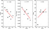 |
Figure. 15 Pearson correlation coefficients of γmod dependency of the objects altitude, mean height (h), ballistic coefficient (B) and inclination (i). |
6 Summary and conclusion
This study applied the ephemeris data-assisted calibration (EDAC) method to simulate the long-term orbital decay of 8 catalogued LEO objects driven by space weather-enhanced atmospheric drag during the period January–June 2024. The analysis incorporated observed solar-geophysical indices and classified the objects into two altitude groups spanning 500–600 km and 600–700 km. In general, the EDAC-based simulations showed good agreement with historical orbital data, with only modest altitude-dependent deviations. Objects operating at lower altitudes (~512–565 km) experienced drag impacts up to 8 times stronger than those at higher altitudes (624–689 km), consistent with the exponential decrease of thermospheric density with altitude. We also investigated short-term drag enhancements associated with the severe geomagnetic storm of 10–11 May 2024, and the results revealed storm-time increases in orbital decay rates of about 233–266% during the main phase. For a vertical separation of ~60 km, storm-related drag impacts differed by a factor of 7 between the two altitude groups. The analysis further demonstrates that storm-time and long-term drag responses vary substantially from object to object, reflecting the combined influence of altitude-dependent atmospheric density, object-specific orbital dynamics, ballistic properties, and operational characteristics. Both the EDAC simulations and historical orbital data consistently captured the signatures of solar activity over the investigated period, reinforcing the consistency of the proposed modeling framework. Overall, the results indicate that the EDAC approach provides improved fidelity in long-term orbital decay and drag modeling and represents a valuable tool for both predictive and diagnostic assessment of drag impacts in LEO. We note, however, that the present simulations utilised mean projected areas for the objects, whereas most operational spacecraft typically experience varying cross-sectional area in flight. While the agreement with historical orbital data supports the suitability of the approach for long-term drag estimation, future work will incorporate adaptive drag normalisation, rather than a single global DNC, to more accurately capture regime-dependent drag behaviour as objects traverse varying thermospheric density conditions. These results have direct implications for SSA, mission planning and operations, as improved long-term drag characterisation enhances orbit prediction accuracy, conjunction assessment reliability, and re-entry forecasting for LEO objects under both quiet and disturbed space weather conditions.
Acknowledgments
The authors thank the reviewers for their constructive and valuable comments, which significantly improved the quality of this manuscript. The editor thanks William Denig and Sumanjit Chakraborty for their assistance in evaluating this paper.
Funding
This work was supported by the research project “Impuls Orbitale Nachhaltigkeit” (ION) of the German Aerospace Center (DLR).
Conflicts of interest
The authors declare no conflicts of interest.
Data availability statement
The objects’ mass, effective projected area, and shape were obtained from ESA DISCOSWeb (https://discosweb.esoc.esa.int/). Their historical orbital data were obtained from In-the-sky.org satellite catalog (https://in-the-sky.org/). The objects historical mean heights were extracted using WebPlotDigitizer (https://automeris.io/). The Ap index and the F10.7 radio flux observations were obtained from the database GFZ Helmholtz Centre for Geosciences, Germany (https://kp.gfz.de/en/data).
Supplementary material
Supplementary File 1: Secure World Foundation. 2018. Space sustainability: A practical guide. Updated 2018. Secure World Foundation, Broomfield, CO. Access Supplementary Material
References
- Alessi, EM, Schettino G, Rossi A, Valsecchi GB. 2018. Solar radiation pressure resonances in Low Earth Orbits, Mon Not R Astron Soc 473 (2): 2407–2414. https://doi.org/10.1093/mnras/stx2507. [Google Scholar]
- Baker, DN. 2002. The occurrence of operational anomalies in spacecraft and their relationship to space weather. IEEE Trans Plasma Sci 28 (6): 2007–2016. https://doi.org/10.1109/27.902228. [Google Scholar]
- Baruah, Y, Roy S, Sinha S, Palmerio E, Pal S, et al. 2024. The loss of the Starlink satellites in February 2022: How moderate geomagnetic storms can adversely affect assets in Low-Earth orbit. Space Weather 22 (4): e2023SW003716. https://doi.org/10.1029/2023SW003716. [Google Scholar]
- Bate, RR, Mueller DD, White JE. 1971. Fundamentals of astrodynamics. Courier Dover Publications, New York. https://cmp.felk.cvut.cz/~kukelova/pajdla/Bate,%20Mueller,%20and%20White%20-%20Fundamentals%20of%20Astrodynamics.pdf. [Google Scholar]
- Berger, TE, Dominique M, Lucas G, Pilinski M, Ray V, et al. 2023. The thermosphere is a drag: The 2022 Starlink incident and the threat of geomagnetic storms to low earth orbit space operations. Space Weather 21, e2022SW003330. https://doi.org/10.1029/2022SW003330. [CrossRef] [Google Scholar]
- Bernstein, V, Pilinski M. 2022. Drag coefficient constraints for space weather observations in the upper thermosphere. Space Weather, 20: e2021SW002977. https://doi.org/10.1029/2021SW002977. [CrossRef] [Google Scholar]
- Biesbroek, R, Innocenti L, Wolahan A, Serrano SM. 2017. e. Deorbit-ESA’s active debris removal mission. In: Proceedings of the 7th European Conference on Space Debris (Vol. 10), April, ESA Space Debris Office. https://conference.sdo.esoc.esa.int/proceedings/sdc7/paper/1053/SDC7-paper1053.pdf. [Google Scholar]
- Biesbroek, R, Aziz S, Wolahan A, Cipolla SF, Richard-Noca M,et al. 2021. The clearspace-1 mission: ESA and clearspace team up to remove debris. In: Proc. 8th Eur. Conf. Sp. Debris, April, pp. 1–3. https://conference.sdo.esoc.esa.int/proceedings/sdc8/paper/320/SDC8-paper320.pdf. [Google Scholar]
- Borelli, G, Gaias G, Colombo C. 2023. Rendezvous and proximity operations design of an active debris removal service to a large constellation fleet. Acta Astronautica , 205: 33–46. 10.1016/j.actaastro.2023.01.021. [Google Scholar]
- Bruinsma, S, Dudok de Wit T, Fuller-Rowell T, Garcia-Sage K, Mehta P, et al. 2023. Thermosphere and satellite drag. Adv Space Res. https://doi.org/10.1016/j.asr.2023.05.011. [Google Scholar]
- Chen, GM, Xu J, Wang W, Lei J, Burns AG. 2012. A comparison of the effects of CIR-and CME-induced geomagnetic activity on thermospheric densities and spacecraft orbits: Case studies. J Geophys Res Space Physics 117 (A8): A08315. https://doi.org/10.1029/2012JA017782. [Google Scholar]
- Chobotov, VA. 2002. Orbital mechanics. AIAA. https://doi.org/10.2514/4.862250. [Google Scholar]
- Coll, GT, Webster GK, Pankiewicz OK, Schlee KL, Aranyos TJ, et al. 2020. NASA’s Exploration and In-Space Services (NExIS) Division OSAM-1 Propellant Transfer Subsystem Progress 2020. In: 2020 AIAA Propulsion and Energy Forum, August. https://ntrs.nasa.gov/citations/20205004116. [Google Scholar]
- Colombo, C, McInnes C. 2010. Orbital dynamics of earth-orbiting’ smart dust’ spacecraft under the effects of solar radiation pressure and aerodynamic drag. In: AIAA/AAS Astrodynamics Specialist Conference, 7656. https://doi.org/10.2514/6.2010-7656. [Google Scholar]
- Curtis, HD. 2020. Orbital mechanics for engineering students: Revised Reprint. Butterworth-Heinemann. https://shop.elsevier.com/books/orbital-mechanics-for-engineering-students/curtis/978-0-12-824025-0. [Google Scholar]
- Dang, T, Li X, Luo B, Li R, Zhang B, et al. 2022. Unveiling the space weather during the Starlink satellites destruction event on 4 February 2022. Space Weather 20, e2022SW003152. https://doi.org/10.1029/2022SW003152. [CrossRef] [Google Scholar]
- David, L. 2009. Orbital debris cleanup takes center stage. SPACE.com. 7 October 2009. Available at: https://www.space.com/7377-orbital-debris-cleanup-takes-center-stage.html (Accessed: 10 Sept. 2023). [Google Scholar]
- Denton, MH, Borovsky JE, Skoug, MF Thomsen, Lavraud B, et al. 2006. Geomagnetic storms driven by ICME-and CIR-dominated solar wind. J Geophys Res Space Physics 111, A7. https://doi.org/10.1029/2012JA017782. [Google Scholar]
- Doornbos, E, Bruinsma S, Pilinski MD, Bowman B. 2013. The need for a standard for satellite drag computation to improve consistency between thermosphere density models and data sets. In: 6th European Conference on Space Debris, 723, p. 71. https://conference.sdo.esoc.esa.int/proceedings/sdc6/paper/130/SDC6-paper130.pdf. [Google Scholar]
- Doornbos, E. 2012. Thermospheric density and wind determination from satellite dynamics. In: Theses, Springer, Berlin Heidelberg. https://doi.org/10.1007/978-3-642-25129-0. [Google Scholar]
- Doornbos, E, Klinkrad H. 2006. Modelling of space weather effects on satellite drag. Adv Space Res 37 (6): 1229–1239. https://doi.org/10.1016/j.asr.2005.04.097. [Google Scholar]
- Dreyer, H, Scharring S, Rodmann J, Riede W, Bamann C, et al. 2021. Future improvements in conjunction assessment and collision avoidance using a combined laser tracking/nudging network. In: Proceedings of the 8th European Conference on Space Debris, virtual conference, 20–23 April 2021, Paper 153, ESA Space Debris Office, Darmstadt, Germany. https://elib.dlr.de/142042/. [Google Scholar]
- ENISA. 2025. Space threat landscape. Report 2025. European Union Agency for Cybersecurity (ENISA). https://www.enisa.europa.eu/sites/default/files/2025-03/Space_Threat_Landscape_Report_fin.pdf. [Google Scholar]
- ESA. 2025. ESA’s Annual Space Environment Report. GEN-DB-LOG-00288-OPS-SD. ESA Space Debris Office, Germany. https://www.sdo.esoc.esa.int/environment_report/Space_Environment_Report_latest.pdf. [Google Scholar]
- Fernandez-Gomez, I, Kodikara T, Borries C, Forootan E, Goss A, et al. 2022. Improving estimates of the ionosphere during geomagnetic storm conditions through assimilation of thermospheric mass density. Earth Planets Space 74: 121. https://doi.org/10.1186/s40623-022-01678-3. [Google Scholar]
- Fiedler, H, Hackel S. 2012. The 25-year guideline: A new approach for practice. In: Proceedings of the 63rd International Astronautical Congress (IAC 2012), Dubai, United Arab Emirates, IAC-12–A6.9.4, International Astronautical Federation, Paris. https://elib.dlr.de/146871/. [Google Scholar]
- Forootan, E, Kosary M, Farzaneh S, Kodikara T, Vielberg K, et al. 2022. Forecasting global and multi-level thermospheric neutral density and ionospheric electron content by tuning models against satellite-based accelerometer measurements. Sci Rep 12: 2095. https://doi.org/10.1038/s41598-022-05952-y. [Google Scholar]
- Fujii, G, Iizuka S, Belle C, Mukoyuki M. 2021. The world’s first commercial debris removal demonstration mission. In: Proceedings of the 35th Annual Small Satellite Conference, online, 6–11 August 2021, Utah State University, Small Satellite Conference, Logan, UT. https://digitalcommons.usu.edu/cgi/viewcontent.cgi?article=5019&context=smallsat. [Google Scholar]
- Gaposchkin, EM, Coster AJ. 1988. Analysis of satellite drag. Lincoln Lab. J. 1: 203–224. https://archive.ll.mit.edu/publications/journal/pdf/vol01_no2/1.2.6.satellitedrag.pdf. [Google Scholar]
- Hayakawa, H, Ebihara Y, Mishev A, Koldobskiy S, Kusano K, et al. 2025. The Solar and Geomagnetic Storms in May 2024: A Flash Data Report. Astrophys J 979 (1). https://doi.org/10.3847/1538-4357/ad9335. [Google Scholar]
- Hladczuk, NA, van den IJssel J, Kodikara T, Siemes C, Visser P. 2024. GRACE-FO radiation pressure modelling for accurate density and crosswind retrieval. Adv Space Res 73 (5): 2355–2373. https://doi.org/10.1016/j.asr.2023.12.059. [CrossRef] [Google Scholar]
- Holzinger, MJ, Jah MK. 2018. Challenges and potential in space domain awareness. J Guid Control Dynam 41 (1): 15–18. https://doi.org/10.2514/1.G003483. [Google Scholar]
- Huang, S, Colombo C, Alessi EM, Wang Y, Hou Z. 2022. Low-thrust de-orbiting from Low Earth Orbit through natural perturbations. Acta Astron 195: 145–162. https://doi.org/10.1016/j.actaastro.2022.02.017. [Google Scholar]
- Jackson, DR, Bruinsma S, Negrin S, Stolle C, Budd CJ, et al. 2020. The Space Weather Atmosphere Models and Indices (SWAMI) project: Overview and first results. J Space Weather Space Clim 10: 18. https://doi.org/10.1051/swsc/2020019. [CrossRef] [EDP Sciences] [Google Scholar]
- Jakhu, RS. 2009. Iridium-Cosmos collision and its implications for space operations. In: Yearbook on Space Policy 2008/2009, Schrogl KU, et al. (Ed.), Springer, Wien, New York, pp. 254–275. https://doi.org/10.1007/978-3-7091-0318-0_10. [Google Scholar]
- Kessler DJ, Cour-Palais BG. 1978. Collision frequency of artificial satellites: The creation of a debris belt. J Geophys Res 83 (A6): 2637–2646. https://doi.org/10.1029/JA083iA06p02637. [Google Scholar]
- Kessler, DJ, Johnson NL, Liou JC, Matney M. 2010.. The Kessler syndrome: implications to future space operations. Adv Astro Sci 137 (8). https://citeseerx.ist.psu.edu/document?repid=rep1&type=pdf&doi=227655e022441d1379dfdc395173ed2e776d54ee. [Google Scholar]
- Knipp, D, Tobiska W, Emery B. 2004. Direct and indirect thermospheric heating sources for solar cycles 21–23. Solar Phys 224: 495–505. https://doi.org/10.1007/s11207-005-6393-4. [CrossRef] [Google Scholar]
- Knipp, DJ, Welliver T, McHarg MG, Chun FK, Tobiska WK, Evans D. 2005. Climatology of extreme upper atmospheric heating events. Adv Space Res 36 (12): 2506–2510. https://doi.org/10.1016/j.asr.2004.02.019. [Google Scholar]
- Kodikara, T. 2019. Physical understanding and forecasting of the thermospheric structure and dynamics. Doctoral dissertation, RMIT University. https://doi.org/10.25439/rmt.27588945. [Google Scholar]
- Kodikara, T, Zhang K, Pedatella NM, Borries C. 2021. The impact of solar activity on forecasting the upper atmosphere via assimilation of electron density data. Space Weather 19 (5): e2020SW002660. https://doi.org/10.1029/2020SW002660. [Google Scholar]
- Kutiev, I, Tsagouri I, Perrone L, Pancheva D, Mukhtarov P, et al. 2013. Solar activity impact on the Earth’s upper atmosphere. J Space Weather Space Clim 3: A06. http://dx.doi.org/10.1051/swsc/2013028. [Google Scholar]
- Lawrence, A, Rawls ML, Jah M, Boley A, Di Vruno F, et al, 2022. The case for space environmentalism. Nature Astron 6 (4): 428–435. https://doi.org/10.1038/s41550-022-01655-6. [Google Scholar]
- Ledkov, A, Aslanov V. 2022. Review of contact and contactless active space debris removal approaches. Prog Aerosp Sci 134: 100858. https://doi.org/10.1016/j.paerosci.2022.100858. [Google Scholar]
- Lu, Y, Shao Q, Yue H, Yang F. 2019. A review of the space environment effects on spacecraft in different orbits. IEEE Access 7: 93473–93488. https://doi.org/10.1109/ACCESS.2019.2927811. [Google Scholar]
- Marianowski, C, Traub C, Pfeiffer M, Beyer J, Fasoulas S. 2025. Satellite design optimization for differential lift and drag applications. CEAS Space J 17 (1): 11–29. https://doi.org/10.1007/s12567-024-00550-2. [Google Scholar]
- Mandea, M, Korte M, Yau A, Petrovsky E, (Eds.). 2019. Space Weather Effects in the Ionosphere in the Thermosphere and at Earth’s Surface. Cambridge University Press, pp. 229–250. https://doi.org/10.1017/9781108290135. [Google Scholar]
- McLaughlin, CA, Mance S, Lichtenberg T. 2011. Drag coefficient estimation in orbit determination. J Astronaut Sci 58 (3): 513–530. https://link.springer.com/content/pdf/10.1007/BF03321183.pdf. [Google Scholar]
- Nimis, PL, Scheidegger C, Wolseley PA. 2002. Monitoring with Lichens — Monitoring Lichens. In: NATO Science Series, PL, Nimis, Scheidegger C, Wolseley PA (Eds.). Springer, Dordrecht. https://doi.org/10.1007/978-94-010-0423-7_1. [Google Scholar]
- Miyata, K, Kawashima R, Inamori T. 2018. Detailed analysis of aerodynamic effect on small satellites. Trans JSASS Aerospace Tech Japan, 16 (5): 432–440. https://doi.org/10.2322/tastj.16.432. [Google Scholar]
- Moe, MM, Wallace SD, Moe K. 1995. Recommended drag coefficients for aeronomic satellites. In: The Upper Mesosphere and Lower Thermosphere: A Review of Experiment and Theory, Vol. 87. American Geophysical Union, Washington, DC, pp. 349–356. https://citeseerx.ist.psu.edu/document?repid=rep1&type=pdf&doi=c4e4e6b250b6a733a717e157897fbb23e84bd1f3. [Google Scholar]
- Moe, K, Moe MM, Wallace SD. 1998. Improved satellite drag coefficient calculations from orbital measurements of energy accommodation. J. Spacecr. Rockets 35 (3): 266–272. https://doi.org/10.2514/2.3350. [Google Scholar]
- Moe, K, Moe MM. 2005. Gas-surface interactions and satellite drag coefficients. Planet. Space Sci. 53 (8): 793–801. https://doi.org/10.1016/j.pss.2005.03.005. [Google Scholar]
- Nwankwo, VU, Chakrabarti SK. 2014. Theoretical model of drag force impact on a model international space station satellite due to solar activity. Trans JSASS, ATJ 12: 47–53. https://doi.org/10.2322/tastj.12.47. [Google Scholar]
- Nwankwo, VUJ, Chakrabarti SK, Weigel RS. 2015. Effects of plasma drag on low Earth orbiting satellite due to solar forcing induced perturbations and heating. Adv Space Res 56: 47–56. https://doi.org/10.1016/j.asr.2015.03.044. [Google Scholar]
- Nwankwo, VUJ, Chakrabarti SK. 2015. Analysis of planetary and solar-induced perturbations on trans-Martian trajectory of Mars missions before and after Mars orbit insertion. Ind J Phys 89: 1235–1245. https://doi.org/10.1007/s12648-015-0705-9. [Google Scholar]
- Nwankwo, VUJ. 2016. Effects of Space Weather on Earth’s Ionosphere and Nominal LEO Satellites’ Aerodynamic Drag. Doctoral dissertation, University of Calcutta, Kolkata, India. https://www.bose.res.in/linked-objects/academic-programmes/PhD%20Thesies/2016/Victor%20Uchenna%20Jonathan%20Nwankwo.pdf. [Google Scholar]
- Nwankwo, VU, Chakrabarti SK. 2018. Effects of space weather on the ionosphere and LEO satellites’ orbital trajectory in equatorial, low and middle latitude. Adv Space Res 61 (7): 1880–1889. https://doi.org/10.1016/j.asr.2017.12.034. [Google Scholar]
- Nwankwo, VUJ, Jibiri NN, Kio MT. 2020a. The impact of space radiation environment on satellites operation in near-Earth space. In: Satellites Missions and Technologies for Geosciences, Demyanov, V, Becedas J (Eds.), InTech Open Publishing, London, UK. https://doi.org/10.5772/intechopen.90115. [Google Scholar]
- Nwankwo, VUJ, Chakrabarti SK, Sasmal S, Denig W, Ajakaiye MP, et al. 2020b. Radio aeronomy in Nigeria: First results from very low frequency (VLF) radio waves receiving station at Anchor University, Lagos. In: 2020 International Conference in Mathematics, Computer Engineering and Computer Science (ICMCECS), IEEE, pp. 1–7. https://doi.org/10.1109/ICMCECS47690.2020.247002. [Google Scholar]
- Nwankwo, VUJ, Denig W, Chakrabarti SK, Ajakaiye MP, Fatokun J, et al. 2021. Atmospheric drag effects on modelled low Earth orbit (LEO) satellites during the July 2000 Bastille Day event in contrast to an interval of geomagnetically quiet conditions. Ann Geophys 39: 397–412. https://doi.org/10.5194/angeo-39-397-2021. [Google Scholar]
- Nwankwo, VUJ, Berdermann J, Heymann F, Kodikara TN, Fernandez-Gomez I. 2025. Model-driven assessment of space weather impact levels on the trajectory of floating debris in low earth orbit. In: Proceedings of the 9th ESA European Conference on Space Debris, Bonn, Germany. https://conference.sdo.esoc.esa.int/proceedings/sdc9/paper/393. [Google Scholar]
- Olabode, AO, Ariyibi EA. 2020. Geomagnetic storm main phase effect on the equatorial ionosphere over Ile-Ife as measured from GPS observations, Scientific African 9: e00472. https://doi.org/10.1016/j.sciaf.2020.e00472. [Google Scholar]
- Pardini, C, Anselmo L. 2009. Assessment of the consequences of the Fengyun-1C breakup in low Earth orbit. Adv Space Res 44 (5): 545–557. https://doi.org/10.1016/j.asr.2009.04.014. [Google Scholar]
- Picone, JM, Hedin AE, Drob DP, Aikin AC. 2002. NRLMSISE-00 empirical model of the atmosphere: Statistical comparisons and scientific issues. J Geophys Res Space Phys 107 (A12): SIA-15. https://doi.org/10.1029/2002JA009430. [Google Scholar]
- Prölss, G. 2011. Density perturbations in the upper atmosphere caused by the dissipation of solar wind energy. Surv Geophys 32: 101–195. https://doi.org/10.1007/s10712-010-9104-0. [Google Scholar]
- Pyrak, M, Anderson J. 2022. Performance of northrop Grumman’s mission extension vehicle (mev) rpo imagers at geo. In: Autonomous systems: Sensors, processing and security for ground, air, sea and space vehicles and infrastructure 2022, June. Vol. 12115. SPIE, pp. 64–82. https://doi.org/10.1117/12.2631524. [Google Scholar]
- Reintsema, D, Thaeter J, Rathke A, Naumann W, Rank P, et al. 2010. DEOS – the German robotics approach to secure and de-orbit malfunctioned satellites from low earth orbits. In: Proceedings of the i-SAIRAS, August. Japan Aerospace Exploration Agency (JAXA), Japan, pp. 244–251. https://api.semanticscholar.org/CorpusID:55274719. [Google Scholar]
- Siemes, C, Borries C, Bruinsma S, Fernandez-Gomez I, HladczukN, et al. 2023. New thermosphere neutral mass density and crosswind datasets from CHAMP, GRACE, and GRACE-FO. J Space Weather Space Clim 13: 16. https://doi.org/10.1051/swsc/2023014. [CrossRef] [EDP Sciences] [Google Scholar]
- Stark, J, Swinerd G, Fortescue P. 2011. “Celestial Mechanics”, in Spacecraft Systems Engineering. Wiley, United Kingdom, pp. 79–110. https://doi.org/10.1002/9781119971009.ch4. [Google Scholar]
- Secure World Foundation. 2018. Space sustainability: A practical guide. Updated 2018. Secure World Foundation, Broomfield, CO. https://www.un-spider.org/news-and-events/news/space-sustainability-practical-guide-published-swf. [Google Scholar]
- Von Puttkamer, J. 1969. Survey and comparative analysis of current geophysical models. Technical note, NASA TJ D-5163. National Aeronautics and Space Administration (NASA). https://ntrs.nasa.gov/api/citations/19690017591/downloads/19690017591.pdf. [Google Scholar]
- Walterscheid, RL. 1989. Solar cycle effects on the upper atmosphere-Implications for satellite drag. J Spacecr Rockets 26 (6): 439–444. https://arc.aiaa.org/doi/pdf/10.2514/3.26089. [Google Scholar]
- Wang, X, Ren T, Wang R, Luo B, Aa E, et al. 2024. Estimates of spherical satellite drag coefficients in the upper thermosphere during different geomagnetic conditions. Space Weather 22 (11): e2024SW003974. https://doi.org/10.1029/2024SW003974. [Google Scholar]
- Washburn, AR. 2004. Earth coverage by satellites in circular orbit. Department of operations Research Naval Postgraduate School. https://hdl.handle.net/10945/38386. [Google Scholar]
- Weeden, B. 2010. 2009 Iridium-Cosmos collision fact sheet. Secure World Foundation (SWF). www.swfound.org/. [Google Scholar]
- Wertz, JR, Larson WJ. 1999. Space Mission Analysis and Design, Ser. Space Technology Library. Microcosm/Kluwer, El Segundo, CA. https://www.aerostudents.com/courses/aerospace-design-and-systems-engineering-elements-1/SpaceMissionAnalysisAndDesignBook.pdf. [Google Scholar]
- White, C, Colombo C, Scanlon TJ, McInnes CR, Reese JM. 2013. Rarefied gas effects on the aerodynamics of high area-to-mass ratio spacecraft in orbit. Adv Space Res 51 (11): 2112–2124. https://doi.org/10.1016/j.asr.2013.01.002. [Google Scholar]
- Wu, Y, Mao D, Mao T, Chen Z, Wang J-S. 2025. A space weather approach for quasi-real-time assessment of satellite orbital decay during geomagnetic storms based on two-line element sets. Space Weather 23: e2024SW004289. https://doi.org/10.1029/2024SW004289. [Google Scholar]
- Wu, Y, Mao T, Wang J-S, Tang W, Song Q, et al. 2024. An indexdescription of the general characteristics ofthermospheric density based on the Two-Line-Element data sets and the spectralwhitening method. J Geophys Res Space Phys 129: e2024JA032733. https://doi.org/10.1029/2024JA032733. [Google Scholar]
- Yuan, L, Hoque MM, Kodikara T. 2023. The four-dimensional variational Neustrelitz Electron Density Assimilation Model: NEDAM. Space Weather 21 (6): e2022SW003378. https://doi.org/10.1029/2022SW003378. [Google Scholar]
- Zesta, E, Huang CY. 2016. Satellite orbital drag. In: Space weather fundamentals. CRC Press, pp. 329–351. https://www.taylorfrancis.com/chapters/edit/10.1201/9781315368474-20/satellite-orbital-drag-eftyhia-zesta-cheryl-huang. [Google Scholar]
ESA Space Safety: ClearSpace-1 debris removal mission target.
Old Soviet satellite breaks apart in orbit after space debris collision.
ION: Sustainability of the orbital environment.
Fourth-order Runge Kutta.
Geomagnetic Storms | NOAA/NWS Space Weather Prediction Center.
In-The-Sky.Org object catalog.
ESA DISCOSweb.
ELSA-d (End-of-Life Service by Astroscale Demonstration) - on Soyuz-2 Rideshare Mission.
Astroscale’s ELSA-d Finalizes De-Orbit Operations Marking Successful Mission Conclusion.
GFZ Helmholtz Centre for Geosciences, Germany.
Cite this article as: Nwankwo VUJ, Berdermann J, Borries C, Heymann F, Kodikara NT, 2026. A new approach to modelling space weather impact on the aerodynamic drag of LEO objects. J. Space Weather Space Clim. 16, 10. https://doi.org/10.1051/swsc/2026006.
All Tables
Magnitude of perturbing accelerations acting on a space vehicle whose area-to-mass ratio is A/M (source: p. 94, Stark et al. 2011).
Analysis of the actual and simulated mean heights (h-ACT, h-SIM) of ELSA-D, GFO-1, OICETS, and ASAP-S for 01.01.2024 – 30.06.2024 (DD.MM.YYYY) and their respective γmod normalisation factor.
Analysis of the actual and simulated mean heights (h-ACT, h-SIM) of HELIOS-1B, RESURS-1, SOHLA-1, and GALEX and associated γmod during 01.01.2024 to 30.06.2024 (DD.MM.YYYY).
All Figures
|
Figure 1 Number of objects >10 cm in LEO. Credit: NASA ODPO. |
| In the text | |
|
Figure 2 Orbital decay of SATi in relation to solar activity from January 2014 to June 2024. The red curve shows satellite altitude variation, while the blue curve represents the sunspot number (SSN). The transition between Solar cycles 24 and 25 is indicated btythe dashed vertical line. |
| In the text | |
|
Figure 3 Relative magnitude of the main sources of perturbation acting upon an Earth-orbiting spacecraft (p. 105, Stark et al., 2011). |
| In the text | |
|
Figure 4 Geometry for spacecrafts in elliptical Earth’s orbit (Chobotov, 2002, p. 26). |
| In the text | |
|
Figure 5 The concept of ephemeris data-assisted calibration (EDAC) method for improving long-term drag simulation. (a) unmodulated simulation of a LEO spacecraft’s mean height (r) and (b) EDAC normalised simulation of r. |
| In the text | |
|
Figure 6 Representation of height-dependent grouping, distribution, and separation of the investigated LEO objects. Group A objects are distributed within a 53 km range, group B are distributed within a 64 km and the separation between the last group A object (ASA) and the first group B object (HEL) is ∼60 km. Each diamond represents an object listed accordingly in Table 2. |
| In the text | |
|
Figure 7 Observed daily solar radio flux (F10.7) in solar flux unit (sfu = 10-22 Wm-2 Hz-1) and geomagnetic Ap during Jan–June 202410. |
| In the text | |
|
Figure 8 The actual mean height (h-ACT) and simulated mean height (h-SIM) of ELSA-D, GFO-1, OICETS, and ASAP-S as a function of the observed solar-geophysical indices during Jan–Jun 2024 and their corresponding orbit decay rates (ODR-ACT, ODR-SIM). |
| In the text | |
|
Figure 9 The actual mean height (h-ACT) and simulated mean height (h-SIM) of HELIOS-1B, RESURS-1, SOHLA-1, and GALEX as a function of the observed solar-geophysical indices during Jan–Jun 2024 and their corresponding orbit decay rates (ODR-ACT, ODR-SIM). |
| In the text | |
|
Figure 10 The observed daily F10.7 and Ap and the simulated objects’ orbit decay rate (ODRD) for 8–14 May 2024. The black and red bars represent F10.7 and Ap indices, respectively. The blue bar represents the ODR, and the orange line indicates the monthly mean ODR (baseline). The left panel is for Group A objects and the right panel for Group B objects. |
| In the text | |
|
Figure 11 The ODR for objects in Group A (500 < h < 600 km) and Group B (600 < h < 700) during 1–30 May 2024. |
| In the text | |
|
Figure 12 The object’s ballistic coefficient (B) and storm-associated total orbit decay (TODS) against their altitudes at the time and duration of storm impact (10–13 May 2024). |
| In the text | |
|
Figure. 13 Seven-day mean ODR of ELSA-D, GFO-1, OICETS, RESURS-O1 and SOHLA-1 compared with Ap and F10.7 indices during January 2023 to June 2024. |
| In the text | |
|
Figure. 14 Orbital history of ELSA-D during Jan 2023 to April 2024. |
| In the text | |
|
Figure. 15 Pearson correlation coefficients of γmod dependency of the objects altitude, mean height (h), ballistic coefficient (B) and inclination (i). |
| In the text | |
Current usage metrics show cumulative count of Article Views (full-text article views including HTML views, PDF and ePub downloads, according to the available data) and Abstracts Views on Vision4Press platform.
Data correspond to usage on the plateform after 2015. The current usage metrics is available 48-96 hours after online publication and is updated daily on week days.
Initial download of the metrics may take a while.