| Issue |
J. Space Weather Space Clim.
Volume 2, 2012
Space Climate
|
|
|---|---|---|
| Article Number | A10 | |
| Number of page(s) | 13 | |
| DOI | https://doi.org/10.1051/swsc/2012010 | |
| Published online | 31 July 2012 | |
Presence of solar filament plasma detected in interplanetary coronal mass ejections by in situ spacecraft
1
3, Indra Nagar, North Sunderwas, Udaipur 313001, India
2
Udaipur Solar Observatory, Physical Research Laboratory, Badi Road, Udaipur 313001, India
* corresponding author: e-mail: This email address is being protected from spambots. You need JavaScript enabled to view it.
Received:
29
February
2012
Accepted:
11
July
2012
Abstract
Aims: To identify the solar filament plasma at 1 AU by using in situ spacecraft data.
Methods: We used magnetic, plasma and compositional parameters to identify the presence of filamentary material within and outside magnetic clouds.
Results: We report two cases of observed filament plasma embedded in interplanetary coronal mass ejections (ICMEs) related to a flare-associated eruptive filament and a quiescent filament eruption at different phases of solar cycle by using magnetic, plasma, and compositional parameters.
Conclusions: Analysis of in situ multi-spacecraft observations of ICME structures and substructures confirms the presence of solar filament material.
Key words: interplanetary coronal mass ejection (ICME) / filaments / plasma / solar wind
© Owned by the authors, Published by EDP Sciences 2012
 This is an Open Access article distributed under the terms of creative Commons Attribution-Noncommercial License 3.0
1. Introduction
Coronal mass ejections (CMEs) are explosive events that cause expulsion of huge amount of solar plasma (1015−1016 g) in heliosphere (Howard et al. 1982; Hundhausen 1988), resulting into impulsive streams with velocities greater than 600 km s−1. Most of these streams are associated with the interplanetary component of CMEs and are termed as interplanetary coronal mass ejections or ICMEs. As seen in coronograph images, the three part structure of ICMEs, a bright front, dark cavity and a bright core (Hundhausen 1988; Alexander et al. 2006; Hudson et al. 2006), is maintained at 1 AU and is believed to be the result of plasma pileup, magnetic flux rope and ejected cold plasma respectively (Klein & Burlaga 1982; Crooker & Horbury 2006; Forsyth et al. 2006; Schwenn et al. 2006). Subsequently, the relation between disappearing filaments and ICMEs is well established (Burlaga et al. 1982; Wilson & Hildner 1984, 1986; Marubashi 1986; Bothmer & Schwenn 1994). To identify the physical signatures of filament plasma in an ICME, Burlaga et al. (1998) analyzed 6 January 1997, solar disk CME event and found possible relation between magnetic cloud and associated eruptive filament through plasma and magnetic properties. Further, Gopalswamy et al. (1998) identified filament plasma as a pressure pulse in an ICME resulting from 7 February 1997 CME. Yao et al. (2010) used velocity distribution functions from magnetic and plasma features and identified cold dense material in Helios data. Also, Lepri & Zurbuchen (2010) used data from SWICS instrument onboard the ACE satellite to survey cold density enhancements in ICMEs and found filament imprints as cold material with low charge states.
In the work presented here, we detected solar filament plasma in two ICMEs observed at different phases of the solar cycle, using magnetic, plasma and compositional signatures. Out of the two events investigated, one is an active region filament which erupted in association with a M3.9/2N flare, while the other is a quiescent eruptive filament.
2. Signatures of solar filament plasma in ICME
2.1. Magnetic and plasma signatures
To investigate the filament ejecta at 1 AU, Burlaga et al. (1998) used magnetic and plasma signatures which included high electron and proton densities in filament plasma region enriched with He++ ions and the presence of singly ionized helium (He+). They also reported depressions in thermal velocities (defined as  , where k is the Boltzmann constant, T is the temperature and m is the mass), for He++ ion and in ratio of
  , Gopalswamy et al. (1998) observed a high density pressure pulse with drop in thermal velocity (Vth ≤ 20 km s−1) following 9–10 February 1997 magnetic cloud associated with a filament eruption. Yao et al. (2010) used three-dimensional thermal velocity distribution functions to identify filament material in three reported events as small and isotropic contours on magnetic field-thermal velocity phase space. Another important signature to identify the filamentary material is the decrease in RMS deviations of bulk velocity (V) and magnetic field strength (B), which were first studied by Pudovkin et al. (1979) and were later reported by Zwickl et al. (1983) in association with the properties of driver gas in an ICME. In this paper, we also computed δVrms (variations in RMS values for proton velocity) at an instance “i” using:
 (1)where
  , while (Vrms)mean is the mean of RMS values for data interval. The filament plasma regions in interplanetary medium are often associated with pressure balanced structures (PBS) (Ferraro & Plumpton 1966) described as the regions where the sum of magnetic and thermal (proton + electron) pressures remains constant. The existence of such microscale structures (≤1 h) in solar wind was demonstrated by Burlaga (1968). He studied the anti-correlation between magnetic pressure and thermal pressure and showed the equilibrium conditions on microscale (≤1 h) and dynamical hydromagnetic processes on mesoscale (≈2 days) (Burlaga & Ogilvie 1970). Mathematically, an equilibrium with local plasma convected outward with solar wind can be represented as
 (2)where B is the magnitude of the magnetic field, Np, Ne, Tp and Te are the respective electron and proton densities and temperatures while C is an equilibrium constant. For Np ≅ N, a linear relation between B2 and density across a PBS can be given as B2 = −SN + a, where S = 8πk(Tp + Te) and a = 8πC (Burlaga 1995), indicated by a negative slope for a plot between B2 versus N.
2.2. Compositional signatures
The compositional signatures for filamentary plasma have been reported in early works (Bame et al. 1979; Schwenn et al. 1980; Zwickl et al. 1983) which included the density enhancements in helium and other heavy elements in ICMEs. The presence of low charge state carbon (C2+), oxygen (O2+) and iron (Fe4+) along with singly ionized helium (Schwenn et al. 1980) suggests that the plasma must have originated at a lower temperature in solar corona. The event reported by Burlaga et al. (1998), accompanying an observation of disappearing filament and also the one by Skoug et al. (1999), observed that enhanced He+/He++ ratio indicated the presence of prominence material. Lepri & Zurbuchen (2010) reported observations of low charge state cold plasma by employing velocity and relative charge state abundance criteria for C, O and Fe ions. It is further possible to derive information about the local environment where the plasma might have originated by using freeze-in principle (Hundhausen 1972; Owocki & Scudder 1983). The charge state ratios measured in interplanetary medium can be converted to freeze-in temperature (Geiss et al. 1995), which is an indicator of coronal temperature at the site of freeze-in process. For a species χ, the conservation equation at an ionization stage “i” can be written as![Mathematical equation: $$ \nabla \left({n}_i{u}_i\right)={n}_{\mathrm{e}}\left[{n}_{i-1}{C}_{i-1}-{n}_i\left({C}_i+{R}_i\right)+{n}_{i+1}{R}_{i+1}\right], $$](/articles/swsc/full_html/2012/01/swsc120018/swsc120018-eq6.gif) (3)where Ci and Ri are the electron-temperature-dependent ionization and recombination rate coefficients of χi+ while ne and ni are electron and ion densities. The density ratio of adjacent charge state obeys ni+1/ni = Ci(Te)/Ri+1(Te), where Te is the electron temperature. Complete numerical solution to the above expression can be obtained using ionization and recombination rate coefficients given by Shull & van Steenberg (1982).
(3)where Ci and Ri are the electron-temperature-dependent ionization and recombination rate coefficients of χi+ while ne and ni are electron and ion densities. The density ratio of adjacent charge state obeys ni+1/ni = Ci(Te)/Ri+1(Te), where Te is the electron temperature. Complete numerical solution to the above expression can be obtained using ionization and recombination rate coefficients given by Shull & van Steenberg (1982).
3. Observations
We have selected two eruptive filaments observed on 18 November 2003 and 1 August 2010, which were associated with CMEs. Their in situ properties were determined using ACE and Wind satellites located at L1 point in the ecliptic plane. We obtained magnetic field data from the Wind/MFI (Lepping et al. 1995) and the plasma data from Wind/3D-Plasma Analyzer, Wind/SWE (Ogilvie et al. 1995) instrument. ACE data were acquired by the MAG (magnetic field, Smith et al. 1998), SWEPAM (plasma, McComas et al. 1998) and SWICS (ionic composition, Gloeckler et al. 1998), while He+ data were obtained by CELIAS/STOF (Hovestadt et al. 1995) onboard SOHO satellite. The time resolution ranged from 1 minute to 1 hour for different datasets.
3.1. 18 November 2003 event
Magnetic cloud arriving on 20 November 2003 has been associated with a halo CME observed on 18 November at 08:50 UT from active region AR10501 (Gopalswamy et al. 2005). The CME was associated with GOES M3.9/2 N flare event located at N00E18 and is shown in Figure 1. Udaipur Solar Observatory observed the filament eruption in Hα starting at 07:27 UT until 08:14 UT. The eruption was also observed at 08:24 UT by Extreme-ultraviolet Imaging Telescope (EIT) of SOHO and associated CME in Large Angle and Spectrometric COronagraph (LASCO) (Brueckner et al. 1995) images. It was a fast CME propagating with linear velocity ≈1660 km s−1 recorded in SOHO/LASCO CME catalog (http//:www.cdaw.gsfc.nasa.gov/CME_list), observed in LASCO field of view. The source region of this CME has been extensively studied by Srivastava et al. (2009), Chandra et al. (2010), Chandra et al. (2011) and Schmieder et al. (2011). The associated ICME has been detected close to the Earth by enhancement of density measured by the scintillation method using the Ooty radiograph (Kumar et al. 2011). The CME dynamics is studied by Yurchyshyn et al. (2005), Gopalswamy et al. (2005), Wang et al. (2006). Möstl et al. (2008) reconstructed the magnetic flux rope structure embedded in the associated magnetic cloud by using Grad-Shafranov reconstruction method (Hu & Sonnerup 2002).
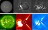 |
Fig. 1. Top panel: (left to right) Hα filtergram from the Kanzelhöhe Solar Observatory showing eruptive filament (indicated by arrow), solar filament eruption at 07:36 UT with a flare and at 08:14 UT from Udaipur Solar Observatory on 18 November 2003. Bottom panel: Temporal evolution of associated CME in SOHO EIT, LASCO C2 and C3 field of view on 18 November 2003. |
3.1.1. In situ ICME observations
The magnetic and plasma properties shown in Figures 2 and 3 respectively correspond to a magnetic cloud which originated on 18 November with a flare-associated filament eruption. In situ observations were taken during the interval from 19–22 November 2003 from Wind spacecraft. The three part structure of the CME as seen in LASCO/C2 observations (10:26 UT on 18 November) arrived at 1 AU with a forward shock indicated in both figures with a red line, followed by sheath and the cloud region whose front and rear boundaries are marked by blue lines. Wind detected a shock at 08:06 UT on 20 November with abrupt increase in magnetic and plasma parameters. Magnitude of magnetic field increased from 9 to 16 nT with increase in bulk velocity from 444 to 546 km s−1. Simultaneously, proton density rose from 10 to 14 n/cc while temperature jumped from 0.5 to 2.4 × 10⁵ K (Fig. 3), at the time of shock. The observed proton temperature is compared with 0.5 Texp (half-magnitude of computed expected temperature), computed from (4)
(4)
 (5)(Lopez & Freeman 1986; Lopez 1987), where Vsw is the solar wind bulk velocity. These were checked as a signature of ICMEs and were found consistent with previously reported cases (Gosling et al. 1973; Richardson & Cane 1995). Sheath region embedded in between shock and cloud structure can be identified by compressed magnetic field and plasma parameters with high proton temperature. The magnetic cloud arriving at 10:43 UT on 20 November is clearly distinguished by its relatively high magnetic field strength (B), smooth rotation of elevation angle (θ) from north to south and low electron and proton temperatures (Fig. 2). The beginning of the cloud is marked by drop in plasma beta below unity (β < 1) showing the dominance of magnetic pressure in the region. With the magnetic cloud arrival, the magnetic field strength rises from 37 to a peak value of 58 nT, along with a drop in temperature from 2.6 × 10⁵ K to 1.3 × 10⁵ K. The magnetic cloud resulted in a large geomagnetic storm with Dst ≅ −422 nT.
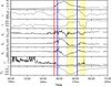 |
Fig. 2. A plot of interplanetary magnetic field parameters from 19 to 22 November 2003. From top to bottom are plotted the magnetic field strength (B), the elevation (θ) and azimuth (ϕ) of the magnetic field direction, three-dimensional magnetic field components (Bx, By, Bz), plasma beta obtained from Wind spacecraft and 1-h averaged Dst index. Red line indicates the shock while the region between blue lines is magnetic cloud. Time is plotted in hours starting from 19 November, 00:00 h. |
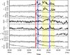 |
Fig. 3. Measurements of proton density (ρp), electron density (ρe), proton thermal velocity (Vth), electron temperature anisotropy, proton temperature anisotropy, electron temperature (Te), proton temperature (Tp) and solar wind bulk velocity (V) obtained from Wind spacecraft. Red line indicates the shock while the region between blue lines is magnetic cloud. The yellow-shaded region is filament plasma, indicated by high density (proton and electron) and low temperatures. |
The bulk velocity drops from 688 to 538 km s−1 (Fig. 3) during the cloud interval, indicating an expansion in cloud with expansion velocity (Zurbuchen & Richardson 2006) Vexp = 75 km s−1 and an average transverse velocity of ≈613 km s−1. The presence of flux rope can also be inferred from the bipolar By and Bz components of the magnetic field. The Bx component points from the spacecraft toward the Sun while By points in the ecliptic plane normal to Bx. The Bz component is normal to the ecliptic plane toward the north pole. In this case, the By component varies from +45 nT (at 13:30 UT) to −30 nT (at 20:00 UT) on 20 November. Similarly, Bz component varies from +37 nT (at 11:15 UT) to −47 nT (at 16:00 UT) on 20 November. End of cloud structure is determined by increase in magnitude of β over unity at 01:17 UT on 21 November 2003.
3.1.2. Identification of filament plasma
3.1.2.1. Magnetic and plasma signatures
Wind detected high proton densities with low temperatures indicating fragmented filamentary material both within and outside the magnetic cloud (shown as yellow-shaded regions in Fig. 3). Inside the cloud region, the filament plasma arrives at Wind on 20 November with sudden rise in proton density from 9 to 22 n/cc. The structure with peak proton density of 26 n/cc passed the spacecraft, lying over the bipolar By and Bz magnetic field components. This feature is consistent with solar disk observations where the filament is seen to be lying along the inversion line between opposite field polarities. Also enhancements in electron densities were observed in the region where the peak density is about 59 n/cc. Proton thermal velocities show depressions in the filament plasma region with a value of ≈38 km s−1. The trailing fragment of filament plasma arrives in the interval from 03:12 UT to 06:58 UT on 21 November, following the magnetic cloud. Here, proton densities attain a maximum value of 17 n/cc with temperature of ≈8.0 × 10⁴ K. Similar trend is observed with electron densities which rise to 44 n/cc and temperature of 1.0 × 10⁵ K in the region. The temperature anisotropy (T⊥/T||) observations (Bame et al. 1975; Marsch et al. 1982; Feldman et al. 1996; Neugebauer et al. 2001) are supposed to be caused by scattering due to Alfven-cyclotron fluctuations (Marsch & Tu 2001; Tu & Marsch 2002; Marsch et al. 2004). In this analysis, the proton temperature anisotropies were found higher than unity (T⊥/T|| > 1) throughout the magnetic cloud and filament regions, while electron temperature anisotropy magnitudes were lower than unity in magnetic cloud region but elevate over unity in filament region during the intervals 18:22 UT on 20 November to 02:00 UT on 21 November and 04:14 UT to 06:07 UT on 21 November.
The thermal velocity features of plasma components were computed from the data obtained by Wind and ACE spacecraft. Depressions in parallel component of thermal velocity (Fig. 4) of proton (SWEPAM/ACE) are observed from 14:06 UT to 15:26 UT in magnetic cloud region with a minimum value of about 25 km s−1. Similar trend is observed in trailing plasma region from 02:48 UT to 03:42 UT on 21 November with an average magnitude of ≈34 km s−1. The perpendicular component of proton thermal velocity (SWEPAM/ACE) has a lower magnitude as compared to parallel component of thermal velocity (Vth⊥ < Vth||), except during the interval 01:22–02:00 UT on 21 November. The perpendicular proton thermal velocity shows depressions from 14:00 UT to 15:00 UT in cloud region with an observed minimum of 24 km s−1 at 14:32 UT. During the trailing plasma region, the thermal velocity shows lower magnitude from 03:00 UT to 07:49 UT on 21 November while having a minimum value ≈17 km s−1. Thermal velocity for alpha particle (Fig. 4) is computed from data obtained by 3DP/Wind during the interval 19–22 November 2003. It shows depressions from 14:51 UT (on 20 November) to 00:55 UT (on 21 November) with a minimum ≈9 km s−1 (at 15:09 UT on 20 November). This trend is also observed from 03:00 UT to 07:00 UT on 21 November in trailing plasma region where it shows a minimum ≈8 km s−1.
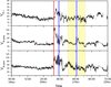 |
Fig. 4. Measurements of He2+ thermal velocity (km s−1) from 3DP/Wind data. Perpendicular (Vthperp) and parallel (Vthpara) components of proton thermal velocity (km s−1) from data by SWEPAM/ACE during the interval 19–22 November 2003. Shaded portion is identified filament plasma. |
Thermal velocities (Fig. 5) of helium (He2+), carbon (C5+), oxygen (O7+) and iron (Fe10+) ions are taken from SWICS/ACE data from 19 to 22 November 2003. Helium ion (He2++) thermal velocity shows depressions during the interval 18:30 UT (on 20 November) to 00:30 UT (on 21 November) with a minimum 24 km s−1 and also from 01:30 UT to 04:30 UT on 21 November as a part of trailing filament plasma region with a minimum magnitude of 27 km s−1. Similar trend is observed in carbon (C5+) thermal velocity which lowers during the interval from 18:30 UT to 22:30 UT on 20 November in magnetic cloud structure with a minimum 16 km s−1. During the trailing plasma region, its magnitude shows depressions from 02:30 UT to 04:30 UT on 21 November with a minimum of ≈12 km s−1. Oxygen (O7+) thermal velocity drops from 19:30 UT to 22:30 UT on 20 November with an average value of ≈18 km s−1 in magnetic cloud while a minimum of ≈16 km s−1 in the trailing region is believed to be associated with filament plasma. Iron (Fe10+) thermal velocities are available with data gaps during observation period. From the data available, it is found that the magnitude of iron thermal velocity is ≈26 km s−1 at 19:30 UT on 20 November within the magnetic cloud region while ≈22 km s−1 at 04:30 UT on 22 November as a part of trailing plasma region.
 |
Fig. 5. Plot showing measurements of (top to bottom); iron (Fe10+), oxygen (O7+), carbon (C5+) and helium (He2++) thermal velocities from SWICS/ACE data. All velocities are expressed in km s−1. |
Figure 6 shows the deviations in RMS values for thermal velocity, temperature, bulk velocity and magnetic field. Thermal velocity deviations acquire nearly constant negative values at 17:00 UT on 20 November, lasting until 00:45 UT on 21 November. Depressions are also seen at 03:00 UT to 08:00 UT on 21 November. Similar trend is observed in RMS deviations of temperature which decrease at 17:00 UT on 20 November to 01:00 UT on 21 November and 03:00 UT to 08:00 UT on 21 November. The bulk velocity also shows a decrease in RMS deviation from 18:30 UT to 20:30 UT on 20 November and from 03:00 UT to 06:10 UT on 21 November, while magnetic field RMS values decrease and remain steady from 18:30 UT on 20 November to 00:45 UT on 21 November followed by depressions on 04:30 UT to 07:10 UT on 21 November indicating the presence of cold filament plasma.
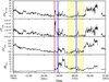 |
Fig. 6. RMS deviations of plasma and magnetic parameters from data obtained from Wind in November 2003, event. |
Data from Wind/SWE, Wind/3DP and Wind/MFI instruments were used to compute thermal (electron + proton) and magnetic pressures (B2/8π) during the interval 12:00–18:00 UT on 20 November and 02:00–04:00 UT on 21 November (Fig. 7). Microscale structures of the order of few minutes were observed on 20 and 21 November as a part of magnetic cloud and trailing region. On 20 November, two structures were identified during 13:00–13:15 and 16:20–16:40 UT followed by more structures on 21 November at 01:10–01:30 UT and 02:00–02:10 UT.
 |
Fig. 7. Plot for computed plasma pressure and magnetic pressure with anti-correlations indicated by arrows during interval 12:00–18:00 UT on 20 November 2003. All parameters are expressed in units of 10−10 dyn cm−2. |
Total pressure remained constant during the observed PBS with an error of ≤7% resulting due to absence of the contribution by alpha particles (Burlaga et al. 1990). Square of magnitude of magnetic field strength (B2) is plotted with proton density from 1 min averaged data and found to have a negative slope during intervals of PBS. Figure 8 shows plot of B2 versus proton density for intervals 13:00–13:15 UT on 20 November, with the regression coefficient (R = −0.93).
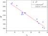 |
Fig. 8. Plot showing square of magnetic field strength (B) versus proton density (ρp) for time intervals during 20 November 2003. |
3.1.2.2. Compositional signatures
Figure 9 shows plots of average carbon, oxygen and iron charge states along with alpha-to-proton ratio obtained from the hourly average data from SWICS instrument onboard ACE spacecraft. The region as identified to be associated with filamentary plasma passed the spacecraft during interval 17:00–22:00 UT on 20 November and 02:30 UT–05:30 UT on 21 November, showing a decrease in carbon and oxygen charge states. Carbon charge state dips to 4.8 as compared to an average 5.5 in ambient plasma while oxygen charge state gets a minimum value of 6.0 within the magnetic cloud region and about 6.2 in the plasma trailing the magnetic cloud on 21 November. The iron charge state remains nearly constant. The region is also associated with increase in proton, electron, ion and helium densities. The solar wind originates from open magnetic field regions (Ogilvie & Hirshberg 1974) of the corona and has He2++/He2+ ratio at about 0.05 in fast wind and even lower in slow wind (von Steiger et al. 1995). CMEs associated with filament eruptions originate from closed field regions and can have up to 30% enhancement in helium abundances (Galvin 1997). Alpha-to-proton ratio is nearly three times in the filamentary plasma region from 17:00 to 22:00 UT on 20 November in magnetic cloud. The observed elemental charge states (C5+, O5+, Fe11+) are also two to three times higher as compared to the compositional signatures for prominence plasma (C5+, O2+, Fe4+) reported by Lepri & Zurbuchen (2010), which is possibly due to eruption of filament with flare.
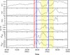 |
Fig. 9. Compositional signatures of filament plasma from 1-h averaged ACE/SWICS data from 19 to 22 November 2003. Top to bottom: average charge distribution (carbon, oxygen, iron), alpha-to-proton ratio, ion density and helium density. |
Measurements of He+ and He++ in November 2003 were made using data from CELIAS/STOF instrument onboard SOHO spacecraft and are shown in Figure 10. The count rates of He+ and He++ are plotted from 16–24 November 2003. Count rates for He+ and He++ are significantly higher on 20 November, along with the high count rates of He+/He++ ratio which corresponds to the filamentary material. CELIAS/STOF recorded a maximum 53 counts for He+, 155 counts for He++ and a ratio 1.2 for He+/He++ within magnetic cloud region on 20 November. In combination with other plasma features, these provide an important clue to associate magnetic cloud with prominence plasma.
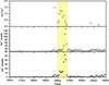 |
Fig. 10. Helium count rates and ratio from CELIAS/STOF onboard SOHO for 20 November 2003 ICME. Count rates in 100–300 keV energy range are marked as star for He+ counts, triangle for He++ counts and circles for the He+/He++ ratio (courtesy: Dr. Martin Hilchenbach). |
The variation in charge state ratios of carbon and oxygen ions was also studied from SWICS/ACE 1-h averaged data during the interval 19–22 November 2003. Figure 11 shows the passage of plasma associated with filament, during the interval 16:30–23:30 UT on 20 November and 01:30–05:30 UT on 21 November 2003. In this interval, the C6/C5 ratio drops below unity with a minimum value 0.12 inside the cloud and a ratio of 0.16 in trailing plasma structure. Similar trend is observed in oxygen charge state ratios (O7/O6) which acquires a minimum of about 0.10 (at 17:30 UT on 20 November) while 0.26 (at 02:30 UT on 21 November) in trailing region behind the magnetic cloud. The Fe/O ratio gets elevated in filament plasma and reaches a maximum of about 0.16 in magnetic cloud and 0.21 in trailing plasma as compared to 0.02 in ambient plasma. The enhancement is around 8 times in cloud region and 10.5 times for plasma trailing the magnetic cloud.
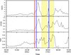 |
Fig. 11. Charge state ratios of carbon and oxygen ions with Fe/O ratio from 19 to 22 November 2003 obtained from SWICS/ACE −1 h resolution data. |
Corresponding freezed-in temperatures for observed charge state ratios were obtained numerically using the relation given by Hundhausen et al. (1968a, 1968b) and ionization and recombination rate coefficients given by Shull & van Steenberg (1982). For carbon charge state ratio of 0.12 in filamentary plasma region, the computed freezed-in temperature is found to be 5.85 × 10⁵ K, while for oxygen charge state ratio of 0.10, the freezed-in temperature is 2.23 × 10⁵ K.
3.2. 1 August 2010 event
Two ICMEs were detected by Wind spacecraft at 04:30 UT (MC1) and 10:32 UT (MC2) on 4 August 2010. These were associated with two filament eruptions observed on 1 August 2010. Hα solar disk observations show a polar crown filament at AR1092 in western hemisphere, stretching from N60W0 to N30W50 while the other at N35W0. Both these filaments are marked as northern (NF) and southern (SF) filaments in Figure 12. The northern filament lifted off from solar surface at 09:30 UT and is observed by SDO/AIA (Lemen et al. 2011) while the southern filament erupted at 22:24 UT and was seen in STEREO-A/COR2 (Howard et al. 2008) images. The interplanetary dynamics of associated CMEs have been studied by Harrison et al. (2012) and Temmer et al. (2012).
 |
Fig. 12. (Left to right) Hα filtergram from the Kanzelhöhe Solar Observatory showing eruptive filaments (indicated as NF and SF), temporal evolution of associated CME in SOHO-EIT, STEREO-A/COR2, LASCO-C3 on 1 August 2010. |
3.2.1. In situ ICME observations
Magnetic and plasma observations taken from Wind spacecraft during 3–5 August 2010 indicate passage of two consecutive magnetic clouds following a shock (S) and sheath structure shown in Figures 13 and 14, identified from magnetic and plasma parameters with one-minute resolution data. Diagnostics of magnetic and plasma features indicate a shock arriving at Wind at 17:47 UT on 3 August. With the shock, magnetic field strength jumped from approx 3 to 8 nT while bulk velocity increased from 414 to 472 km s−1. Also, proton density rises from 4 to 8.5 n/cc with rise in temperature from 1.9 × 10⁴ to 3.4 × 10⁴ K. The shock related-jump conditions were also observed in proton thermal velocity, electron density, Bx and Bz components of magnetic field vector. Following the shock is the sheath region, identified by compressions in magnetic and plasma parameters. During this interval, proton temperature increased up to 4.5 × 10⁵ K with fluctuating magnetic field strength around 11 nT and the ICME also caused a moderate geomagnetic storm (Gonzalez et al. 1994) which reached to a Dst value of −64 nT.
 |
Fig. 13. A plot of magnetic field parameters from 3 to 5 August (12:00 UT), 2010. Top to bottom: the magnetic field strength (B), the elevation (θ) and azimuth (ϕ) of the magnetic field direction, three-dimensional magnetic field components (Bx, By, Bz), plasma beta obtain from Wind spacecraft and 1-h averaged Dst index. Red line indicates the shock while the region between blue lines is first magnetic cloud (MC1) followed by second magnetic cloud (MC2) shown between green lines. |
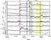 |
Fig. 14. Measurements of proton density, electron density, proton thermal velocity (Vth), electron temperature anisotropy, proton temperature anisotropy, electron temperature (Te), proton temperature (Tp) and solar wind bulk velocity (V) obtained from Wind spacecraft for 4 August ICME. |
3.2.2. Identification of filament plasma
3.2.2.1. Magnetic and plasma signatures
The shock-sheath region is followed by a magnetic cloud (MC1) which resulted from a polar filament eruption on 1 August 2010 as observed by STEREO-A/COR2 (09:54 UT). MC1 passed during the interval from 04:20 to 08:17 UT on 4 August. Front boundary of the cloud is marked with a drop in proton temperature from 2.7 to 2.3 × 10⁵ K and in plasma β from 2.22 to 0.77. The peak value of magnetic field reached a maximum 18 nT with proton temperature 1.01 × 10⁵ K and electron density peaked at about 16 n/cc. The bulk velocity changed from 583 to 576 km s−1 during the cloud interval, indicating an expanding cloud structure. The expanding velocity (Vexp) was found to be 3.5 km s−1 with a transverse velocity ≈580 km s−1. Magnetic field components showed a change from negative to positive values within the cloud. Bz changed from −10 (at 03:53 UT on 4 August) to 11 nT (at 08:49 UT on 4 August) with similar changes in By component which varies from −15 (at 06:24 UT on 4 August) to 11 nT (at 08:49 UT on 4 August). Elevation angle θ changes from 21.2° at 03:30 UT to 53.6° at 08:30 UT on 4 August while azimuth angle ϕ varies from 270° at 03:30 UT to 98.7° at 08:30 UT on 4 August, indicating a west-east orientation in magnetic flux rope configuration. The end of the cloud is marked with increase in magnitude of plasma β over unity at 08:17 UT on 4 August.
Second magnetic cloud (MC2) closely followed the first cloud (MC1) and arrived at 10:32 UT on 4 August with rise in magnetic field and a drop in plasma β below unity. This cloud is associated with filament eruption (SF) on 1 August (Fig. 12) and was a CME in STEREO-A/COR2 at 22:24 UT. The magnetic field vector rises up to 14 nT in cloud region with average proton and electron temperatures 1.84 × 10⁴ K and 1.45 × 10⁵ K respectively. The elevation angle varies from −6.6° to −67.7° while ϕ changed from 234.3° to 321.1° in cloud interval. The By component changes from −11 nT (at 10:33 UT) to −2 nT (at 22:51 UT) while Bz remains negative with very low variance in cloud region, indicating that the spacecraft might have had a glancing encounter with the cloud. Bulk velocity during the cloud interval declines from 592 to 509 km s−1 indicating an expanding structure with velocity (Vexp) approx 41 km s−1 and a transverse velocity approx 550 km s−1.
Plasma and magnetic observations confirm the presence of filament plasma at the rear of magnetic clouds (MC1 and MC2). High density and low temperature plasma passes the spacecraft at the rear boundary of MC1 during the interval from 07:11 UT to 09:30 UT on 4 August. This consists of high proton, electron and ion densities with low temperature of the order of 104 K. Peak value of proton density reaches 24 n/cc with proton temperature of about 7.19 × 10⁴ K and electron temperature of about 1.37 × 10⁵ K with peak electron density about 17 n/cc. By component shows a change from −12 to 12 nT in this region indicating a flux rope configuration. Presence of filamentary plasma over flux rope structure is consistent with the fact that filaments form over the inversion line between opposite magnetic polarities (Martens & Kuin 1989; Martens & Zwaan 2001).
Also, regions with high density and low temperature were observed in rear of MC2 during the interval 13:12 UT on 4 August to 01:45 UT on 5 August. This region appears like a diffused plasma section of the filament material encountered by Wind. Peak proton density reaches a value of 7 n/cc with extremely low temperature 1.6 × 10⁴. Also, low values of electron densities are recorded with peak at ≈4 n/cc and temperature 1.4 × 10⁵ K. Electron anisotropies remain below unity during entire filament plasma and cloud region in MC1 while proton temperature anisotropies were above unity during interval 04:30–06:30 UT in early part of MC1, but were below unity in filament plasma region. In case of second magnetic cloud (MC2), the electron anisotropies are well below unity but proton anisotropies fluctuated around unity till 12:30 UT. It increased above unity in the rear of MC2 at 23:30 UT indicating presence of Alfven-cyclotron fluctuations (Gary et al. 2006).
The plasma and magnetic signatures for filament plasma identification are conspicuously visible for first magnetic cloud (MC1) but not in second magnetic cloud (MC2). The possible explanation could be the location of spacecraft (Wind and ACE) which made a glancing encounter with one of the flank regions of the MC2. This is also confirmed by the Grad-Shafranov reconstruction of the magnetic cloud by Möstl et al. (2012) and supports the view that the spacecraft location plays a key role in identification of ICME structures and the nature of plasma within (Gopalswamy 2006). In this case, it seems that the spacecraft trajectory encountered the MC1 axis while skimmed one of the flanks of MC2, indicated by low varying magnetic field components and low density plasma; related to filament eruption on 1 August 2010.
Data from SWEPAM/ACE, 3DP/Wind and SWICS/ACE have been used to study the nature of thermal velocities of ionic species during the ICME (MC1 and MC2) interval. The computed thermal velocity component in parallel direction (Fig. 15) shows a decreasing trend starting from 18:00 UT on 4 August until 00:30 UT on 5 August. At the rear boundary of MC1, the parallel proton thermal velocity drops from 64 to 18 km s−1, indicating the presence of cold filament material. In the second magnetic cloud (MC2), its value is lowest and approx 24 km s−1. The perpendicular component of proton thermal velocity shows depressions during the interval 13:30–23:45 UT on 4 August and had minimum of about ≈16 km s−1. The alpha thermal velocity (Fig. 15) computed from data obtained by 3DP/Wind instrument shows a high magnitude, nearly constant thermal velocity during the interval 18:00–23:00 UT on 4 August with an average magnitude ≈39 km s−1 in MC2. At the rear boundary MC1, the magnitude suddenly drops from ≈74 to 42 km s−1 at 09:50 UT on 4 August indicating the presence of low temperature plasma.
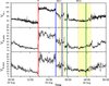 |
Fig. 15. Measurements of He++ thermal velocity (km s−1) from 3DP/Wind data. Perpendicular (Vthperp) and parallel (Vthpara) components of proton thermal velocity (km s−1) from data by SWEPAM/ACE during the interval 3–5 (12:00 UT) August 2010. Shaded portion is filament plasma region. |
SWICS/ACE observations for ionic thermal velocities (Fig. 16) show depressions in helium thermal velocity from 15:00 UT until 23:00 UT on 4 August with a minimum ≈11 km s−1. There were data gaps in observed carbon thermal velocities but with the available data, it has been observed that the magnitude drops during 10:00 UT (on 4 August)–00:00 UT (on 5 August) with a minimum value ≈7 km s−1. The oxygen thermal velocity shows low magnitude during 12:00 UT (on 4 August)–00:00 UT (on 5 August) with a minimum observed value of about ≈7 km s−1. At the rear boundary of MC1, the magnitude of oxygen thermal velocity drops to ≈18 km s−1. Data for iron thermal velocities are not available during the observation period though a magnitude of ≈11 km s−1 is observed at rear end of MC1.
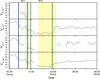 |
Fig. 16. (top to bottom) Plot showing measurements of; iron (Fe10+), oxygen (O7+), carbon (C5+) and helium (He++) thermal velocities from SWICS/ACE instruments. All velocities are expressed in km s−1. |
Figure 17 shows plots of deviations in temperature, magnetic field with bulk and thermal velocities, calculated from Wind data. Decrease in the RMS deviations of these parameters is taken as signatures of filamentary material along with other plasma and magnetic observations. The depressions indicate the presence of prominence plasma at rear of MC1 and MC2 arriving on 4 August at 04:30 UT and 10:32 UT respectively.
 |
Fig. 17. RMS deviations in (top to bottom) thermal velocity, temperature, bulk velocity, magnetic field from 3 August (00:00) to 5 August (12:00), 2010 ICMEs. |
RMS deviations in magnetic field reached negative values from 07:05 UT to 09:02 UT on 4 August and from 13:00 UT on 4 August till 01:00 UT on early 5 August. Similar observations were seen in temperature deviations which were low and nearly constant from 13:00 UT (4 August) to 02:00 UT (5 August). Bulk and thermal velocity deviations are also low during same region. These observations along with other magnetic and plasma signatures indicate the presence of cold filamentary plasma.
Figure 18 shows a mesoscale plot of proton, electron, thermal, magnetic and total pressure over an interval of day, computed by Wind and ACE data. The features we are interested in are appeared in magnetic clouds (MC1 and MC2) at 04:20 UT and 10:32 UT respectively on 4 August. The microstructures can be seen over a scale of 10–60 min.
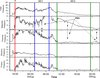 |
Fig. 18. Plot for computed plasma pressure and magnetic pressure with anti-correlations during interval 15:00 UT on 3 August 2010 to 03:00 UT on 5 August 2010. All parameters are expressed in units of 10−10 dyn cm−2. |
Square of magnitude of magnetic field strength (B2) is plotted with proton density and found to have a negative slope during intervals of PBS. Figure 19 shows plots of B2 versus proton density for interval 06:30–07:30 UT on 4 August 2010, with regression coefficient (R = −0.92).
 |
Fig. 19. Plot between square of magnetic field strength versus proton density for time interval 06:30–07:00 UT on 4 August 2010. |
3.2.2.2. Compositional signatures
Presence of filamentary plasma as low charge state species is observed in datasets from SWICS/ACE. Plots of hourly averaged charge state distribution from 4 to 7 August 2010 in Figure 20 show low charge states of carbon, oxygen and iron with high ion density during the intervals in magnetic clouds, believed to be associated with filament eruption. The filamentary plasma arrived as a part of the magnetic cloud (MC1) from 06:00–09:00 UT on 4 August and also in rear of second magnetic cloud (MC2) from 13:00 UT on 4 August to 03:00 UT on 5 August. In the regions with elevated ion, electron and proton densities, the charge state of carbon gets as low as 4.3 while the oxygen and iron charge states decreased to 5.7 and 8.2 respectively in magnetic clouds (MC1 and MC2). He++/H+ ratio attains a peak in MC1 with magnitude 0.09. The He++/H+ ratio in solar wind also shows solar cycle dependencies (Ogilvie & Hirshberg 1974; Feldman et al. 1978; Neugebauer 1981; Ogilvie et al. 1989), which leads to a decreased proton flux at 2.5 R⊙ during solar minimum. This reduction of the proton flux decreases the efficiency of the Coulomb drag and reduces the He++/H+ ratio in solar wind (Aellig et al. 2001). Here, the average He++/H+ ratio in ambient solar wind is 0.01–0.02. The region in MC2 shows an elevated plateau of proton and electron densities, implying a diffused plasma cloud of filament plasma.
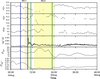 |
Fig. 20. Compositional signatures of filament plasma from 1-h averaged ACE/SWICS data from 4 to 6 August 2010. Average charge distribution (carbon, oxygen, iron), 1-min averaged alpha to proton ratio from 3DP/Wind, ion density and helium density are plotted from top to bottom. |
Further, the He+ and He++ count rates from CELIAS/STOF show (Fig. 21) a sharp increase on 3 August with high He+/He++ ratio. Instrument has detected two counts for He+ ion while six counts for He++ ions and a He+/He++ ratio of 3. It is here important to mention that the sensitivity of the STOF instrument on CELIAS/SOHO has degraded significantly since its launch. In this case, the count statistics is poor as compared to November 2003 event (M. Hilchenbach, priv. comm.).
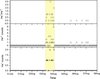 |
Fig. 21. Helium count rates and ratio from CELIAS/STOF onboard SOHO from 31 July to 8 August 2010. Filamentary plasma is estimated to arrive on 3–4 August. Count rates in 100–300 keV energy range are marked as star for He+ counts, triangle for He++ counts and circles for the He+/He++ ratio (courtesy: Dr. Martin Hilchenbach). |
The ratio of charge states (Fig. 22) of carbon and oxygen ions was taken by SWICS/ACE with data gaps in MC2 region. Thus, the freeze-in properties are only determined for MC1 where the C6/C5 ratio drops to 0.15 in filament plasma region. Similar trend is observed with oxygen charge state ratios which shows a dip to 0.1 in filament region.
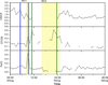 |
Fig. 22. Charge state ratios of carbon, oxygen ions and Fe/O ratio from 4 to 6 August 2010 obtained from SWICS/ACE −1 h resolution data. |
The Fe/O ratio peaked at rear boundary of MC1 with a value around 4.2 which is about ≈5 times higher than that in ambient plasma (0.08). For a carbon charge state ratio of 0.15 in filament plasma region, the computed freeze-in temperature is found to be 6.02 × 10⁵ K while for oxygen charge state ratio of 0.18, the computed temperature is 5.74 × 10⁵ K.
4. Discussion
In this paper, we detected the presence of filament plasma in two ICMEs observed during different phases of solar cycle. Magnetic and plasma parameters were used along with compositional signatures to investigate the filament ejecta at 1 AU. We studied magnetic field signatures to identify magnetic clouds and flux rope configuration therein. The presence of filament plasma over polarity inversion line is consistent with filament models from Martens & Kuin (1989) and Martens & Zwaan (2001). Plasma properties for filament plasma such as low temperature, high proton and electron densities coincided with pressure balanced regions in magnetic clouds. Compositional signatures such as depressed ion charge states and high ion and helium densities and presence of He+ ions were also observed in filament plasma region. Studied ICMEs appear to have a mixture of cold and hot plasma, which were also reported in other in situ plasma studies by Gloeckler et al. (1998) and in combination with presence of He+ ions by Gosling et al. (1980). The rarity of finding cold, low charge state ions at 1 AU as filament plasma suggests partial ionization of elements during transit through corona and development of magnetically confined plasmoids of mixed charge states (Neukomm & Bochsler 1996; Skoug et al. 1999). It is thus possible that filament material is regularly observed in ICMEs at 1 AU, but is not recognized as such because it is no longer distinguished as ionizationally cold (Skoug et al. 1999). Signatures were also seen as depressions in root mean square deviations in ICMEs. Magnetic and plasma parameters such as magnetic field strength (B), thermal (Vth) and bulk (V) velocities and temperature showed lower magnitude of RMS deviations in filament plasma regions. The observed signatures can be summarized in Table 1.
Summary of plasma and magnetic parameters associated with studied ICMEs. Y = yes, ‘–’ = not observed.
Previously reported cases of filament detection in ICMEs by Burlaga et al. (1998), Gopalswamy et al. (1998), Yao et al. (2010) and Lepri & Zurbuchen (2010) were all focused on identifying and reporting the most ideal cases of filament plasma in ICMEs. Despite the fact that most of the solar eruptions are associated with filaments, only a few of them have been reported to contain cold material with low charge state species. This could possibly be due to location of the spacecraft, single point observations and/or due to heating of filamentary material as a result of a physical mechanism with solar (Filippov & Koutchmy 2002) or in situ origins (Burlaga & Behannon 1987; Burlaga 1995; Smith et al. 2001). The data analysis carried out in this study is limited to a single point observation, whereas ICMEs are three-dimensional structures that can be truly understood only through multipoint observations. The magnetic, plasma and compositional parameters were found to be in the same range despite the fact that the two ICMEs originated from different source regions at different phases of solar cycle. Use of different instruments, data analysis techniques and selection criteria also influences the identification of prominence plasma in ICMEs.
The in situ observations of ICMEs are a consequence of the physical mechanisms of their acceleration and injection into interplanetary medium and transportation along interplanetary magnetic field. In this paper, we have adopted the most practical approach to examine as many signatures as possible and identify the filament plasma based on grouping of several signatures within a certain region which can be assumed to be associated with filamentary plasma. The selected region might have distinct boundaries in plasma, magnetic and other signatures since they arise from different physical mechanisms and travel through different ambient medium at different phases of solar cycle.
Acknowledgments
We would like to thank P. Venkatakrishnan, Bernd Inhester and Shou Yao for useful discussions on the subject. The solar wind data from Wind and ACE spacecraft were obtained from NASA CDAWeb (http://cdaweb.gsfc.nasa.gov). We are grateful to Ruth Skoug for providing plasma data from SWEPAM/ACE, Martin Hilchenbach and Harald Kucharek for providing helium ion data from CELIAS/STOF instrument. The work presented here by R.S. was carried out during his Student Project Traineeship at Udaipur Solar Observatory/Physical Research Laboratory. R.S. also acknowledges financial support from the organizers of SPACE CLIMATE-4 conference to attend the meeting at Goa, during 16–21 January 2011. The work by N.S. partially contributes to the research for European Union Seventh Framework Programme (FP7/2007-2013) for the Coronal Mass Ejections and Solar Energetic Particles (COMESEP) project under Grant Agreement No. 263252.
References
- Aellig, M.R., A.J. Lazarus, and J.T. Steinberg, The solar wind helium abundance: variation with wind speed and the solar cycle, Geophys. Res. Lett., 28 (14), 2767–2770, 2001. [NASA ADS] [CrossRef] [Google Scholar]
- Alexander, D., I.G. Richardson, and T.H. Zurbuchen, A brief history of CME science, Space Sci. Rev., 123, 3–11, 2006. [CrossRef] [Google Scholar]
- Bame, S.J., J.R. Asbridge, W.C. Feldman, M.D. Montgomery, and P.D. Kearney, Solar wind heavy ion abundances, Sol. Phys., 43, 463, 1975. [CrossRef] [Google Scholar]
- Bame, S.J., J.R. Asbridge, W.C. Feldman, E.E. Fenimore, and J.T. Gosling, Solar wind heavy ions from flare heated coronal plasma, Sol. Phys., 62, 179–201, 1979. [CrossRef] [Google Scholar]
- Bothmer, V., and R. Schwenn, Eruptive prominences as sources of magnetic clouds in the solar wind, Space Sci. Rev., 70, 215, 1994. [NASA ADS] [CrossRef] [Google Scholar]
- Brueckner, G.E., R.A. Howard, M.J. Koomen, C.M. Korendyke, D.J. Michels, et al., The large angle spectroscopic coronagraph (LASCO), Sol. Phys., 162, 357, 1995. [NASA ADS] [CrossRef] [Google Scholar]
- Burlaga, L.F., Micro-scale structures in the interplanetary medium, Sol. Phys., 4, 67, 1968. [NASA ADS] [CrossRef] [Google Scholar]
- Burlaga, L.F., Interplanetary Magnetohydrodynamics, Oxford University Press, Oxford, ISBN-0-19-508472-1, 1995. [Google Scholar]
- Burlaga, L.F., and K.W. Behannon, Compound streams, magnetic clouds and major geomagnetic storms, J. Geophys. Res., 92, 5725, 1987. [NASA ADS] [CrossRef] [Google Scholar]
- Burlaga, L.F., and K.W. Ogilvie, Magnetic and thermal pressures in the solar wind, Sol. Phys., 15, 61–71, 1970. [NASA ADS] [CrossRef] [Google Scholar]
- Burlaga, L.F., L.W. Klein, N.R. Sheeley Jr., D.J. Michels, R.A. Howard, M.J. Koomen, R. Schwenn, and H. Rosenbauer, A magnetic cloud and a coronal mass ejection, Geophys. Res. Lett., 9, 317, 1982. [Google Scholar]
- Burlaga, L.F., J.D. Scudder, L.W. Klein, and P.A. Isenberg, Pressure-balanced structures between 1 AU and 24 AU and their implications for solar wind electrons and interstellar pickup ions, J. Geophys. Res., 95, 2229, 1990. [NASA ADS] [CrossRef] [Google Scholar]
- Burlaga, L., R. Fitzenreiter, R. Lepping, K. Ogilvie, A. Szabo, et al., A magnetic cloud containing prominence material: January 1997, J. Geophys. Res., 103 (A1), 277–285, 1998. [NASA ADS] [CrossRef] [Google Scholar]
- Chandra, R., E. Pariat, B. Schmieder, C.H. Mandrini, and W. Uddin, How can a negative magnetic helicity active region generate a positive helicity magnetic cloud? Sol. Phys., 261, 127–148, 2010. [NASA ADS] [CrossRef] [Google Scholar]
- Chandra, R., B. Schmieder, C. Mandrini, P. Demoulin, E. Pariat, et al., Homologous flares and magnetic field topology in active region NOAA 10501 on 20 November 2003, Sol. Phys., 269, 83–104, DOI: 10.1007/s11207-010-9670-9, 2011. [NASA ADS] [CrossRef] [Google Scholar]
- Crooker, N.U., and T.S. Horbury, Solar imprint on ICMEs, their magnetic connectivity and heliospheric evolution, Space Sci. Rev., 123, 93–109, 2006. [Google Scholar]
- Feldman, W.C., J.R. Asbridge, S.J. Bame, and J.T. Gosling, Long-term variations of selected solar wind properties: Imp 6, 7, and 8 results, J. Geophys. Res., 83, 2177–2189, 1978. [Google Scholar]
- Feldman, W.C., B.L. Barraclough, and J.L. Phillips, Constraints on high-speed solar wind structure near its coronal base: a Ulysses perspective, A&A, 316, 355, 1996. [Google Scholar]
- Ferraro, V.C.A., and C. Plumpton, An Introduction to Magneto-Fluid Dynamics, Clarendon Press, Oxford, 1966. [Google Scholar]
- Filippov, B., and S. Koutchmy, About the prominence heating mechanisms during its eruptive phase, Sol. Phys., 208, 283–295, 2002. [NASA ADS] [CrossRef] [Google Scholar]
- Forsyth, R.J., V. Bothmer, C. Cid, N.U. Crooker, T.S. Horbury, et al., ICMEs in the inner heliosphere: origin, evolution and propagation effects, Space Sci. Rev., 123, 383–416, 2006. [NASA ADS] [CrossRef] [Google Scholar]
- Galvin, A.B., Minor ion composition in CME-related solar wind, In Coronal Mass Ejections, eds. N., Crooker, J.A. Joselyn, and J. Feynmann, AGU, Washington, 253, 1997. [CrossRef] [Google Scholar]
- Gary, S.P., L. Yin, D. Winske, J.T. Steinberg, and R.M. Skoug, Solar wind ion scattering by Alfven-cyclotron fluctuations: ion temperature anisotropies versus relative alpha particle densities, New J. Phys., 8, 17, 2006. [CrossRef] [Google Scholar]
- Geiss, J., G. Gloeckler, R. von Steiger, H. Balsiger, L.A. Fisk, et al., The southern high-speed stream – results from the SWICS instrument on Ulysses, Science, 268, 1033, 1995. [NASA ADS] [CrossRef] [PubMed] [Google Scholar]
- Gloeckler, G., J. Cain, F.M. Ipavich, E.O. Tums, P. Bedini, et al., Investigation of the composition of solar and interstellar matter using solar wind and pickup ion measurements with SWICS and SWIMS on the ACE spacecraft, Space Sci. Rev., 86, 497, 1998. [NASA ADS] [CrossRef] [Google Scholar]
- Gonzalez, W.D., J.A. Joselyn, Y. Kamide, H.W. Kroehl, G. Rostoker, et al., What is a geomagnetic storm? J. Geophy. Res., 99 A4, 5771–5792, 1994. [Google Scholar]
- Gopalswamy, N., Properties of interplanetary coronal mass ejections, Space Sci. Rev., 124, 145–168, DOI: 10.1007/s 11214-006-9102-1, 2006. [Google Scholar]
- Gopalswamy, N., Y. Hanaoka, T. Kosugi, R.P. Lepping, J.T. Steinberg, et al., On the relationship between coronal mass ejections and magnetic clouds, Geophys. Res. Lett., 25 (14), 2485–2488, 1998. [NASA ADS] [CrossRef] [Google Scholar]
- Gopalswamy, N., S. Yashiro, G. Michalek, H. Xie, R.P. Lepping, and R.A. Howard, Solar source of the largest geomagnetic storm of cycle 23, Geophys. Res. Lett., 32, L12S09, DOI: 10.1029/2004GL021639, 2005. [CrossRef] [Google Scholar]
- Gosling, J.T., V. Pizzo, and S.J. Bame, Anomalously low proton temperatures in the solar wind following interplanetary shock waves – evidence for magnetic bottles? J. Geophys. Res., 78, 2001, 1973. [Google Scholar]
- Gosling, J.T., J.R. Asbridge, S.J. Bame, and W.C. Feldman, Observations of large fluxes of He+ in the solar wind following an interplanetary shock, J. Geophys. Res., 85, 3431, 1980. [CrossRef] [Google Scholar]
- Harrison, R.A., J.A. Davies, C. Möstl, Y. Liu, M. Temmer, et al., An analysis of the origin and propagation of the multiple coronal mass ejection of 2010 August 1, Astrophys. J., 750, 45, DOI: 10.1088/0004-637X/750/1/45, 2012. [Google Scholar]
- Hovestadt, D., M. Hilchenbach, A. Bürgi, B. Klecker, P. Laeverenz, et al., CELIAS – Charge, Element and Isotope Analysis System for SOHO, Sol. Phys., 162, 441, 1995. [NASA ADS] [CrossRef] [Google Scholar]
- Howard, R.A., D.J. Michels, N.R. Sheeley Jr., and M.J. Koomen, The observation of a coronal transient directed at Earth, Astrophys. J., 263, 1982. [Google Scholar]
- Howard, R.A., J.D. Moses, A. Vourlidas, J.S. Newmark, D.G. Socker, et al., Sun earth connection coronal and heliospheric investigation (SECCHI), Space Sci. Rev., 136, 67–115, 2008. [NASA ADS] [CrossRef] [Google Scholar]
- Hu, Q., and B.U.Ö. Sonnerup, Reconstruction of magnetic clouds in the solar wind: orientations and configurations, J. Geophys. Res., 107 (A7), 1142, DOI: 10.1029/2001JA000293, 2002. [CrossRef] [Google Scholar]
- Hudson, H.S., J.L. Bougeret, and J. Burkepile, Coronal mass ejections: overview of observations, Space Sci. Rev., 123, 13, 2006. [NASA ADS] [CrossRef] [Google Scholar]
- Hundhausen, A.J., Coronal expansion and solar wind, Springer-Verlag, New York, 1972. [CrossRef] [Google Scholar]
- Hundhausen, A.J., The origin and propagation of coronal mass ejections, in Solar Wind Six, eds. V.J., Pizzo, T.E. Holzer, and D.G. Sime, Proc, Natl. Cent. for Atmos. Res., Boulder, Colo, p. 181, Tech. Note, 306, 1988. [Google Scholar]
- Hundhausen, A.J., H.E. Gilbert, and S.J. Bame, Ionization state of the interplanetary plasma, J. Geophys. Res., 73, 5485, 1968a. [Google Scholar]
- Hundhausen, A.J., H.E. Gilbert, and S.J. Bame, The state of ionization of oxygen in the solar wind, Astrophys. J., 152, 1968b. [Google Scholar]
- Klein, L.W., and L.F. Burlaga, Interplanetary magnetic cloud at 1 AU, J. Geophys. Res., 87, 613, 1982. [Google Scholar]
- Kumar, P., P.K. Manoharan, and W. Uddin, Multiwavelength study on solar and interplanetary origins of the strongest geomagnetic storm of solar cycle 23, Sol. Phys., 271 (1–2), 149–167, 2011. [NASA ADS] [CrossRef] [Google Scholar]
- Lemen, J.R., A.M. Title, C. Akin, J.F. Drake, D.W. Duncan, et al., Atmospheric imaging assembly (AIA) on the solar dynamics observatory (SDO), Sol. Phys., 275, 17–40, DOI: 10.1007/s11207-011-9776-8, 2011. [Google Scholar]
- Lepping, R.P., M.H. Acuna, L.F. Burlaga, W.M. Farrell, J.A. Slavin, et al., The WIND magnetic field investigation, Space Sci. Rev., 207, 1995. [NASA ADS] [CrossRef] [Google Scholar]
- Lepri, S.T., and T.H. Zurbuchen, Direct observational evidence of filament material within interplanetary coronal mass ejections, Astrophys. J. Lett., 723, 22–27, DOI: 10.1088/2041-8205/723/1/L22, 2010. [CrossRef] [Google Scholar]
- Lopez, R.E., Solar cycle invariance in solar wind proton temperature relationships, J. Geophys. Res., 92 (A10), DOI: 10.1029/JA092iA10p11189, 1987. [CrossRef] [Google Scholar]
- Lopez, R.E., and J.W. Freeman, Solar wind proton temperature-velocity relationship, J. Geophys. Res., 91, 1701–1705, 1986. [NASA ADS] [CrossRef] [Google Scholar]
- Marsch, E., and C.Y., Tu, Evidence for pitch angle diffusion of solar wind protons in resonance with cyclotron waves, J. Geophys. Res., 106, 8357, 2001. [CrossRef] [Google Scholar]
- Marsch, E., K.H. Mühlhäuser, R. Schwenn, H. Rosenbauer, W. Pilipp, and F.M. Neubauer, Solar wind protons: three dimensional velocity distributions and derived plasma parameters measured between 0.3 and 1 AU, J. Geophys. Res., 87 (A1), 52–72, 1982. [NASA ADS] [CrossRef] [Google Scholar]
- Marsch, E., X.Z. Ao, and C.Y. Tu, On the temperature anisotropy of the core part of the proton velocity distribution function in the solar wind, J. Geophys. Res., 109, A04102, DOI: 10.1029/2003JA010330, 2004. [NASA ADS] [CrossRef] [Google Scholar]
- Martens, P.C.H., and N.P.M. Kuin, A circuit model for filament eruptions and two ribbon flares, Sol. Phys., 122, 263–302, 1989. [NASA ADS] [CrossRef] [Google Scholar]
- Martens, P.C., and C. Zwaan, Origin and evolution of filament-prominence systems, Astrophys. J., 558, 872–887, 2001. [Google Scholar]
- Marubashi, K., Structure of interplanetary magnetic clouds and their solar origins, Adv. Space Res., 6 (6), 33, 1986. [Google Scholar]
- McComas, D.J., S.J., Bame, P., Barker, W.C., Feldman, J.L., Phillips, P., Riley, and J.W., Griffee, Solar Wind Electron Proton Alpha Monitor (SWEPAM) for the Advanced Composition Explorer, Space Sci. Rev., 86, 563–612, 1998. [NASA ADS] [CrossRef] [Google Scholar]
- Möstl, C., C. Miklenic, C.J. Farrugia, M. Temmer, A. Veronig, A.B. Galvin, B. Vršnak, and H.K. Biernat, Two-spacecraft reconstruction of a magnetic cloud and comparison to its solar source, Ann. Geophys., 26, 3139–3152, 2008. [CrossRef] [Google Scholar]
- Möstl, C., C.J. Farrugia, E.K.J. Kilpua, L. Jian, and Y. Liu, Multi-point shock and flux rope analysis of multiple interplanetary coronal mass ejections around 2010 August 1 in the inner heliosphere, Astrophys. J., 2012, in press. [Google Scholar]
- Neugebauer, M., Observations of solar wind helium, Fund. Cosmic Phys., 7, 131, 1981. [Google Scholar]
- Neugebauer, M., B.E. Goldstein, D. Winterhalter, E.J. Smith, R.J. MacDowall, and S.P. Gary, Ion distributions in large magnetic holes in the fast solar wind, J. Geophys. Res., 106, 5635, 2001. [NASA ADS] [CrossRef] [Google Scholar]
- Neukomm, R.O., and P. Bochsler, Diagnostics of closed magnetic structures in the solar corona using charge states of helium and of minor ions, Astrophys. J., 465, 462, 1996. [CrossRef] [Google Scholar]
- Ogilvie, K.W., and J. Hirshberg, The solar cycle variation of the solar wind helium abundance, J. Geophys. Res., 79, 4595–4602, 1974. [CrossRef] [Google Scholar]
- Ogilvie, K.W., M.A. Coplan, and P. Bochsler, Solar wind observations with the ion composition instrument aboard the ISEE-3/ICE spacecraft, Sol. Phys., 124, 167–183, 1989. [CrossRef] [Google Scholar]
- Ogilvie, K.W., D.J. Chornay, R.J. Fritzenreiter, F. Hunsaker, J. Keller, et al., SWE, a comprehensive plasma instrument for the WIND spacecraft, Space Sci. Rev., 71, 55, 1995. [NASA ADS] [CrossRef] [Google Scholar]
- Owocki, S.P., and J.D. Scudder, The effect of a non-Maxwellian electron distribution on oxygen and iron ionization balances in the solar wind, Astrophys. J., 270, 758, 1983. [Google Scholar]
- Pudovkin, M.I., S.A. Zaitseva, and E.E. Benevolenska, The structure and parameters of flare streams, J. Geophys. Res., 84 (A11), 6649–6652, DOI: 10.1029/JA084iA11p06649, 1979. [CrossRef] [Google Scholar]
- Richardson, I.G., and H.V. Cane, Regions of abnormally low proton temperature in the solar wind (1965-1991) and their association with ejecta, J. Geophys. Res., 100, 23397–23412, 1995. [NASA ADS] [CrossRef] [Google Scholar]
- Schmieder, B., P. D’emoulin, E. Pariat, T. Török, Molodij, et al., Actors of the main activity in large complex centres during the 23 solar cycle maximum, Adv. Space Res., 47, 2081–2091, DOI: 10.1016/j.asr.2011.02.001, 2011. [NASA ADS] [CrossRef] [Google Scholar]
- Schwenn, R., H. Rosenbauer, and K.H. Mühlhäuser, Singly ionized helium in the driver gas of an interplanetary shock wave, Geophys. Res. Lett., 7 (3), 201–204, 1980. [CrossRef] [Google Scholar]
- Schwenn, R., J.C. Raymond, D. Alexander, A. Ciaravella, N. Gopalswamy, et al., Coronal observations of CMEs: report of Working Group A, Space Sci. Rev., 123, 127–176, 2006. [CrossRef] [Google Scholar]
- Shull, J.M., and M. van Steenberg, The ionization equilibrium of astrophysically abundant elements, Astrophys. J. Suppl., 48, 95, 1982. [CrossRef] [Google Scholar]
- Skoug, R.M., S.J. Bame, W.C. Feldman, J.T. Gosling, D.J. McComas, et al., A prolonged He+ enhancement within a coronal mass ejection in the solar wind, Geophys. Res. Lett., 26 (2), 161–164, DOI: 10.1029/1998GL900207, 1999. [NASA ADS] [CrossRef] [Google Scholar]
- Smith, C.W., J. L’Heureux, N.F. Ness, M.H. Acuna, L.F. Burlaga, and J. Scheifele, The ACE Magnetic Field Experiment, Space Sci. Rev., 86 (1-4), 613–632, 1998. [NASA ADS] [CrossRef] [Google Scholar]
- Smith, C.W., W.H. Matthaeus, G.P. Zank, N.F. Ness, S. Oughton, and J.D. Richardson, Heating of the low-latitude solar wind by dissipation of turbulent magnetic fluctuations, J. Geophys. Res., 106, 8253–8272, 2001. [NASA ADS] [CrossRef] [Google Scholar]
- Srivastava, N., S.K. Mathew, and R.E. Louis, Source region of the 18 November 2003 coronal mass ejection that led to the strongest magnetic storm of cycle 23, J. Geophys. Res., 114, A03107, 2009. [CrossRef] [Google Scholar]
- Temmer, M., B. Vrsnak, T. Rollett, B. Bein, and C.A. de Koning, Characteristics of the kinematics of a coronal mass ejection during the 2010 August 1 CME-CME interaction event, Astrophys. J., 749, 57, DOI: 10.1088/0004-637X/749/1/57, 2012. [Google Scholar]
- Tu, C.Y., and E. Marsch, Anisotropy regulation and plateau formation through pitch angle diffusion of solar wind protons in resonance with cyclotron waves, J. Geophys. Res., 107, 1249, DOI: 10.1029/2001JA000150, 2002. [CrossRef] [Google Scholar]
- von Steiger, R., R.F. Wimmer-Schweingruber, J. Geiss, and G. Gloeckler, Abundance variations in the solar wind, Adv. Space Res., 15 (7), 3–12, 1995. [CrossRef] [Google Scholar]
- Wang, Y., G. Zhou, P. Ye, S. Wang, and J. Wang, A study of the orientation of interplanetary magnetic clouds and solar filaments, Astrophys. J., 651, 1245–1255, 2006. [Google Scholar]
- Wilson, R.M., and E. Hildner, Are interplanetary magnetic clouds manifestations of coronal transients at 1 AU? Sol. Phys., 91, 169, 1984. [CrossRef] [Google Scholar]
- Wilson, R.M., and E. Hildner, On the association of magnetic clouds with disappearing filaments, J. Geophys. Res., 91, 5867, 1986. [CrossRef] [Google Scholar]
- Yao, S., E. Marsch, C.Y. Tu, and R. Schwenn, Identification of prominence ejecta by the proton distribution function and magnetic fine structure in interplanetary coronal mass ejections in the inner heliosphere, J. Geophys. Res., 115, A05103, DOI: 10.1029/2009JA014914, 2010. [CrossRef] [Google Scholar]
- Yurchyshyn, V., Q. Hu, and V. Abramenko, Structure of magnetic fields in NOAA active regions 0486 and 0501 and in the associated interplanetary ejecta, Space Weather, 3, S08C02, 2005. [CrossRef] [Google Scholar]
- Zurbuchen, T.H., and I.G. Richardson, In-situ solar wind and magnetic field signatures of interplanetary coronal mass ejections, Space Sci. Rev., 123, 31–43, DOI: 10.1007/s11214-006-9010-4, 2006. [NASA ADS] [CrossRef] [Google Scholar]
- Zwickl, R.D., J.R. Asbridge, S.J. Bame, W.C. Feldman, J.T. Gosling, and E.J. Smith, Plasma properties of driver gas following interplanetary shocks observed by ISEE3, in Solar Wind Five, ed. M., Neugebauer, NASA Conf. Publ., CP2280, 711–717, 1983. [Google Scholar]
All Tables
Summary of plasma and magnetic parameters associated with studied ICMEs. Y = yes, ‘–’ = not observed.
All Figures
|
Fig. 1. Top panel: (left to right) Hα filtergram from the Kanzelhöhe Solar Observatory showing eruptive filament (indicated by arrow), solar filament eruption at 07:36 UT with a flare and at 08:14 UT from Udaipur Solar Observatory on 18 November 2003. Bottom panel: Temporal evolution of associated CME in SOHO EIT, LASCO C2 and C3 field of view on 18 November 2003. |
| In the text | |
|
Fig. 2. A plot of interplanetary magnetic field parameters from 19 to 22 November 2003. From top to bottom are plotted the magnetic field strength (B), the elevation (θ) and azimuth (ϕ) of the magnetic field direction, three-dimensional magnetic field components (Bx, By, Bz), plasma beta obtained from Wind spacecraft and 1-h averaged Dst index. Red line indicates the shock while the region between blue lines is magnetic cloud. Time is plotted in hours starting from 19 November, 00:00 h. |
| In the text | |
|
Fig. 3. Measurements of proton density (ρp), electron density (ρe), proton thermal velocity (Vth), electron temperature anisotropy, proton temperature anisotropy, electron temperature (Te), proton temperature (Tp) and solar wind bulk velocity (V) obtained from Wind spacecraft. Red line indicates the shock while the region between blue lines is magnetic cloud. The yellow-shaded region is filament plasma, indicated by high density (proton and electron) and low temperatures. |
| In the text | |
|
Fig. 4. Measurements of He2+ thermal velocity (km s−1) from 3DP/Wind data. Perpendicular (Vthperp) and parallel (Vthpara) components of proton thermal velocity (km s−1) from data by SWEPAM/ACE during the interval 19–22 November 2003. Shaded portion is identified filament plasma. |
| In the text | |
|
Fig. 5. Plot showing measurements of (top to bottom); iron (Fe10+), oxygen (O7+), carbon (C5+) and helium (He2++) thermal velocities from SWICS/ACE data. All velocities are expressed in km s−1. |
| In the text | |
|
Fig. 6. RMS deviations of plasma and magnetic parameters from data obtained from Wind in November 2003, event. |
| In the text | |
|
Fig. 7. Plot for computed plasma pressure and magnetic pressure with anti-correlations indicated by arrows during interval 12:00–18:00 UT on 20 November 2003. All parameters are expressed in units of 10−10 dyn cm−2. |
| In the text | |
|
Fig. 8. Plot showing square of magnetic field strength (B) versus proton density (ρp) for time intervals during 20 November 2003. |
| In the text | |
|
Fig. 9. Compositional signatures of filament plasma from 1-h averaged ACE/SWICS data from 19 to 22 November 2003. Top to bottom: average charge distribution (carbon, oxygen, iron), alpha-to-proton ratio, ion density and helium density. |
| In the text | |
|
Fig. 10. Helium count rates and ratio from CELIAS/STOF onboard SOHO for 20 November 2003 ICME. Count rates in 100–300 keV energy range are marked as star for He+ counts, triangle for He++ counts and circles for the He+/He++ ratio (courtesy: Dr. Martin Hilchenbach). |
| In the text | |
|
Fig. 11. Charge state ratios of carbon and oxygen ions with Fe/O ratio from 19 to 22 November 2003 obtained from SWICS/ACE −1 h resolution data. |
| In the text | |
|
Fig. 12. (Left to right) Hα filtergram from the Kanzelhöhe Solar Observatory showing eruptive filaments (indicated as NF and SF), temporal evolution of associated CME in SOHO-EIT, STEREO-A/COR2, LASCO-C3 on 1 August 2010. |
| In the text | |
|
Fig. 13. A plot of magnetic field parameters from 3 to 5 August (12:00 UT), 2010. Top to bottom: the magnetic field strength (B), the elevation (θ) and azimuth (ϕ) of the magnetic field direction, three-dimensional magnetic field components (Bx, By, Bz), plasma beta obtain from Wind spacecraft and 1-h averaged Dst index. Red line indicates the shock while the region between blue lines is first magnetic cloud (MC1) followed by second magnetic cloud (MC2) shown between green lines. |
| In the text | |
|
Fig. 14. Measurements of proton density, electron density, proton thermal velocity (Vth), electron temperature anisotropy, proton temperature anisotropy, electron temperature (Te), proton temperature (Tp) and solar wind bulk velocity (V) obtained from Wind spacecraft for 4 August ICME. |
| In the text | |
|
Fig. 15. Measurements of He++ thermal velocity (km s−1) from 3DP/Wind data. Perpendicular (Vthperp) and parallel (Vthpara) components of proton thermal velocity (km s−1) from data by SWEPAM/ACE during the interval 3–5 (12:00 UT) August 2010. Shaded portion is filament plasma region. |
| In the text | |
|
Fig. 16. (top to bottom) Plot showing measurements of; iron (Fe10+), oxygen (O7+), carbon (C5+) and helium (He++) thermal velocities from SWICS/ACE instruments. All velocities are expressed in km s−1. |
| In the text | |
|
Fig. 17. RMS deviations in (top to bottom) thermal velocity, temperature, bulk velocity, magnetic field from 3 August (00:00) to 5 August (12:00), 2010 ICMEs. |
| In the text | |
|
Fig. 18. Plot for computed plasma pressure and magnetic pressure with anti-correlations during interval 15:00 UT on 3 August 2010 to 03:00 UT on 5 August 2010. All parameters are expressed in units of 10−10 dyn cm−2. |
| In the text | |
|
Fig. 19. Plot between square of magnetic field strength versus proton density for time interval 06:30–07:00 UT on 4 August 2010. |
| In the text | |
|
Fig. 20. Compositional signatures of filament plasma from 1-h averaged ACE/SWICS data from 4 to 6 August 2010. Average charge distribution (carbon, oxygen, iron), 1-min averaged alpha to proton ratio from 3DP/Wind, ion density and helium density are plotted from top to bottom. |
| In the text | |
|
Fig. 21. Helium count rates and ratio from CELIAS/STOF onboard SOHO from 31 July to 8 August 2010. Filamentary plasma is estimated to arrive on 3–4 August. Count rates in 100–300 keV energy range are marked as star for He+ counts, triangle for He++ counts and circles for the He+/He++ ratio (courtesy: Dr. Martin Hilchenbach). |
| In the text | |
|
Fig. 22. Charge state ratios of carbon, oxygen ions and Fe/O ratio from 4 to 6 August 2010 obtained from SWICS/ACE −1 h resolution data. |
| In the text | |
Current usage metrics show cumulative count of Article Views (full-text article views including HTML views, PDF and ePub downloads, according to the available data) and Abstracts Views on Vision4Press platform.
Data correspond to usage on the plateform after 2015. The current usage metrics is available 48-96 hours after online publication and is updated daily on week days.
Initial download of the metrics may take a while.