| Issue |
J. Space Weather Space Clim.
Volume 5, 2015
|
|
|---|---|---|
| Article Number | A9 | |
| Number of page(s) | 15 | |
| DOI | https://doi.org/10.1051/swsc/2015010 | |
| Published online | 17 April 2015 | |
Research Article
Ionospheric forecasts for the European region for space weather applications
National Observatory of Athens, Institute for Astronomy, Astrophysics, Space Applications and Remote Sensing, I. Metaxa & Vas. Pavlou St., 15236
Penteli, Greece
* Corresponding author: This email address is being protected from spambots. You need JavaScript enabled to view it.
Received:
17
September
2014
Accepted:
9
March
2015
Abstract
This paper discusses recent advances in the implementation and validation of the Solar Wind driven autoregression model for Ionospheric short-term Forecast (SWIF) that is running in the European Digital upper Atmosphere Server (DIAS) to release ionospheric forecasting products for the European region. The upgraded implementation plan expands SWIF’s capabilities in the high latitude ionosphere while the extensive validation tests in the two solar cycles 23 and 24 allow the comprehensive analysis of the model’s performance in all terms. Focusing on disturbed conditions, the results demonstrate that SWIF’s alert detection algorithm forecasts the occurrence of ionospheric storm time disturbances with probability of detection up to 98% under intense geomagnetic storm conditions and up to 63% when storms of moderate intensity are also considered. The forecasts show relative improvement over climatology of about 30% in middle-to-low and high latitudes and 40% in middle-to-high latitudes. This indicates that SWIF is able to capture on average more than one third (35%) of the storm-associated ionospheric disturbances. Regarding the accuracy, the averaged mean relative error during storm conditions usually ranges around 20% in middle-to-low and high latitudes and 24% in the middle-to-high latitudes. Our analysis shows clearly that SWIF alert criteria were designed to effectively anticipate the ionospheric storm time effects that occurred under specific interplanetary conditions, e.g., cloud Interplanetary Coronal Mass Ejections (ICMEs) and/or associated sheaths. The results provide valuable input in advancing our ability in predicting the space weather effects in the ionosphere for future developments, and further work is proposed to enhance the model forecasting efficiency to support operational applications.
Key words: Space Weather / Ionosphere / Forecasting / Modelling / Validation
© I. Tsagouri and A. Belehaki, Published by EDP Sciences 2015
 This is an Open Access article distributed under the terms of the Creative Commons Attribution License (http://creativecommons.org/licenses/by/4.0), which permits unrestricted use, distribution, and reproduction in any medium, provided the original work is properly cited.
1. Introduction
Ionospheric forecasting products and services for the European region are routinely provided from the European Digital upper Atmosphere Server (DIAS; Belehaki et al. 2005, 2006, 2007), including alerts and warnings for upcoming foF2 ionospheric storm time disturbances, as well as local and regional forecasts of the foF2 critical frequency up to 24 h ahead in all conditions. The full range of DIAS forecasting services is made available through the implementation of the Solar Wind driven autoregression model for Ionospheric short-term Forecast (SWIF; Tsagouri et al. 2009). Until recently, DIAS forecasting services were designed to cover the needs in the middle-latitude European region up to 60° N (http://dias.space.noa.gr).
Within the Space Situational Awareness (SSA) programme of the European Space Agency (ESA), the DIAS forecasting services have been integrated with ESA/SSA Space Weather Service Network (SWE) to provide ionospheric forecasts over whole Europe, including Scandinavia for HF propagation purposes (http://swe.ssa.esa.int/web/guest/dias-federated) as part of the European Ionosonde Service (EIS). To this effect, DIAS database was enriched to accommodate real-time foF2 observations from two European high latitude ionosondes, Tromso (69.6° N, 19.2° E) and Sodankyla (67.4° N, 26.6° E), and the operational implementation of the SWIF model was expanded accordingly to cover the European high latitudes. This task was supported by extensive validation tests of the model’s performance, which were carefully designed to complement previous efforts in testing the SWIF’s alert detection efficiency for European locations and in quantifying the efficiency of SWIF’s forecasts (e.g., Tsagouri & Belehaki 2008; Tsagouri et al. 2009; Tsagouri 2011). This paper presents the results of this effort, having as the primary objective the compilation of a comprehensive overview of SWIF’s forecasting capabilities over Europe for operational applications. In addition, since SWIF represents an alternative platform for ionospheric forecasting purposes using solar wind parameters as a proxy of the geomagnetic activity level, the systematic evaluation of its performance provides useful insight into understanding and predicting the space weather effects in the ionosphere for future developments.
Following the Introduction, the paper is structured as follows: Section 2 provides an overview of SWIF’s basic concepts and implementation plan with the emphasis on the latest upgrades. The results of the validation tests are provided in Section 3 and they are comprehensively discussed in Section 4. Section 5 summarizes the major conclusions/findings of this work.
2. SWIF’s concept and implementation plan of the enhanced version
The structure of the F-region ionosphere at any given time is determined by a number of influences that may be summarized as follows (Forbes et al. 2000): (a) Solar ionizing flux: the solar photon radiation ionizes the major atmospheric constituents. It varies with the 11-year solar cycle, the quasi-27-day rotation of the Sun, and probably on a day-to-day basis. The solar zenith angle dependence contributes to the diurnal, annual, and semiannual variations in the ionosphere. In addition, solar flux-induced variations in neutral composition, neutral temperatures and winds, and conductivities are also manifested in ionospheric plasma densities. (b) Meteorological influences: processes originating in the lower atmosphere such as fronts, convection systems, sudden stratospheric warmings, etc. (e.g., Kazimirovsky & Kokourov 1991) determine also the state of the ionosphere. The influences on the ionosphere occur mainly as the result of upward-propagating tides, planetary waves, and gravity waves and contribute at significant fraction to the observed variability (e.g., Mendillo et al. 1998). (c) Solar wind conditions: a number of changes in the global structure of the F-region result from the interaction of the solar wind with earth’s magnetic field. The time-dependent response to disturbed solar wind conditions is referred to as an “ionospheric storm”. Variations in the state of the ionosphere associated with storms are primarily connected with transport by electric fields and neutral winds, changes in the neutral composition and structure, and energetic particle precipitation, and they are dependent on local time, latitude, and season (e.g., Prölss 1993).
To support a wide range of forecasting products under all possible ionospheric conditions, SWIF combines two distinct algorithms available for ionospheric storm and non-storm conditions. While the storm algorithm aims to capture the storm-related ionospheric variation, the non-storm component should be able to describe the ionospheric behavior in the rest of the cases capturing the effects of the aforementioned sources. The storm time component is based on the empirical Storm Time Ionospheric Model (STIM; Tsagouri & Belehaki 2006, 2008), which uses the Interplanetary Magnetic Field (IMF) observations at the L1 point from ACE spacecraft as a proxy for upcoming ionospheric foF2 storm time disturbances. The SWIF’s concept is then built upon the STIM’s alert detection algorithm (ADA) that is able to identify storm (alert) conditions and therefore to provide a switch between the two algorithms, the storm and the non-storm one.
The ADA receives as input real-time IMF observations from ACE and applies quantitative criteria to IMF total magnitude B, its rate of change, dB/dt, and IMF-Bz component in order to determine alert conditions and the storm onset at the L1 point. The derivation of the criteria was based on superposed epoch analysis which was carried out over several intense storm events (i.e., min Dst ≤ −100 nT) that occurred in solar cycle 23 (Tsagouri & Belehaki 2006, 2008) and on previously reported empirical relationships that associated the occurrence of intense storm events with IMF southward fields with intensities >10 nT and duration >3 h and high values of IMF intensity, indicating that the interplanetary manifestations of coronal mass ejections (CME) are the dominant interplanetary phenomena causing intense storms (e.g., Gonzalez & Tsurutani 1987; Tsurutani & Gonzalez 1995; Gonzalez et al. 1999; Gonzalez et al. 2001). The set of criteria was initially introduced by Tsagouri & Belehaki (2008) and includes: (i) an increase in the IMF-B: time derivative values greater than 3.8 nT/h or absolute values greater than 13 nT, and (ii) a southward turning of the IMF-Bz component (Bz < −10 nT) for at least 3 h.
Following the determination of the storm onset at L1 point, STIM is able to determine the ionospheric storm onset and to quantify/formulate the storm time disturbance over single locations through empirical expressions that take into account the latitude of the observation point and its local time (LT) at storm onset. STIM identifies two latitudinal zones, one for latitudes greater than 45° N and one for latitudes between 30° and 45° N, and four LT sectors: evening (1800–0200 in LT), morning (0200–0600 in LT), prenoon (0600–1200 in LT), and afternoon (1200–1800 in LT). STIM’s specifications build on the widely accepted Prölss phenomenological model (Prölss 1993) for the dependence of the F-layer storm time response on LT. According to this model, positive storm effects (i.e., enhancements in the F-layer peak electron density) observed during daytime hours are attributed to meridional winds and negative ionospheric storm effects (i.e., reduced peak electron density) are attributed to changes in the neutral gas composition. The injection of solar wind energy to the polar upper atmosphere launches a wide spectrum of atmospheric gravity waves. At middle latitudes these waves superimpose to form an impulse-like traveling atmospheric disturbance (TAD), which propagates with high velocity toward lower latitudes. An essential feature of such a TAD is that it carries along equatorward-directed winds of moderate magnitude that push the ionization upward. This results in the increase of the F2-layer ionization at middle latitudes. Concerning the origin of negative storm effects, the dissipation of the solar wind energy input generates a permanent composition disturbance zone at polar latitudes, which results in the decrease of the ionization at F2-layer heights. During disturbed conditions this zone expands toward middle latitudes in the post-midnight sector due to winds of moderate magnitude, designated as midnight surge. At the recovery of the geomagnetic activity the composition disturbance zone is simply rotated to the prenoon sector following the Earth’s rotation, and although they partially recover the perturbations are still large enough to produce daytime negative ionospheric storm effects. Any new intensification of the solar wind energy input results in the generation of a new disturbance zone in the ionosphere (Tsagouri et al. 2000).
Taking advantage of the ADA output, SWIF issues ionospheric alerts and warnings for upcoming foF2 disturbances and adopts the STIM’s output to forecast the variation of the foF2 critical frequency under storm conditions up to 24 h in advance. STIM’s empirical expressions are designed to provide a correction factor to the normal foF2 variation. By “normal variation” we usually mean that global structure, which is supported by a balance between solar production, chemical loss, and transport that remains approximately constant over periods less than about a month (Forbes et al. 2000). The normal variation is used as the ionospheric reference level (i.e., the quiet time ionosphere), usually given by the monthly median estimate. However, for operational applications the determination of the normal ionospheric behavior is not a straightforward task. Available options include the running median values or the output of any climatological model, as for example the global models recommended by the Comité Consultatif International des Radiocommunications (CCIR) – now known as the International Telecommunication Union (ITU-R), the International Reference Ionosphere (IRI) (Bilitza 2001), and the Simplified Ionospheric Regional Model (SIRM) (Zolesi et al. 1993). Taking into account that the ionospheric reference level was characterized by monthly median values in the development and validation of the model, the original implementation of SWIF in DIAS for the middle-latitude ionospheric forecasts utilizes the 30-day running median values as the closest analog available in real time. However, the complex ionospheric behavior at high latitudes imposes several limitations on the performance of the available options, so that the determination of the normal ionospheric variation in this region should be treated with caution. One has to keep in mind that the nearly vertical geomagnetic field in this region connects the high latitudes to the outer part of the magnetosphere which is driven by the solar wind. This has a number of consequences that can be generally summarized as follows (Hunsucker & Hargreaves 2003): (i) The high latitude ionosphere is dynamic, circulating in a pattern that is mainly controlled by solar wind, but which is also variable. (ii) The region is generally more accessible to energetic particle emissions from the Sun that produce additional ionization and thus, it is affected by sporadic events which can seriously degrade polar radio propagation. Over a limited range of latitudes, the dayside ionosphere is directly accessible to solar wind. (iii) The auroral zones occur within the high latitude region through the linkage with the distorted tail of the magnetosphere. The auroral phenomena include electrojets, which cause magnetic perturbations, and “substorms”, in which the rate of ionization is greatly increased by the arrival of energetic electrons. The auroral region is particular complex for radio propagation. (iv) A “trough” of lower electron density may be formed between the auroral and middle-latitude ionosphere. One fundamental cause for the formation of the trough is the difference in circulation pattern between the inner and outer parts of the magnetosphere. From the practical point of view, the complexity of the ionospheric conditions in high latitudes makes the interpretation of the ionograms a difficult task (e.g., Lilensten et al. 2005) and it is the main cause of the frequent failures in the performance of automatic scaling techniques in this region that very often result in inaccurate scaled values and/or limited real-time data availability.
Looking for the best possible solution in determining the reference ionosphere in high latitudes for the implementation of SWIF, the degree of autoscaled foF2 availability in this region was extensively checked. The availability of continuous and consistent real-time measurements is a key requirement for the potential exploitation of the running median estimates in the formulation of the normal ionospheric formulation. The first indicative results are provided in Table 1 in terms of the annual percentage of the data availability for four consecutive years over two European stations, Tromso (69.6° N, 19.2° E) and Chilton (51.5° N, 359.4° E). Chilton is considered as a middle-latitude station, but it is included here for comparison purposes. The results indicate that in most cases, autoscaled foF2 values are not provided for more than 25% of the time over Tromso. This is significantly higher than the “failure” rate observed at middle latitude stations, as for example Chilton and in practice cannot ensure reliable median estimates in all cases. As an additional test, we calculated the hourly monthly median values for the 4 years 2010–2013 over Tromso to see that in 19% of the cases the corresponding estimates were based on less than 17 values during the month. Moreover, Figure 1 presents the number of days (NoDs), averaged over all months that contribute to the estimation of the monthly median value over Tromso for each hour of day and each year of the analysis, to demonstrate a tendency for lower reliability in monthly median estimates during nighttime hours (21:00–04:00 LT). To this one has to add the effect of possible autoscaling errors, and therefore, in order to avoid any bias in the forecasts, alternative options for the representation of the normal ionospheric variation were then considered. Since it has been shown that the performance of regional models is significantly reduced at high latitudes due to the complex ionospheric behavior in that region (e.g., Zolesi & Cander 2008), the recommended CCIR model (CCIR 1991) was chosen as the standard approach to represent the reference ionosphere at high latitudes for the extended implementation of SWIF.
 |
Fig. 1. The number of days (NoDs), averaged over all months that contribute to the estimation of the monthly median value over Tromso for each hour of day and each year of the analysis. |
Annual percentage of data availability for four consecutive years over two European stations, Tromso and Chilton.
The non-storm component of SWIF is also a big challenge for the operational implementation of the SWIF model. Ideally, the non-storm predictions should be able to capture both normal and transient ionospheric variation induced by the sources of influence described at the beginning of this section, excluding of course the storm-related variability. For the middle-latitude ionosphere, SWIF’s forecasts 1 hour ahead for all conditions and non-storm forecasts up to 24 h ahead are based on the Time Series AutoRegressive model (TSAR; Koutroumbas et al. 2008), in which the prediction of the foF2 value in a particular time is given as a linear combination of the most recent foF2 values. The number of recent values taken into account depends on the order of the background autoregressive (AR) model. TSAR modifies the order of the AR model and estimates model coefficients at the beginning of each calendar month using the foF2 measurements from the previous month. Typically, the AR needs the foF2 values up to 24 h before to provide ionospheric forecasts up to 24 h ahead. However, for the high latitude ionosphere, one has once again to take into account possible limitations from data availability issues as discussed above. In case of TSAR, data gaps result in non-availability of forecasts and therefore, they impose a major shortcoming in the model’s performance. As a rather safe alternative, the CCIR grids were also chosen as the source of the non-storm predictions of SWIF in this region. This choice ensures streaming of forecasts in all cases, but at the same time it may limit the accuracy of the predictions in non-storm conditions, since CCIR predictions are considered representative only for the normal ionospheric variation.
The SWIF algorithm runs operationally in DIAS system since 2009 providing ionospheric forecasting services for the middle-latitude European region, while the latest enhancements toward high latitudes are in effect since 2013. Following the update of the code, the standard SWIF output products, i.e., alerts and warnings for upcoming ionospheric storm time disturbances, as well as foF2 forecasts up to 24 h ahead over single locations during all conditions, are now available for whole Europe to DIAS and ESA/SSA/EIS users. A schematic diagram of the SWIF concept and its full implementation plan is attempted in Figure 2.
 |
Fig. 2. A schematic diagram of the SWIF algorithm for middle and high latitude ionospheric forecasts over Europe. |
3. Validation tests and results
The SWIF’s performance has been extensively evaluated over middle latitudes through validation tests that were carried out for the previous solar cycle 23 in order to quantify the accuracy of SWIF’s short-term forecasts under all possible conditions (Tsagouri & Belehaki 2008; Tsagouri et al. 2009; Tsagouri 2011). In this paper, the tests are expanded to solar cycle 24 and the high latitude ionosphere in support of SWIF’s extended implementation. Special emphasis is also given to the evaluation of SWIF’s alert detection efficiency (i.e., the efficiency of SWIF in forecasting the occurrence of ionospheric storm effects). The tests were designed to facilitate the comprehensive analysis of the model’s performance in all aspects, taking advantage of the availability of the ACE data for one and a half solar cycle, which allows systematic retrospective runs of the model and a thorough evaluation of its performance in two solar cycles.
3.1. Alert detection efficiency
SWIF alert releases make available for the user a warning for upcoming ionospheric storm time disturbances as soon as the alert criteria at the L1 point are met. The warning times vary since they depend on the local time of the observation point at the storm onset at L1 and they range from 3 to 12 h in advance (Tsagouri & Belehaki 2008).
While the efficiency of SWIF in quantifying the disturbances will be investigated in the next section, here we attempt to perform a quantitative and qualitative assessment of the SWIF’s efficiency in forecasting the occurrence of ionospheric storm time disturbances over Europe. To this effect, we analyzed all available observations obtained by the ionospheric stations of Tromso (69.6° N, 19.2° E), Chilton (51.5° N, 359.4° E), Průhonice (50.0° N, 14.6° E), Juliusruh (54.6° N, 13.4° E), Moscow (55.47° N, 37.3° E), Ebre (40.8° N, 0.5° E), Rome (41.9° N, 12.5° E), and Athens (38.0° N, 23.5° E) by distinguishing the following cases:
-
True alerts or hits: ionospheric storm time disturbances over Europe were forecasted and did occur,
-
False alarms: ionospheric storm time disturbances over Europe were forecasted but did not occurred, and
-
Misses: ionospheric storm time disturbances were not forecasted but did occur.
It is important to clarify that, in the context of the above classification, ionospheric storm time disturbances describe the foF2 disturbances that have occurred in response to geomagnetic storm activity and are greater than 25% of the normal level in absolute terms for at least three consistent hours. The normal conditions are described by the monthly median values obtained by actual observations or by CCIR predictions depending on the data availability in each case. Then, it is also important to note that although the alert criteria were in principle set up to predict the ionospheric storm time response during intense geomagnetic storm events (min Dst ≤ −100 nT), in practice they proved to be able to give warnings also for ionospheric disturbances during geomagnetic storms of moderate intensity (−100 nT < Dst < −50 nT). For this reason, moderate geomagnetic storms are also included in our analysis.
In the light of the above considerations, the ionospheric response over Europe: (i) to intense and moderate geomagnetic storms occurred in the time interval from 2009 up to 2013 that almost covers the ascending phase of the current solar cycle, and (ii) to the alerts received by SWIF during the same time interval, was analyzed to characterize the SWIF’s alert efficiency (True, False, or Missed event) on a case-by-case basis. The results are provided in Table 2. We have to clarify that each of the storm time intervals listed in Table 2 is considered here to correspond to one single storm event. Since the ionospheric response to successive storm onsets or events usually overlaps, it would be difficult to analyze the response to each single storm onset on a one-by-one basis, especially in “missed” cases and false alarms. In that respect, although in several of the time intervals we have received more than one storm alert, in our analysis we consider only the first one as the one “responsible” to capture the main characteristics of the ionospheric response. As a result, the actual number of storms and alerts may be different from the one presented in Table 2. A full list of SWIF’s alerts is provided through DIAS system (http://dias.space.noa.gr).
SWIF’s alert results for the ascending phase of solar cycle 24 (fourth column) in respect to the interplanetary causes of the storms, classified into two categories: CME and non-CME related drivers (fifth column). The corresponding storm time interval is noted in the first column, while the date and time (in UT) that the SWIF alert was received and the min Dst for each storm event are presented in the second and the third column, respectively.
In Table 2 we attempt also a rough correlation of SWIF’s results with the interplanetary drivers of the geomagnetic storms as an additional indication for the validity of the SWIF’s criteria. As the comprehensive analysis of the interplanetary cause of the storms is beyond the scope of this paper, and the SWIF alert criteria point to the interplanetary manifestations of CMEs, we distinguish only two simple cases: storms related to CME-associated solar wind flows (e.g., sheath fields or the ejecta itself) in the near-Earth solar wind versus storms not related to such structures (non CME storms). The latter may be associated to other sources of disturbances, e.g., Corotating Interaction Regions (CIRs) and pure High Speed Streams (HSSs). The different cases were distinguished through the examination of the list of ICMEs that is available at http://www.srl.caltech.edu/ACE/ASC/DATA/level3/icmetable2.htm (Richardson & Cane 2010). The results when possible were also compared with similar results obtained under more sophisticated analyses that share the same criteria in the determination of ICME signatures, like for example the results presented in Richardson (2013). Nevertheless, it has to be clear that they do not represent the output of any analysis carried out in the frame of the present work.
The SWIF’s warning efficiency is then evaluated in terms of the following metric parameters: (i) Probability of Detection (POD) as T/(T + M), (ii) the False Alarm Rate (FAR) as F/(T + F), and (iii) the Success Ratio (SR) as T/(T + F), where T is the number of true alerts or hits, F is the number of false alarms, and M is the number of missed events. In other words, POD provides the percentage of observed events that were correctly predicted, FAR the percentage of forecasted events that were not observed, and SR the percentage of forecasted events that were observed. The results are presented in Table 3, separately for all storm (moderate and intense) and intense storm cases.
Statistical results of the SWIF alerts performance during solar cycle 24 (ascending phase).
The results indicate high warning ability for the SWIF ionospheric alerts under the occurrence of intense geomagnetic storms that reaches 100% in terms of POD and SR. No false alerts and missed events were recorded for such conditions. However, the POD and the SR are reduced to 50% and 69%, respectively, while FAR reaches 31% when one considers all cases, indicating a lower performance of the model under storm events of lower intensity. The less successful performance seems to be characterized mainly by missed events.
The validity of the identified trends was further investigated through the evaluation of SWIF’s warning efficiency in the same phase (ascending) of the previous solar cycle 23. This is actually not an independent validation test, since the development of the SWIF model and consequently the determination of the alert criteria was based on the superposed analysis of storm events that occurred in this solar cycle. However, this test is important for the evaluation of the internal consistency of the model and it is expected to yield valuable input for comparison purposes. The corresponding results are presented in Tables 4 and 5. Table 4 shares the same philosophy with Table 2. Apart from the examination of the list of ICMEs, additional information on the solar wind drivers for the intense storms in the list can be found in Zhang et al. (2007) and Echer et al. (2008). The tests are applied to the time interval from 1998 to 2001 since ACE data are not fully available during 1997. Indeed, the results verify high warning ability for SWIF’s ionospheric alerts that reaches 97% and 92% in terms of POD and SR, respectively, when one considers only the cases of intense geomagnetic storms. FAR remains low at 8% in this case. The probability of detection and the success rate are reduced to 71% and 81%, respectively, when all relevant cases are taken into account, while FAR is increased to 19%. Once again, the lower performance in the latter case is attributed mainly to missed events.
Statistical results of the SWIF alerts performance during solar cycle 23 (ascending phase).
To investigate possible dependence of the model’s performance on solar activity, we present in Figure 3 the SWIF’s alert response (hits, falses, misses) per year during the ascending phases of the two solar cycles. The total number of geomagnetic storm events recorded in each year is also shown (dark blue bars in the figures) in an effort to discuss our results in terms of the geomagnetic activity level in each case. Although there is no evidence for direct dependence of the SWIF’s warning efficiency on the level of the solar activity, the results reveal a rather consistent pattern of SWIF’s performance in solar cycle 23: the number of hits, false alarms, and missed events follow in general the variation in the number of storm events making the POD to range from 64% (in 2001) up to 88% (in 1999), and the SR from 75% (in 2001) up to 93% (in 1998). The FAR is 22%–25% for all years, except for 1998 when only one false alarm was recorded (FAR equal to 7%). The trends are more or less apparent also in solar cycle 24, especially in terms of FAR and SR although a wider range of values are recorded: the SR ranges from 60% in 2010 and 2013 up to 100% in 2009, while the FAR ranges from 0% in 2009 up to 40% in 2010 and 2013. A noticeable difference comes from the missed events: the corresponding number now increases constantly with solar activity making the POD to decrease from 100% in 2009 down to 30% in 2013, when the number of missed events is larger and greater than hits and false alarms.
 |
Fig. 3. SWIF’s alert response per year during the ascending phases of solar cycles 24 (a) and 23 (b). |
As an additional point in this discussion, one may note the lower storm activity recorded in solar cycle 24 in respect to solar cycle 23. Our analysis includes 69 storm events in total (intense and moderate) with 38 intense storm events (56%) for solar cycle 23 and 42 storm events in total with 10 intense storm events (24%) in solar cycle 24. The low geomagnetic activity in solar cycle 24 has also been pointed out in other studies (e.g., Richardson 2013). This part of the analysis indicates that there is no direct dependence of SWIF’s alert efficiency on solar cycle activity. There is only an indirect correlation through the dependence of the geomagnetic activity on the solar cycle activity, while SWIF’s efficiency remains tightly correlated with the geomagnetic activity level.
Before any discussion of the results, it should be clarified that the SWIF output for false alarms and misses was also tested against the verified (Level 2) hourly averages of the IMF observations that are available for scientific investigations (http://www.srl.caltech.edu/ACE/ASC/). Based on these values, it is found that for the two false alarms that were received under weak geomagnetic conditions on 6–7 August 1999 and 4–5 August 2013, the SWIF alert criteria were clearly not met. In contrast, the alert criteria were met for the storm event that occurred in the time interval 16–18 June 2012, but this event was “missed” by the SWIF code. Such failures are likely related to offsets that real-time ACE solar wind data may contain in comparison with the calibrated Level 2 data, or to bugs in the SWIF algorithm. In any case, they do not alter the general trends in the SWIF’s response, which could be summarized as follows for further discussion: the SWIF’s alert efficiency is strongly correlated with the intensity of the geomagnetic storm. In particular, exceptionally successful performance is recorded under the occurrence of intense storm events. Poorer performance is evident under the occurrence of geomagnetic storm events of lower intensity, which could be mainly attributed to missed events. These points are clearly demonstrated in Figure 4, where we summarize the results obtained over all cases studied here.
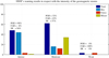 |
Fig. 4. The number of hits, false alarms, and misses for intense, moderate, and weak storm events that occurred in the ascending phases of solar cycles 23 and 24. The total number of storm events in each category is also given for comparison purposes. |
SWIF’s alert criteria are designed to capture storm-associated solar wind disturbances at L1 point. In this respect, seeking possible explanations for SWIF’s failures, i.e., missed events and false alarms, we analyzed the SWIF’s results in respect to the interplanetary causes of the geomagnetic storms. The corresponding information is provided in Tables 2 and 4. As explained previously, only a rough correlation is attempted here to have an indication of the possible limitations. The results are presented in Figure 5, which provides the number of CME-related and non-CME related cases that were received as “True”, “False”, or “Miss” alerts. The results show that the overwhelming majority of hits or true alerts are received under the occurrence of storms related to interplanetary CME signatures. False alarms tend to be related to non-CME structures, while such structures are related also to a significant number of misses.
 |
Fig. 5. The number of CME and non-CME related storm cases for True (hits), False alarms, and Misses in the ascending phases of solar cycle, 23 and 24. |
3.2. Evaluation of SWIF’s performance in capturing storm time disturbances
In this section we investigate the efficiency of the SWIF model in capturing the morphology and the intensity of the ionospheric storm time effects. As a first step, we focus our analysis on the high latitude ionosphere in support of the recent enhancements in the implementation of the model. To this effect, we start by presenting in Figure 6 the SWIF’s output for Tromso with respect to actual observations and ionospheric reference values during two recent storm events that occurred in the time intervals 23–25 April 2012 and 6–8 June 2013. These cases could also be considered indicative examples of the limitations that the limited data availability over high latitude stations may impose in our analysis and results. The problem becomes more pronounced when we work with data of 1 h resolution instead of 15 min time resolution (also visible in Fig. 6), which is a requirement in our case since SWIF’s forecasts are provided with hourly time resolution. Nevertheless, the inspection of all data series obtained in indicative case studies like the ones presented in Figure 6 gives evidence that the SWIF’s predictions follow successfully the general trend of the disturbances during storm days.
 |
Fig. 6. SWIF’s output for Tromso (blue line) in respect to actual observations in hourly (green solid line) and 15 min (green dashed line) time resolution and monthly median estimates (red line) during two recent storm events that occurred in the time intervals 23–25 April 2012 and 6–8 June 2013. The vertical lines note the storm onset in L1 point as it was identified by SWIF ADA. |
To support further our argument, foF2 observations obtained over Tromso during a set of storm events in solar cycle 24 were systematically compared with SWIF’s output. The selection of the storm events considered in this part of the analysis was based on the data availability and the SWIF’s alert results. The list of the events is given in Table 6 and includes cases for which a true alert was received by ADA. In this framework, we present in Figure 7 the distribution of SWIF’s forecasts for the storm days in comparison with the corresponding distribution of actual observations. Here we need to clarify that, although the SWIF’s forecasts are given with hourly resolution, the distribution of the actual observations is based on data of 15 min resolution. One may argue that this discrepancy does not allow the fair comparison of the results, but given the known limitations in the availability of hourly observations as they are discussed above and the bias that these limitations may introduce in the results (see the relevant discussion in Sect. 2), we believe that this approach ensures a more reliable representation of the actual conditions and therefore provides the basis for a rough but indicative evaluation of the trends. Despite the differences detected between the two distributions, their qualitative and quantitative characteristics appear to be very similar verifying SWIF’s efficiency in following the storm time disturbances. Next, we present in Figure 8 the same distributions in a box plot format in comparison with the corresponding output obtained for Chilton during the same storm days. The distributions of the forecasts are displaced to lower than the observed values in both sites indicating same tendency in the accuracy of the model’s predictions in the two latitudinal zones. This may be considered as additional evidence in support of the validity of SWIF’s expansion in high latitudes. Although the limitations in the data availability in Tromso do not allow a comprehensive analysis of the results, one may note that the forecasts increase the distribution width in high latitudes indicating lower precision of the forecasts in this latitudinal zone.
 |
Fig. 7. The distribution of SWIF’s predictions (red bars) for Tromso in respect to the distribution of the actual observations of 15 min resolution (blue bars) during storm days. The mean observed and mean predicted values together with the corresponding STDs are also noted. |
 |
Fig. 8. The distributions of SWIF’s predictions and actual observations over Tromso and Chilton in a box plot format. This includes a box and whisker plot for each case. The box has lines at the lower quartile, median (red line), and upper quartile values. Whiskers extend from each end of the box to the adjacent values in the data; in our case to the most extreme values within 1.5 times the interquartile range from the ends of the box. Outliers (i.e., data with values beyond the ends of the whiskers) are not displayed for visualization purposes. The figure includes also the estimates of the mean observed and mean predicted values and the standard deviations in each case in order to provide a comprehensive statistical overview of the results. |
List of storm events from solar cycle 24 that were analyzed for the evaluation of the SWIF’s performance over Europe.
To quantify the SWIF’s performance during geomagnetic storm conditions several metric parameters were estimated for each of the storm days under consideration. These include: the mean error (ME in MHz) defined as the difference of the modeled from the observed value, the mean relative error (MRE in %) defined as  , the root mean square error (RMSE) in MHz, and the relative improvement over climatology. The latter is calculated by using the following formula:
Relevant results are presented in Table 7. The results were obtained during the storm days in the time intervals listed in Table 6 for three European locations, Tromso, Chilton, and Rome, representative of three latitudinal zones: high, middle-to-high, and middle-to-low, respectively. Nevertheless, since for this part of the analysis we had to work with hourly values due to the limitations in data availability as discussed above, the corresponding results obtained over Tromso may be considered only as indicative of the identified trends.
Metric parameters estimated to quantify SWIF’s performance in solar cycle 24.
The ME values indicate the unbiased performance of the model in all latitudes. The relative improvement over climatology ranges from about 28% at lower latitudes up to 38% at middle-to-high latitudes, demonstrating efficiency of the model to capture about one third of the disturbance’s magnitude in all cases. The averaged MRE is about 20% in all latitudes. No clear dependence on the intensity of the geomagnetic storm was identified in the accuracy of the forecasts.
In order to provide a comprehensive discussion of the results, we performed similar tests of the model’s performance in solar cycle 23. Since such tests have been already carried out for middle latitudes (Tsagouri & Belehaki 2008; Tsagouri et al. 2009; Tsagouri 2011), in this part of the work we concentrate on the high latitude ionosphere. The selection of the test events was once again driven by data availability and SWIF’s alert results. The test events occurred in the ascending phase of solar cycle 23 for direct comparison. The events and the relevant results obtained over Tromso are listed in Table 8 to show that the quantitative characteristics of the model’s performance over Tromso are comparable in the two solar cycles, although the intensity of the geomagnetic storm events is significantly greater in the second case. For further comparisons, one has to take into account the following results reported for the middle latitudes and the previous solar cycle: (i) in a similar investigation Tsagouri & Belehaki (2008) provide evidence of relative improvement over climatology 43% in the middle-to-high latitudes and 30% in the middle-to-low latitudes, (ii) the MRE is found to be around 27% in the middle-to-high latitudes and 22% in the middle-to-low latitudes (Tsagouri & Belehaki 2008; Tsagouri 2011), and (iii) the averaged ME is found to be −0.80 and 0.30 for middle-to-high and middle-to-low latitudes, respectively.
Metric parameters estimated to quantify SWIF’s performance in solar cycle 23.
All relevant results support the following points:
-
Unbiased performance of the forecasts in the two solar cycles.
-
The relative improvement over climatology is quantitatively comparable in the two solar cycles following the same trends: it is estimated to be about 29% in middle-to-low latitudes, 41% in middle-to-high latitudes, and 31% in the high latitudes.
-
Regarding the accuracy, the MRE is about 20% in all latitudes in solar cycle 24. This is also comparable with the results obtained in solar cycle 23 for middle-to-low and high latitudes. However, the MRE for middle-to-high latitudes is higher in the previous solar cycle, reaching the value of 27%. According to previous results, the model tends to underestimate the magnitude of the disturbances, while the prediction error depends on the ionospheric activity level tending to be higher for high ionospheric activity (Tsagouri & Belehaki 2008; Tsagouri 2011).
-
There is no clear dependence of the model’s efficiency in capturing the disturbances on the intensity of the geomagnetic storms.
4. Discussion
To meet DIAS and ESA/SSA/SWE user requirements for HF propagation purposes over Europe, DIAS ionospheric forecasting services were recently expanded to cover whole Europe, including Scandinavia. This was accomplished through enhancements in SWIF’s operational implementation in DIAS system, which was proven to be flexible enough to overcome the restrictions that were imposed due to data availability issues at high latitudes. However, there are two compromises made for the sake of the unbiased and continuous streaming of SWIF’s forecasts in this region: (i) The normal ionospheric variation, which is required for the storm time forecasts, is represented by the CCIR model instead of the running median that is used for middle latitudes, but this is not expected to affect significantly the model’s performance during storm conditions. Preliminary tests that compare CCIR values with reliable monthly median values (i.e., values obtained taking into account at least 17 days in a month) over Tromso in 2013 gave the mean relative deviation equal to 8%. (ii) The non-storm forecasts are also provided by CCIR grids instead of TSAR that runs for middle-latitude forecasts in non-storm conditions. Ideally, the non-storm forecasts should be able to capture both normal and transient ionospheric variation induced by all relevant sources of influence, excluding of course the storm-related variability. However, CCIR predictions are considered representative only for the normal ionospheric variation and, therefore, this second compromise is possible to impose extra limitations in SWIF’s performance at high latitudes during non-storm conditions. Based on the results presented by Tsagouri (2011), the model’s MRE during non-storm conditions (i.e., quiet and moderately disturbed) is estimated to be about 15–17%.
The performance of the SWIF was then extensively evaluated over Europe during storm conditions in the current and the past solar cycle. Concerning the alert detection efficiency, the results verify the exceptionally successful performance of SWIF alert component in predicting the occurrence of ionospheric disturbances associated with intense storm events. For such conditions, the POD reaches 98%, SR 94% while the FAR does not exceed 6%. Nevertheless, the prediction ability of the alert algorithm is poorer in case of ionospheric disturbances that follow the occurrence of moderate storm events. Moderate storm events dominate in the less active solar cycle 24 and this explains the poorer performance of the SWIF model in this solar cycle that was also evident by the evaluation results. The overall performance in the two solar cycles is quantified by 63%, 23%, and 77% for POD, FAR, and SR, respectively, based on the input provided in Tables 3 and 5, while significant limitations in SWIF’s warning ability are attributed to missed events. One has to note that this type of failure is of crucial importance for ionospheric applications, especially under the occurrence of strong negative storm effects and should be the main consideration of future improvements in SWIF’s formulation.
The identified trends are tightly related to the validity of the alert criteria, and therefore, to the efficiency of SWIF’s alert criteria in capturing storm-related interplanetary structures at L1 point. One has to keep in mind that these criteria were extracted through the superposed epoch analysis of intense storm events (occurred in solar cycle 23) that are usually driven by CME-associated solar wind flows at L1 point (e.g., Zhang et al. 2007; Richardson & Cane 2012). Indeed, the results obtained by Echer et al. (2008) that characterized the interplanetary causes of the intense storm events occurring during solar cycle 23 indicate that 87% of the storm events (26 out of 30) included in the development of the model (listed in Table 2 in Tsagouri & Belehaki 2008) were associated with the passage of interplanetary CMEs – mainly magnetic cloud (MC) ones – and/or their associated sheaths. Sheath fields and MC interplanetary CMEs are also the main drivers of most of the intense storm events occurring in solar cycle 23 and all intense storms occurring in solar cycle 24 until November 2012 (Richardson 2013), and they were all correctly forecasted by SWIF. In contrast, Echer et al. (2013) analyzed the interplanetary causes of moderate-intensity geomagnetic storms that occurred in solar cycle 23 (1996–2008) to demonstrate that most of these storms were associated with CIRs and pure HSSs (47.9%), followed by MCs and noncloud ICMEs (20.6%), pure sheath fields (10.8%), and sheath and ICME combined occurrence (9.9%). The HSSs as the dominant driver of moderate storms were also recognized by Richardson & Cane (2012). Taking into account the high warning ability of SWIF alert algorithm under the occurrence of intense storm events and the poorer performance for ionospheric disturbances that follow the occurrence of moderate storm events, it sounds reasonable to conclude that in practice SWIF alert criteria were designed to effectively anticipate the ionospheric storm time effects that occur under specific interplanetary conditions, e.g., cloud ICMEs and/or associated sheaths. In contrast, HSSs and probable CIRs, which are able to drive geomagnetic storms of moderate intensity followed by significant ionospheric disturbances (e.g., Pokhotelov et al. 2010; Tsurutani et al. 2014), are probably not effectively captured by the present criteria. Future analysis of the interplanetary conditions during such events is required to further support the argument and drive a more sophisticated formulation of SWIF’s criteria.
The SWIF was proven able to provide unbiased forecasts in all cases, with comparable performance in the two solar cycles. It offers an improvement over climatology of about 30% in middle-to-low and high latitudes and of a 40% in middle-to-high latitudes. This result indicates that SWIF is able to capture on average more than one third (35%) of the storm-associated ionospheric disturbances. The efficiency of SWIF in capturing the disturbances over Europe was comparatively evaluated (Tsagouri 2011) with the Geomagnetically Correlated Autoregression Model (GCAM; Muhtarov et al. 2002), which also runs in DIAS system and IRI-2000, which includes the STORM model (Araujo-Pradere et al. 2002) as the storm time correction and it is able to capture much of the repeatable characteristics of the storm time ionospheric response. The tests were carried out over the same storm events that occurred in solar cycle 23 in the middle-latitude zone. The results gave evidence of comparable performance between SWIF and GCAM, while the averaged relative improvement over climatology for IRI2000 was estimated to be about 20% and 10% for middle-to-high and middle-to-low latitude, respectively, indicating the successful performance of SWIF in alignment with current ionospheric capabilities in operational mode.
Regarding the accuracy, the averaged MRE is about 20% in middle-to-low and high latitudes, and 24% in the middle-to-high latitudes. However, since the model tends to underestimate the magnitude of the disturbances in all cases, the MRE can reach 30% during very intense negative storms in this latitudinal zone (Tsagouri 2011). In general, the MRE depends on the intensity of the ionospheric activity, tending to be higher for high ionospheric activity. This is expected since the model’s empirical expressions reflect the average ionospheric storm time response, while ionospheric activity greater than 50% is not anticipated by the model. Thus, although no clear dependence of the model’s efficiency in capturing the disturbances on the intensity of the geomagnetic storms was identified for this component of the algorithm, one may expect that improvements in the SWIF’s alert detection capabilities for storms of different interplanetary causes may drive the efforts for a more sophisticated formulation of SWIF’s empirical expressions and therefore of SWIF’s efficiency in capturing the disturbances.
5. Summary and conclusions
This paper discusses recent advances in the implementation and validation of the SWIF model that is running in DIAS to release ionospheric forecasting products for the European region. The upgraded implementation plan expands SWIF’s capabilities in the high latitude ionosphere, including Scandinavia. The SWIF’s products are available through DIAS portal (http://dias.space.noa.gr) and the EIS component of the ESA/SSA/SWE network of services (http://swe.ssa.esa.int/web/guest/dias-federated).
The model’s performance was systematically validated here during the ascending phases of the two solar cycles 23 and 24, complementary to previous validation efforts (e.g., Tsagouri & Belehaki 2008; Tsagouri et al. 2009; Tsagouri 2011). The comprehensive discussion of past and current findings demonstrates that: (i) SWIF’s alert detection algorithm forecasts the occurrence of ionospheric storm time disturbances with probability of detection up to 98% under intense geomagnetic storm conditions and up to 63% when storms of moderate intensity are also considered. The poorer warning ability under the occurrence of weaker storm events is mainly characterized by missed events. (ii) SWIF’s forecasts under successful alerts offer an improvement over climatology of about 30% in middle-to-low and high latitudes and of 40% in middle-to-high latitudes. This indicates that SWIF is able to capture on average more than one third (35%) of the storm-associated ionospheric disturbances. Regarding the accuracy, the averaged MRE during storm conditions usually ranges around 20% in middle-to-low and high latitudes and 24% in the middle-to-high latitudes. The MRE during non-storm conditions (i.e., quiet and moderately disturbed) is estimated about 15–17%.
Our analysis shows that the model’s limitations are related to the efficiency of the alert criteria in capturing storm-related interplanetary structures at L1 point. In particular, the SWIF alert criteria were designed to effectively anticipate the ionospheric storm time effects occurring under specific interplanetary conditions, e.g., magnetic cloud ICMEs and/or associated sheaths. In contrast, HSSs or CIRs seem to be not effectively captured by SWIF’s present formulations. Such interplanetary structures usually drive the development of storm events of moderate intensity (e.g., Richardson & Cane 2012; Echer et al. 2013) that are still able to produce significant ionospheric disturbances as they are described here, but also reported by others (e.g., Pokhotelov et al. 2010; Tsurutani et al. 2014). Such events are often “missed” by SWIF’s ADA. This type of failure is of crucial importance for ionospheric applications, especially under the occurrence of strong negative storm effects and should be the main consideration of future improvements in SWIF’s formulation. A thorough analysis of the interplanetary conditions during such events is expected to make the argument stronger and drive the efforts toward a more sophisticated formulation of the SWIF’s alert criteria.
Acknowledgments
The Dst index is provided by the World Data Center for Geomagnetism, Kyoto (http://wdc.kugi.kyoto-u.ac.jp/dstdir/). This investigation uses historical ionospheric data from Global Ionospheric Radio Observatory (GIRO, http://spase.info/SMWG/Observatory/GIRO). We thank the ACE MAG instrument team and the ACE Science Center for providing the ACE data. SWIF’s alerts and forecasts are offered by DIAS system (http://dias.space.noa.gr) through the real-time Digisonde data streaming from Observatorio del Ebre (Spain), Institute for Atmospheric Physics (Czech Republic), Juliusruh Observing Station, Leibnitz University (Germany), INTA (Spain), RAL Space STFC (UK), IZMIRAN (Russia), INGV (Italy), and NOA (Greece). The upgrade of the SWIF model was performed to improve services delivered to ESA SSA SWE portal. This work was performed in the framework of PROTEAS project within GSRT’s KRIPIS action, funded by Greece and the European Regional Development Fund of the European Union under the O.P. Competitiveness and Entrepreneurship, NSRF 2007–2013 and the Regional Operational Program of Attica.
The editor thanks two anonymous referees for their assistance in evaluating this paper.
References
- Araujo-Pradere, E.A., T.J. Fuller-Rowell, and M.V. Codrescu. STORM: An empirical storm-time ionospheric correction model 1. Model description. Radio Sci., 37, 1070, 2002, DOI: 107010.1029/2001RS002447. [Google Scholar]
- Belehaki, A., Lj. Cander, B. Zolesi, J. Bremer, C. Juren, I. Stanislawska, D. Dialetis, and M. Hatzopoulos. DIAS project: The establishment of a European digital upper atmosphere server. J. Atmos. Sol. Terr. Phys., 67 (12), 1092–1099, 2005. [CrossRef] [Google Scholar]
- Belehaki, A., Lj. Cander, B. Zolesi, J. Bremer, C. Juren, I. Stanislawska, D. Dialetis, and M. Hatzopoulos. Monitoring and forecasting the ionosphere over Europe: The DIAS project. Space Weather, 4, s12002, 2006, DOI: 10.1029/2006SW000270. [Google Scholar]
- Belehaki, A., Lj. Cander, B. Zolesi, J. Bremer, C. Juren, I. Stanislawska, D. Dialetis, and M. Hatzopoulos. Ionospheric specification and forecasting based on observations from European ionosondes participating in DIAS project. Acta Geophys., 55 (3), 398–409, 2007, DOI: 10.2478/s11600-007-0010-x. [NASA ADS] [CrossRef] [Google Scholar]
- Bilitza, D. International Reference Ionosphere 2000. Radio Sci., 36 (2), 261–276, 2001. [CrossRef] [Google Scholar]
- CCIR. Atlas of Ionospheric Characteristics, Comité Consultatif International des Radiocommunications, Report 340-6, International Telecommunications Union, Geneva, 1991. [Google Scholar]
- Echer, E., W.D. Gonzalez, B.T. Tsurutani, and A.L.C. Gonzalez. Interplanetary conditions causing intense geomagnetic storms (Dst ≤ −100 nT) during solar cycle 23 (1996–2006). J. Geophys. Res., 113, A05221, 2008, DOI: 10.1029/2007JA012744. [Google Scholar]
- Echer, E., B.T. Tsurutani, and W.D. Gonzalez. Interplanetary origins of moderate (−100 nT <Dst ≤ −50 nT) geomagnetic storms during solar cycle 23 (1996–2008). J. Geophys. Res., 118, 385–392, 2013, DOI:10.1029/2012JA018086. [Google Scholar]
- Forbes, J.M., S.E. Palo, and X. Zhang. Variability of the ionosphere. J. Atmos. Sol. Terr. Phys., 62, 685–693, 2000. [Google Scholar]
- Gonzalez, W.D., and B.T. Tsurutani. Criteria of interplanetary parameters causing intense magnetic storms (Dst < −100 nT). Planet. Space Sci., 35, 1101–1109, 1987. [Google Scholar]
- Gonzalez, W.D., B.T. Tsurutani, and A.L. Gonzalez. Interplanetary origin of geomagnetic storms. Space Sci. Rev., 88, 529–562, 1999. [Google Scholar]
- Gonzalez, W.D., A.L.C. de Gonzalez, J.H.A. Sobral, A. Dal Lago, and L.E. Vieira. Solar and interplanetary causes of very intense geomagnetic storms. J. Atmos. Sol. Terr. Phys., 63 (5), 403–412, 2001. [CrossRef] [Google Scholar]
- Hunsucker, R.D., and J.K. Hargreaves. The high latitude ionosphere and its effects in radio propagation, Cambridge University Press, Cambridge, UK, ISBN: 0521330831, 2003. [Google Scholar]
- Kazimirovsky, E.S., and V.D. Kokourov. The tropospheric and stratospheric effects in the ionosphere. J. Geomag. Geoelectr., 43 (Suppl.), 551–562, 1991. [CrossRef] [Google Scholar]
- Koutroumbas, K., I. Tsagouri, and A. Belehaki. Time series autoregression technique implemented on-line in DIAS system for ionospheric forecast over Europe. Ann. Geophys., 26, 371–386, 2008. [Google Scholar]
- Lilensten, J., Lj. R. Cander, M.T. Rietveld, P.S. Cannon, and M. Barthelemy. Comparison of EISCAT and ionosonde electron densities: application to a ground-based ionospheric segment of a space weather programme. Ann. Geophys., 23, 183–189, 2005. [CrossRef] [Google Scholar]
- Mendillo, M., H. Rishbeth, R. Roble, E. Damboise, and J. Wroton. Ionospheric variability originating from tropospheric and stratospheric sources. EOS Transactions, 79 (17), 238, 1998. [CrossRef] [Google Scholar]
- Muhtarov, P., I. Kutiev, and L. Cander. Geomagnetically correlated autoregression model for short-term prediction of ionospheric parameters. Inverse Prob., 18, 49–65, 2002. [CrossRef] [Google Scholar]
- Pokhotelov, D., P.T. Jayachandran, C.N. Mitchell, and M.H. Denton. High-latitude ionospheric response to co-rotating interaction region- and coronal mass ejection-driven geomagnetic storms revealed by GPS tomography and ionosondes. Proc. R. Soc. London: Ser. A, 466, 3391–3408, 2010, DOI: 10.1098/rspa.2010.0080. [Google Scholar]
- Prölss, G.W. On explaining the local time variation of ionospheric storm effects. Ann. Geophys., 11, 1–9, 1993. [Google Scholar]
- Richardson, I.G., and H.V. Cane. Near-earth interplanetary coronal mass ejections during solar cycle 23 (1996–2009): Catalog and summary of properties. Sol. Phys., 264 (1), 189–237, 2010. [NASA ADS] [CrossRef] [Google Scholar]
- Richardson, I.G. Geomagnetic activity during the rising phase of solar cycle 24. J. Space Weather Space Clim., 3, A08, 2013. [CrossRef] [EDP Sciences] [Google Scholar]
- Richardson, I.G, and H.V. Cane. Solar wind drivers of geomagnetic storms during more than four solar cycles. J. Space Weather Space Clim., 2, A01, 2012. [Google Scholar]
- Tsagouri, I., A. Belehaki, G. Moraitis, and H. Mavromihalaki. Positive and negative ionospheric disturbances at middle latitudes during geomagnetic storms. Geophys. Res. Lett., 27 (21), 3579–3582, 2000. [Google Scholar]
- Tsagouri, I., and A. Belehaki. A new empirical model of middle latitude ionospheric response for space weather applications. Adv. Space Res., 37, 420–425, 2006. [Google Scholar]
- Tsagouri, I., and A. Belehaki. An upgrade of the solar wind driven empirical model for the middle latitude ionospheric storm time response. J. Atmos. Sol. Terr. Phys., 70 (16), 2061–2076, 2008, DOI: 10.1016/j.jastp.2008.09.010. [Google Scholar]
- Tsagouri, I., K. Koutroumbas, and A. Belehaki. Ionospheric foF2 forecast over Europe based on an autoregressive modeling technique driven by solar wind parameters. Radio Sci., 44, RS0A35, 2009, DOI: 10.1029/2008RS004112. [CrossRef] [Google Scholar]
- Tsagouri, I. Evaluation of the performance of DIAS ionospheric forecasting models. J. Space Weather and Space Clim., 1, A02, 2011, DOI: 10.1051/swsc/2011110003. [Google Scholar]
- Tsurutani, B.T., and W.D. Gonzalez. The future of geomagnetic storm predictions: implications from recent solar and interplanetary observations. J. Atmos. Sol. Terr. Phys., 57, 1369–1384, 1995. [Google Scholar]
- Tsurutani, B., E. Echer, K. Shibata, O. Verkhoglyadova, A. Mannucci, W.D. Gonzalez, U. Janet, J.U. Kozyra, and M. Pätzold. The interplanetary causes of geomagnetic activity during the 7–17 March 2012 interval: a CAWSES II overview. J. Space Weather Space Clim., 4, A02, 2014. [CrossRef] [EDP Sciences] [Google Scholar]
- Zhang, J., I.G. Richardson, D.F. Webb, N. Gopalswamy, E. Huttunen, et al. Solar and interplanetary sources of major geomagnetic storms (Dst ≤ −100 nT) during 1996–2005. J. Geophys. Res., 112, A12105, 2007, DOI: 10.1029/2007JA012332. [CrossRef] [Google Scholar]
- Zolesi, B., Lj. R. Cander, and G. De Franceschi. Simplified ionospheric regional model for telecommunication applications. Radio Sci., 28 (4), 603–612, 1993. [CrossRef] [Google Scholar]
- Zolesi, B., and Lj. R. Cander. The European COST (Co-operation in the field of Scientific and Technical Research) Actions: an important chance to cooperate and to grow for all the international ionospheric community. In: J. Goodman, Proceedings of the 12th International Ionospheric Effects Symposium, 13–15 May 2008, Alexandria, VA, USA, 2008, 110–117 (available from www.ntis.gov, PB2008112709). [Google Scholar]
Cite this article as: Tsagouri I., & A. Belehaki. Ionospheric forecasts for the European region for space weather applications. J. Space Weather Space Clim., 5, A9, 2015, DOI: 10.1051/swsc/2015010.
All Tables
Annual percentage of data availability for four consecutive years over two European stations, Tromso and Chilton.
SWIF’s alert results for the ascending phase of solar cycle 24 (fourth column) in respect to the interplanetary causes of the storms, classified into two categories: CME and non-CME related drivers (fifth column). The corresponding storm time interval is noted in the first column, while the date and time (in UT) that the SWIF alert was received and the min Dst for each storm event are presented in the second and the third column, respectively.
Statistical results of the SWIF alerts performance during solar cycle 24 (ascending phase).
Statistical results of the SWIF alerts performance during solar cycle 23 (ascending phase).
List of storm events from solar cycle 24 that were analyzed for the evaluation of the SWIF’s performance over Europe.
All Figures
|
Fig. 1. The number of days (NoDs), averaged over all months that contribute to the estimation of the monthly median value over Tromso for each hour of day and each year of the analysis. |
| In the text | |
|
Fig. 2. A schematic diagram of the SWIF algorithm for middle and high latitude ionospheric forecasts over Europe. |
| In the text | |
|
Fig. 3. SWIF’s alert response per year during the ascending phases of solar cycles 24 (a) and 23 (b). |
| In the text | |
|
Fig. 4. The number of hits, false alarms, and misses for intense, moderate, and weak storm events that occurred in the ascending phases of solar cycles 23 and 24. The total number of storm events in each category is also given for comparison purposes. |
| In the text | |
|
Fig. 5. The number of CME and non-CME related storm cases for True (hits), False alarms, and Misses in the ascending phases of solar cycle, 23 and 24. |
| In the text | |
|
Fig. 6. SWIF’s output for Tromso (blue line) in respect to actual observations in hourly (green solid line) and 15 min (green dashed line) time resolution and monthly median estimates (red line) during two recent storm events that occurred in the time intervals 23–25 April 2012 and 6–8 June 2013. The vertical lines note the storm onset in L1 point as it was identified by SWIF ADA. |
| In the text | |
|
Fig. 7. The distribution of SWIF’s predictions (red bars) for Tromso in respect to the distribution of the actual observations of 15 min resolution (blue bars) during storm days. The mean observed and mean predicted values together with the corresponding STDs are also noted. |
| In the text | |
|
Fig. 8. The distributions of SWIF’s predictions and actual observations over Tromso and Chilton in a box plot format. This includes a box and whisker plot for each case. The box has lines at the lower quartile, median (red line), and upper quartile values. Whiskers extend from each end of the box to the adjacent values in the data; in our case to the most extreme values within 1.5 times the interquartile range from the ends of the box. Outliers (i.e., data with values beyond the ends of the whiskers) are not displayed for visualization purposes. The figure includes also the estimates of the mean observed and mean predicted values and the standard deviations in each case in order to provide a comprehensive statistical overview of the results. |
| In the text | |
Current usage metrics show cumulative count of Article Views (full-text article views including HTML views, PDF and ePub downloads, according to the available data) and Abstracts Views on Vision4Press platform.
Data correspond to usage on the plateform after 2015. The current usage metrics is available 48-96 hours after online publication and is updated daily on week days.
Initial download of the metrics may take a while.