| Issue |
J. Space Weather Space Clim.
Volume 8, 2018
|
|
|---|---|---|
| Article Number | A41 | |
| Number of page(s) | 14 | |
| DOI | https://doi.org/10.1051/swsc/2018030 | |
| Published online | 03 October 2018 | |
Research Article
The responses of the earth’s magnetopause and bow shock to the IMF Bz and the solar wind dynamic pressure: a parametric study using the AMR-CESE-MHD model
1
Key Laboratory of Earth and Planetary Physics, Institute of Geology and Geophysics, Chinese Academy of Sciences, Beijing, PR China
2
University of Chinese Academy of Sciences, Beijing, PR China
* Corresponding author: This email address is being protected from spambots. You need JavaScript enabled to view it.
Received:
1
February
2018
Accepted:
21
August
2018
Abstract
We have used the AMR-CESE-MHD model to investigate the influences of the IMF Bz and the upstream solar wind dynamic pressure (Dp) on Earth’s magnetopause and bow shock. Our results present that the earthward displacement of the magnetopause increases with the intensity of the IMF Bz. The increase of the northward IMF Bz also brings the magnetopause closer to the Earth even though with a small distance. Our simulation results show that the subsolar bow shock during the southward IMF is much closer to the Earth than during the northward IMF. As the intensity of IMF Bz increases (also the total field strength), the subsolar bow shock moves sunward as the solar wind magnetosonic Mach number decreases. The sunward movement of the subsolar bow shock during southward IMF are much smaller than that during northward IMF, which indicates that the decrease of solar wind magnetosonic Mach number hardly changes the subsolar bow shock location during southward IMF. Our simulations also show that the effects of upstream solar wind dynamic pressure (Dp) changes on both the subsolar magnetopause and bow shock locations are much more significant than those due to the IMF changes, which is consistent with previous studies. However, in our simulations the earthward displacement of the subsolar magnetopause during high solar wind Dp is greater than that predicted by the empirical models.
Key words: magnetopause / bow shock / IMF Bz / solar wind dynamic pressure
© J. Wang et al., Published by EDP Sciences 2018
 This is an Open Access article distributed under the terms of the Creative Commons Attribution License (http://creativecommons.org/licenses/by/4.0), which permits unrestricted use, distribution, and reproduction in any medium, provided the original work is properly cited.
1 Introduction
The interaction between the solar wind and the Earth’s dipole magnetic field forms a magnetic cavity, the outer boundary of which separates most of the solar wind plasma from the region dominated by the Earth’s internal magnetic field, which is named the magnetopause (Chapman and Ferraro, 1930; Willis, 1975). The magnetopause location is physically balanced by the total pressure in the magnetosheath and the magnetic pressure in the magnetosphere. Generally speaking, subsolar point of the magnetopause is located about 10.0 RE from the Earth under normal solar conditions (Spreiter and Stahara, 1985; Shue et al., 1997; De Keyser et al., 2005). When the supersonic and superalfvénic solar wind encounters the magnetospheric obstacle, causing a complex dimpled bow shock structure at the interface between them. The position and shape of the bow shock is physically determined by the incident solar wind conditions and the position and shape of the magnetopause. The subsolar point of the bow shock is generally located about 15.0 RE under normal solar wind conditions (Farris et al., 1991; Cairns and Lyon, 1995; Fairfield et al., 2001; Chapman and Cairns, 2003; Merka et al., 2003).
The shapes, locations, and motions of the Earth’s bow shock and magnetopause have been extensively studied for decades. A number of the previous investigations revealed that the bow shock position and shape are primarily controlled by Dp (Binsack and Vasyliunas, 1968; Formisano, 1979; Farris and Russell, 1994; Chao et al., 2002; Nĕmeček et al., 2016), the upstream Mach numbers (Slavin and Holzer, 1981; Farris and Russell, 1994; Fairfield et al., 2001; Chapman and Cairns, 2003; Verigin et al., 2003), and the orientation and intensity of the interplanetary magnetic field (IMF) (Slavin et al., 1996; Sterck et al., 1998; Kabin, 2001; Chao et al., 2002; Chapman et al., 2004). In addition, the bow shock position and shape are also affected by the magnetopause position and shape that are mainly determined by the solar wind and IMF conditions (Sibeck et al., 1991; Petrinec and Russell, 1993, 1996; Roelof and Sibeck, 1993; Shue et al., 1997, 1998; Kuznetsov and Suvorova, 1998; Chao et al., 2002; Dmitriev et al., 2011; Jelínek et al., 2012).
Based on satellite observations, a large number of empirical models have been established for studying the position and shape of the bow shock (Farris and Russell, 1994; Peredo et al., 1995; Chao et al., 2002; Jeřáb et al., 2005; Merka et al., 2005). Farris and Russell (1994) suggested that the position and shape of the bow shock strongly depends on the position and shape of the magnetopause. In addition, the physical behavior of the bow shock as a function of Dp must be taken into consideration. Some empirical bow shock models assumed the rotational symmetry along the Sun-Earth line (Bennett et al., 1997; Chao et al., 2002). However, some observations reported deviations from rotational symmetry for the bow shock (Peredo et al., 1995). By using a large set of the bow shock crossings, Peredo et al. (1995). confirmed that the north-south extent of the bow shock cross section in the terminator plane is larger than the east-west extent. However, they suggested that the empirical formula may be not adequate to describe the interaction between the solar wind and the magnetosphere. By improving upon the model of Peredo et al. (1995) and Merka et al.(2005) found that the bow shock surfaces has a very correlation with upstream Alfvén Mach number (MA), which indicated that the bow shock surface expands when MA decreases. They also emphasized the importance of the effects of the IMF orientation to the bow shock location. Nevertheless, the results of Jeřáb et al. (2005) showed that the bow shock location is not a function of the IMF orientation or IMF components while depends linearly on the IMF magnitude. There is a need for further researches to better understand the effects of the IMF on the bow shock.
Various empirical models of the magnetopause (Fairfield, 1971; Holzer and Slavin, 1978; Sibeck et al., 1991; Petrinec and Russell, 1993, 1996; Roelof and Sibeck, 1993; Shue et al., 1997; Kuznetsov and Suvorova, 1998; Chao et al., 2002; Lin et al., 2010; Wang et al., 2013) have been established over the past four decades. The solar wind momentum flux appears to be the primary factor controlling the average sizes of the bow shock and magnetopause, and the IMF orientation is a secondary factor (Fairfield, 1971). The magnetopause location is no more variable during periods of high solar wind dynamic pressure than during periods of the low. Especially, the dayside magnetopause is much more sensitive to the southward IMF than the northward IMF (Sibeck et al., 1991). Similarly, other researchers pointed out that the magnetopause erosion effects are stronger under relatively weaker solar wind dynamic pressure during southward IMF, and the subsolar magnetopause is nearly stationary during northward IMF (Shue et al., 1997; Wang et al., 2013). But it is interesting that the dependence of the magnetopause location on the IMF Bz is still under debate.
However, the empirical models are limited by many factors, such as the number of the spacecraft crossings, the crossing positions, the solar wind time delay, and the application scope. Most spacecraft crossings occur relatively close to the Earth’s equatorial plane, which severely restricts the bow shock and magnetopause empirical models around low latitudes. In the empirical models, an additional cause of uncertainty inherent is the treatment of the time delay from the solar wind measurements to the magnetopause crossings (Lin et al., 2010). Some empirical models did not accurately consider this time delay by introducing imponderable deviations (Roelof and Sibeck, 1993; Shue et al., 1997), while in reality the time delay depends on the highly variable upstream solar wind conditions (King and Papitashvili, 2005). The empirical models are also significantly limited by the relatively narrow application scope of the solar wind conditions under which most of the spacecraft crossings occurred, but which may not be suitable for extreme solar wind conditions.
A physics based MHD model can overcome, to some extent, all these disadvantages of the empirical models discussed above, and it has become a valuable and mature tool for analyzing the responses of the bow shock and magnetopause to the solar wind conditions comparatively, even under extreme solar wind conditions. Global MHD models for the interaction of the solar wind with the Earth’s magnetosphere provide an opportunity to quantify the positions and shapes of the Earth’s bow shock and magnetopause. Usadi et al. (1993) predicted that the magnetotail extends with a large cross section and greater north/south than east/west dimensions during southward IMF. A predictive model of the magnetopause was developed using 3D global MHD simulations for different combinations of dynamic pressure and IMF Bz (Elsen and Winglee, 1997). They directly investigated the asymmetries of the magnetopause between the meridian and equatorial planes. Researchers have focused on the high variability of the bow shock’s 3D shape and geometry in response to changes in Alfvénic Mach number MA, solar wind dynamic pressure and IMF orientation, respectively (Chapman and Cairns, 2003; Chapman et al., 2004). However, few of previous studies comprehensively analyze the effects of the solar wind dynamic pressure and IMF Bz on the positions and shapes of the bow shock and magnetopause. Thus, this subject needs to be further discussed in the future.
By using CESE method in general curvilinear coordinates on a six-component grid system with adaptive mesh refinement (AMR) (Feng et al., 2010, 2012, 2014), we have developed a global MHD model (AMR-CESE-MHD) for the magnetosphere which has been tested against other former numerical magnetospheric models through simulating the Earth’s and Saturn’s magnetospheres (Wang et al., 2014, 2015) and presented the global structures and dynamics of the magnetosphere very well, which are consistent with the observations. In this paper, a detailed parametric study is presented which is carried out by using the AMR-CESE-MHD model to investigate the responses of the Earth’s bow shock and magnetopause to the upstream solar wind conditions. We focus on studying the effects of IMF Bz and Dp on the subsolar positions and tail radii of the bow shock and magnetopause, which can further improve our understanding of the interaction between the solar wind and the Earth’s magnetosphere. We first briefly describe the key points of this model. Next, we present the results of each case with different solar wind conditions shown in Table 1. We then compare the results obtained from our model to those obtained from the empirical models. Finally, we discuss in detail about the mechanisms of the responses of the bow shock and magnetopause to the IMF Bz and Dp.
Cases with different solar wind and imf parameters used in the simulations.
2 MHD model
In this section, the model equations used for studying the interaction between the solar wind and the Earth’s magnetosphere are described briefly. As for the details of AMR-CESE-MHD method for numerically solving the model equations, we can refer to Wang et al. (2014, 2015).
2.1 Model equations and grids
As usual, this model is established by using the ideal MHD equations coupled with an ionosphere model for the closure of FACs. The governing equations can be described as below:![Mathematical equation: $$ \frac{\mathrm{\partial }\mathbf{U}}{\mathrm{\partial }t}+[\nabla \cdot (\stackrel{\tilde }{\mathbf{F}}-{\stackrel{\tilde }{\mathbf{F}}}_{\nu }){]}^T=\mathbf{S}, $$](/articles/swsc/full_html/2018/01/swsc180003/swsc180003-eq1.gif) (1)here the state vector, flux tensor, diffusive control terms and Powell source terms are
(1)here the state vector, flux tensor, diffusive control terms and Powell source terms are![Mathematical equation: $$ \mathbf{U}=\left[\begin{array}{l}\rho \\ \rho \mathbf{u}\\ {\mathbf{B}}_1\\ {e}_1\\ \end{array}\right], $$](/articles/swsc/full_html/2018/01/swsc180003/swsc180003-eq2.gif) (2)
(2)
![Mathematical equation: $$ \nabla \cdot \stackrel{\tilde }{\mathbf{F}}={\left[\begin{array}{l}\rho \mathbf{u}\\ \rho \mathbf{uu}+\mathbf{I}\left(p+\frac{1}{2}{{\mathbf{B}}_1}^2+{\mathbf{B}}_1\cdot {\mathbf{B}}_d\right)-{\mathbf{B}}_1{\mathbf{B}}_1-{\mathbf{B}}_1{\mathbf{B}}_d-{\mathbf{B}}_d{\mathbf{B}}_1\\ \mathbf{uB}-\mathbf{Bu}\\ \mathbf{u}\left({e}_1+p+\frac{1}{2}{{\mathbf{B}}_1}^2+{\mathbf{B}}_1\cdot {\mathbf{B}}_d\right)-\left(\mathbf{u}\cdot {\mathbf{B}}_1\right)\mathbf{B}\\ \end{array}\right]}^T, $$](/articles/swsc/full_html/2018/01/swsc180003/swsc180003-eq3.gif) (3)
(3)
![Mathematical equation: $$ \nabla \cdot {\stackrel{\tilde }{\mathbf{F}}}_{\nu }={\left[\begin{array}{l}0\\ 0\\ \mathbf{I}\left(\nu \nabla \cdot {\mathbf{B}}_1\right)\\ 0\\ \end{array}\right]}^T,\enspace \mathbf{S}=-\nabla \cdot {\mathbf{B}}_1\left[\begin{array}{l}0\\ \mathbf{B}\\ \mathbf{u}\\ \mathbf{u}\cdot {\mathbf{B}}_1\\ \end{array}\right] $$](/articles/swsc/full_html/2018/01/swsc180003/swsc180003-eq4.gif) (4)where ρ, u, p, B(≡ B
1 + B
d
) are the mass density, velocity, thermal pressure, magnetic field, I is a unit tensor, the ratio of specific heats γ is taken to be 5/3, and the energy density
(4)where ρ, u, p, B(≡ B
1 + B
d
) are the mass density, velocity, thermal pressure, magnetic field, I is a unit tensor, the ratio of specific heats γ is taken to be 5/3, and the energy density  . Note that the ideal Ohm’s law E + u × B = 0 is used here for the ideal MHD equations.
The Powell source terms −∇ ⋅ B
1(0,B,u,u ⋅ B
1) (Powell et al., 1999) and the diffusive control terms ∇(ν∇ ⋅ B
1) (Feng et al., 2011) have been added to the MHD Equations (1) to deal with the divergence of the magnetic field. Here, following (Feng et al., 2011),  , where Δt is the timestep of each block, Δx, Δy, Δz are grid spacings in Cartesian coordinates.
Our model is especially designed to simulate planets with strong intrinsic magnetic field which solves the deviation of the magnetic field from the intrinsic dipole field, that is, B is split into time-dependent derived part B 1 and time-independent part B d (Tanaka, 1994), where B d corresponds to the Earth’s intrinsic dipole field with a magnitude of 3.2 × 10⁻⁵ T at the equatorial surface.
Equations (1)–(4) are solved by using the AMR-CESE-MHD method on a six-component grid system based on previously presented numerical algorithms (Feng et al., 2007, 2010; Wang et al., 2014). In the magnetosphere part, the MHD equations are solved as an initial-boundary-value problem in the region from 3.0 to 156.0 RE, while the region within 3.0 RE is treated as a magnetosphere-ionosphere coupling problem. The grid size varies from 0.1 RE near the inner boundary (r = 3.0 RE) to be 3.8 RE near the outer boundary r = 156.0 RE (Wang et al., 2015). The grids have been specially refined by using the adaptive mesh refinement method near the subsolar bow shock and magnetopause where the grid resolutions are 0.2 RE and 0.12 RE respectively.
To show the validity and capability of the AMR-CESE-MHD model, a suite of numerical tests, such as the blast wave problem and MHD vortex problem, in two and three dimensions including ideal MHD and resistive MHD were carried out by Jiang et al. (2010). The results indicated that the CESE MHD solver can handle all these problems very well.
2.2 Magnetosphere-ionosphere coupling
According to Raeder et al. (1998), the coupling between the magnetosphere and ionosphere is established by mapping the field-aligned currents from the magnetosphere to the ionosphere. The ionosphere is treated as a two-dimensional spherical shell at 1.017 RE. Thus a potential equation as below is then solved (Raeder, 2003): (5)where Φ is the ionospheric potential,
  is the intensity of the field-aligned currents and I is the dipole magnetic field inclination angle. Σ denotes the tensor of the ionospheric conductances written as
 (6)where
 (7)where ΣP is the Pedersen conductance and ΣH is the Hall conductance. In Equations (5) and (6), it is assumed that the parallel conductivity is infinite as compared to Equation (1) of Amm and Goodman (1996).
We take the Pedersen conductance to be 5 S and uniform at the northern and southern hemispheres, and neglect the Hall conductance for simplicity. In accordance with Hu et al. (2005), Equation (5) can be reduced to (8)where
It is assumed that the magnetic field is dipole and equipotential in the region between the magnetospheric inner boundary and the ionosphere in this present model. Meanwhile, we neglect the perpendicular currents in order to get the field-aligned currents. According to the current continuity, it follows that J||/B = const along the magnetic field lines in this region from which the field-aligned currents for Equation (5) can be written as  , where
  and
and  denote the field-aligned currents at the ionosphere and the magnetospheric inner boundary respectively, σ is the ratio of the magnetic field strength at the ionosphere and the inner boundary (Merkin and Lyon, 2010).
We take the assumption that the ionospheric potential is a constant at or near the low-latitude boundary of the computational domain. The computational domain of Equation (5) is (0 ≤ θ < 32°) ∩ (0 ≤ φ ≤ 180°), with Δθ = 1° and Δφ = 180°/64. With the conductances and the mapped field-aligned currents at the ionosphere, we solve Equation (5) by using the Newton iteration method. Then, the ionospheric potential is mapped along the magnetic field lines back to the inner boundary (Gombosi et al., 1998), where it is used as the boundary condition for the magnetospheric flow and field by taking  , here the subscript “t”‘ refers to the tangential components of the velocity at the inner boundary. The ionospheric and magnetospheric solutions are coupled together after every time step during the simulations.
2.3 Initial and boundary conditions
Table 1 lists the input parameters of all these cases used in our parametric study, with vysw = 0, vzsw = 0, Bxsw = 0, Bysw = 0, psw = 0.032 nPa in all cases, where the x-axis points from the Earth to the Sun, the z-axis is positive to the north pole and is in the plane which contains the x-axis and the Earth’s dipole axis, and the y-axis completes the right-handed coordinate system. This is the GSM coordinate system. We choose to use very high values of IMF Bz and Dp (the observations under such conditions are very limited) to further study the interaction between the solar wind and the Earth’s magnetosphere. Cases 1, 2, 3 are northward IMF cases, and Cases 4, 5, 6 are southward IMF cases. Case 1 and Case 4 are the classical steady solar wind conditions which are used as the reference cases here. Comparing to Case 1 (or Case 4), Case 2 (or Case 5) has a doubled IMF Bz, and Case 3 (or Case 6) has an increased solar wind dynamic pressure Dp. In this study, we just took into account of the influences of the upstream solar wind dynamic pressure Dp, and not considered the effects of solar wind velocity and density separately. We will conduct a further research on the influences of solar wind velocity and density separately to the locations of the magnetopause and bow shock in our future work.
The sunward side of the plane at x = 15.0 RE is initialized by the solar wind parameters. For the earthward side, the magnetic field is initialized by the superposition of dipole magnetic field and mirror dipole magnetic field to create B x = 0 at the plane of x = 15.0 RE (Raeder, 2003). The density and plasma pressure are initialized according to Ogino (1986). At the dayside of the outer boundary, fixed inflow boundary conditions are applied. At the nightside of the outer boundary, free flow boundary conditions are used. At the inner boundary, the density and pressure are set to fixed values, the radial component of velocity is set to zero, and the tangential component of velocity is determined by the coupling between the inner magnetosphere and the ionosphere as discussed above. In accordance with Song et al. (1999), the tangential components of the time-dependent derived part of magnetic field B 1 are determined by Neumann condition and and its normal component is determined by Dirichlet condition.
3 Simulation results
In this section, we present the simulation results of all these cases listed in Table 1 to study the responses of the bow shock and magnetopause to IMF Bz and Dp. Figures 2–7a show the color contours of the current density ( , in unit: 10−3 μA/m2) in the noon-midnight meridian plane, in which the black lines are the magnetic field lines, and the arrows indicate the magnetic field directions. Figures 2–7b show an illustration of the color contours of the current density in the cross section at x = −20.0 RE. Three current systems can be clearly seen: bow shock current, magnetopause current and cross-tail current, respectively. Closure currents flowing on the magnetopause and the cross tail current form a closed current system which presents a θ-shaped configuration in the cross section. The current intensity of the closed system is much stronger than that around it.
In this paper, we identify the magnetopause and bow shock mainly based on the peaks of the current density, except that the dayside magnetopause positions are defined by the last closed magnetic field lines and the equatorial magnetopause are determined by the flow streamlines.
The presented results have converged with respect to the grid resolutions. The highest resolutions near the subsolar bow shock and magnetopause here are 0.2 RE and 0.12 RE, respectively. Such grid resolutions are enough for this study. Figure 1 presents the convergence behavior of the AMR-CESE-MHD model.
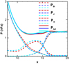 |
Fig. 1. Convergence of the AMR-CESE-MHD model respect to the grid resolutions. The red, blue and light blue lines denote the pressure profiles (P th: thermal pressure, P d: dynamic pressure, P m: magnetic pressure, P tot: total pressure) of Case 1 along Sun-Earth line when the interest regions are refined with first-level, second-level and third-level grids, respectively. |
3.1 Northward IMF cases
For northward IMF, magnetic reconnection takes place near the nightside of the cusp regions between the IMF and the magnetospheric magnetic field. From the magnetic field lines in Figures 2–4a, we find that the magnetosphere is nearly closed unless at the cusp regions. As shown in Figure 2a, the magnetotail could extend to 50.0 RE in Case 1. At the dayside, most of the current forms at the bow shock, and the dayside magnetopause current turns up near the first closed magnetic field line. The nightside magnetopause current peaks (with bright red color) near the cusp regions, extends to the high latitudes and be farther away from the Earth along the magnetic field lines. The distributions of the nightside magnetopause current are almost consistent with locations of the last closed magnetic field lines.
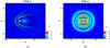 |
Fig. 2. Color contours of the current density (in unit: 10−3 μA/m2) in (a) the meridian plane and (b) the cross section at x = −20.0 R E in the tail for Case 1. Black lines with arrows in the left panel are magnetic field lines. |
Figure 3a presents the color contours of the current density in Case 2, and the magnetotail shrinks remarkably to be about 25.0 RE, nearly half of that in Case 1. Tables 4 and 5 present the subsolar positions and tail radii of the bow shock and magnetopause for each case respectively. It is shown that the subsolar bow shock moves sunward to be further away from the Earth while the subsolar magnetopause moves earthward to be closer to the Earth. The bow shock expands outward while the magnetopause shrinks along both the east-west and north-south directions in the YZ cross section at x = −20.0 RE.
Figure 4a presents that the dayside bow shock and magnetopause are obviously compressed with increasing Dp in Case 3. The flanks of the magnetotail are compressed substantially by the upstream solar wind. The global structure of the magnetosphere remains closed with the magnetotail extending to be more than 100.0 RE. Figure 4b shows that the size of the θ-shaped current system is much smaller than that of Case 1. As shown by Tables 4 and 5, both of the subsolar bow shock and magnetopause move to be closer to the Earth, and both of the nightside bow shock and magnetopause shrink remarkably along east-west and north-south directions in the YZ cross section at x = −20.0 RE as Dp increases.
For northern IMF cases, as shown in Figures 2–4a, we have represented the magnetospheric configurations which are consistent with those in Gombosi et al. (1998) in large scale very well, and we credit this previous work very much.
3.2 Southward IMF cases
The global structure of the magnetosphere for due southward IMF has been widely studied previously. Under due southward IMF, the magnetic reconnection takes place near x = 10.0 RE at the subsolar magnetopause, where the orientations of the IMF and the magnetospheric magnetic field are opposite. The dayside closed magnetospheric magnetic field lines are opened and transported to the magnetotail by the tailward flowing solar wind. The solar wind plasma can enter into the magnetosphere along those open field lines connecting to the high latitude polar regions (Walker et al., 1995). Moreover, magnetic reconnection could take place at the magnetotail current sheet at about x = −10.0 ~ −20.0 RE between the open field lines in the north and south lobes, which can re-close the open tail lobe field lines. The magnetic field lines in Figures 5–7a indicate that for due southward IMF the magnetic field lines in the high latitude are nearly opened and extend to the solar wind while the field lines in the low latitude are closed. Figures 5–7b also reveal three major current systems in the magnetosphere. For due southward IMF, the magnetopause current and the cross tail current could also form a θ-shaped closed system in the YZ cross section.
Figure 6a presents the color contour of the current density with the magnetic field lines in Case 5. The magnetopause current and cross-tail current form a θ-shaped closed system, but the size of which is only a little larger than that of Case 4 as shown by Figure 6b. Table 4 shows that the subsolar bow shock moves to be further away from the Earth. However, the subsolar magnetopause shrinks to be closer to the Earth as shown by Table 5. Moreover, we find that both of the nightside bow shock and magnetopause expand outward along the east-west and north-south directions in the YZ cross section at x = −20.0 RE.
Figure 7a displays the color contour of the current density with the magnetic field lines in Case 6. We can clearly find that the dayside bow shock and magnetopause are compressed by the solar wind to be much closer to the Earth. Figure 7b presents the θs-shaped closed system formed by the magnetopause current and the cross-tail current, the size of which is obviously much smaller than that of Case 4. Tables 4 and 5 show that both of the subsolar bow shock and magnetopause in Case 6 move earthward remarkably, and both of the nightside bow shock and magnetopause shrink severely along east-west and north-south directions in the YZ cross section at x = −20.0 RE, as compared to Case 4.
In accordance to De Zeeuw et al. (2004), the kinetic physics of the inner magnetosphere have substantial effects on the inner magnetospheric pressure. In order to estimate how would the subsolar magnetopause change when the kinetic effects of the inner magnetosphere are included, we have run all these cases by using the BATS-R-US model and the BATS-R-US+CRCM (an inner magnetosphere model) coupled model, and the results of which are compared with those of the AMR+CESE+MHD model as shown by Table 2. The results of the AMR+CESE+MHD model are consistent with those obtained from the BATS-R-US and BATS-R-US+CRCM models very well. The results also show that the subsolar magnetopause moves sunward, with addition of the kinetic physics of the inner magnetosphere (BATS-R-US+CRCM compares with BATS-R-US). However, its influence on the location of subsolar magnetopause is not as great as expected. Although the CRCM model has been added into the simulations, the responses of the subsolar magnetopause to changes of the IMF Bz and the solar wind dynamic pressure are still consistent with our conclusions.
Subsolar magnetopause locations resulted from different models.
4 Comparisons with empirical models
In this section, we try to compare the MHD results with those of the empirical models available for the bow shock (Chao et al., 2002) and magnetopause (Shue et al., 1997), qualitatively. Chao et al. (2002) presented a function to describe the position and shape of the bow shock: (9)where r is the radial distance at a zenith angle (θ) between the direction of r and the positive direction of x-axis, and α controls the level of the tail flaring of the bow shock. The parameter r0 is the bow shock subsolar standoff distance. The best-fit results for the parameters r0, α can be expressed as the functions of Bz, Dp, β and Mms below:
\\ \\ {r}_0={a}_1\left(1+{a}_3{B}_{\mathrm{z}}\right)\left(1+{a}_9\beta \right)\left(1+{a}_4\frac{\left({a}_8-1\right){M}_{\mathrm{ms}}^2+2}{\left({a}_8+1\right){M}_{\mathrm{ms}}^2}\right){D}_p^{-\frac{1}{{a}_{11}}}\enspace \mathrm{for}\enspace {B}_{\mathrm{z}}<0\\ \\ \alpha ={a}_5(1+{a}_6{B}_{\mathrm{z}})(1+{a}_7{D}_{\mathrm{p}})[1+{a}_{10}\mathrm{ln}(1+\beta )](1+{a}_{14}{M}_{\mathrm{ms}})\\ \end{array} $$](/articles/swsc/full_html/2018/01/swsc180003/swsc180003-eq21.gif) (10)where the coefficients are listed in Table 3, and ε in Equation (9) is equal to a12.
(10)where the coefficients are listed in Table 3, and ε in Equation (9) is equal to a12.
Shue et al. (1997) presented a function to fit the position and shape of the magnetopause: where r is the radial distance at a zenith angle (θ) between the direction of r and the positive direction of x-axis, and α controls the level of the tail flaring of the magnetopause. The parameter r0 is the magnetopause subsolar standoff distance. They showed that the best fitting result of r0 and α runs as follows:
 (11)with the coefficients a1 = 11.4, a2 = 0.013, a3 = 0.14, a4 = 6.6, a5 = 0.58, a6 = −0.01, a7 = 0.01.
We get the corresponding values of the subsolar positions and tail radii of the bow shock and magnetopause for each case, which are listed in Tables 4 and 5.  and
and  are get from the bow shock model of Chao et al. (2002), and
  and
and  are established according to the magnetopause model of Shue et al. (1997). The corresponding parameters marked by a superscript star are obtained from our MHD model.
  and
and  are the positions of the subsolar bow shock and magnetopause, respectively. Axial symmetry has been assumed in these two models. Therefore, the cross sections of the bow shock and magnetopause obtained from them are circular. Here,
  and
and  are used to indicate the tail radii of the bow shock and magnetopause at x = −20.0 RE, respectively. Actually, the cross sections of the bow shock and magnetopause are almost elliptical. In Tables 4 and 5, we give out the tail radii of the bow shock and magnetopause along y-axis and z-axis at x = −20.0 RE in our model, which are represented by
  ,
,  ,
,  , and
, and  , respectively.
The bow shock subsolar position and tail radii for each case.
The magnetopause subsolar position and tail radii for each case.
Table 4 shows that, for the northward cases,  and
and  are almost consistent with
  and
and  . However, for the southward cases, the deviations between them are a little greater. The reason for this maybe that few pure southward IMF observations can be obtained in reality which may bring about deviations into the empirical models. Nevertheless, we just intend to compare the responses of the bow shock locations to the IMF Bz and Dp qualitatively in this paper. From Table 4, we find that for the northward cases, both the subsolar position and tail radius at x = −20.0 RE of the bow shock increase remarkably as |Bz| increases. For the southward cases, the nightside bow shock tail radii at x = −20.0 RE increase substantially, while the subsolar position increases with a small scale. Moreover, both the subsolar position and tail radius at x = −20.0 RE of the bow shock decrease remarkably as the solar wind dynamic pressure Dp increases for due northward and southward IMFs.
Table 5 presents that, for both northward and southward cases,  and
and  are nearly consistent with
  and
and  , and the deviations between them are no larger than 1.5 RE. We find that the subsolar position of the magnetopause decreases slightly, and the magnetopause tail radius at x = −20.0 RE decreases as |Bz| increases under northward IMF. For southward IMF, as |Bz| increases, the magnetopause subsolar position decreases slightly, and the magnetopause tail radius increases. Moreover, we find an inverse correlation between the magnetopause subsolar position (or tail radius at x = −20.0 RE) and the solar wind dynamic pressure Dp for both due northward and southward IMFs. Both the subsolar position and the tail radius at x = −20.0 RE of the magnetopause decrease obviously as the solar wind dynamic pressure Dp increases.
Overall, the responses of the bow shock and magnetopause to IMF Bz and Dp from our MHD simulation results described in the above sections are consistent with the empirical models.
5 Discussion
We compare Case 1 and Case 2 to investigate the responses of the subsolar magnetopause and bow shock to the northward IMF Bz. Case 1 and Case 2 have the same upstream solar wind dynamic pressure (Dp), while the IMF Bz intensity in Case 2 is doubled. Figure 8 shows the profiles of the thermal, magnetic, dynamic and total pressures at the Sun-Earth line obtained by the global AMR-CESE-MHD model for Case 1, Case 2 and Case 3. It is clearly seen that the magnetic pressure (Pm) increases obviously along the earthward direction (negative x), the thermal pressure (Pth) increases first and then decreases. Pm becomes the major pressure gradually, and the dynamic pressure (Pd) is nearly zero at the subsolar magnetopause. As the northward IMF Bz increases (see Case 2), more magnetic flux would pile up in the magnetosheath and drape around the magnetopause. Therefore, Pm increases significantly at the dayside magnetopause, and the total pressure (Pt) is larger in Case 2 than that in Case 1 as shown by Figure 8b. Thus, the subsolar magnetopause is compressed and moves earthward (with a displacement ~0.3 RE). A number of studies have shown that the bow shock depends on the upstream solar wind Mach numbers, and the bow shock will move away from the Earth in response to a decrease of the magnetosonic Mach number ( , Mms is the magnetosonic Mach number, vsw is the solar wind speed, and vms is the magnetosonic speed) (Farris and Russell, 1994; Chapman and Cairns, 2003). As usual, the solar wind magnetosonic speed is defined by
  , where cs and vA are the sonic speed and Alfvénic speed respectively. The increase of the intensity of IMF Bz could results in the increase of the Alfvénic speed, and the solar wind vms increases as well. As a result, the solar wind Mms decreases. In response to the decrease of the upstream solar wind Mms, the subsolar bow shock in Case 2 moves outward with a large displacement (~1.4 RE) as shown by Figure 8b.
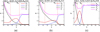 |
Fig. 8. Thermal (Red), magnetic (black), dynamic (blue) and total (pink) pressures (nPa) at the Sun-Earth line obtained by the global AMR-CESE-MHD model for (a) Case 1, (b) Case 2 and (c) Case 3. The red dashed lines denote the subsolar magnetopause locations (R mg) which are defined by the last closed magnetic field lines and the red dash-dotted lines denote the subsolar bow shock locations (R bs) which are determined by the peaks of the current density in our simulations. |
Case 3 is compared with Case 1 to investigate the effects of the upstream solar wind dynamic pressure to the subsolar positions of the magnetopause and bow shock for northward IMFs. These two cases have the same IMF Bz. But the upstream solar wind dynamic pressure and Mms in Case 3 are larger as compared to Case 1. Figure 8c present that Pth and Pd in the magentoheath in Case 3 becomes much greater than that in Case 1. Pt at the subsolar magnetopause increases greatly, so that the dayside magnetopause is compressed severely with a displacement (~2.4 RE) which is a little larger than that predicted by the empirical model (~2.3 RE). As the size of the obstacle (the magnetopause) become much smaller and the upstream solar wind Mms increases, the subsolar bow shock becomes much closer to the Earth with a quite large distance (~4.4 RE).
We also compare the southward cases to study the effects of the IMF Bz and Dp to the subsolar positions of the magnetopause and bow shock under southward IMFs. We find that, as the southward Bz increases, more closed field lines are opened during the dayside magnetic reconnection process, thus the subsolar magnetopause moves earthward with a displacement (~0.6 RE). However, as the solar wind Mms decrease in Case 5, the bow shock move sunward with only a small-scale displacement as compared to Case 4 (see Fig. 9b). It is possible that the position and shape of the magnetopause may also determine the position of the subsolar bow shock in this situation. As shown by Figure 9c, when the solar wind dynamic pressure increases for southward IMF, we find that the magnetopause is compressed remarkably with a displacement (~2.9 RE) which is larger than that predicted by the empirical model (~2.0 RE). It indicates that the dependence of the positions of the subsolar magnetopause on the solar wind dynamic pressure is larger than that predicted by the empirical models. Moreover, the subsolar bow shock is compressed to be much closer to the Earth with a large distance (~4.1 RE) in Case 6. It presents that the solar wind dynamic pressure also dominates the positions of the subsolar magnetopause and bow shock for southward IMFs.
Case 1 and Case 4 are compared to study the effects of the IMF Bz orientations to the locations of the subsolar magnetopause and bow shock. Both of the intensity of IMF Bz and the solar wind Dp are equal in these two cases, but the IMF Bz orientations are opposite. That means the solar wind Mms are equal in these two cases. Under southward IMF, the magnetic reconnection takes place near the subsolar magnetopause where the magnetic flux would be transported from the dayside to the nightside. However, due to the strong intensity of the Earth’s dipole magnetic field, the subsolar magnetopause could moves earthward with only a small distance ~0.3 RE in Case 4 as compared to Case 1. Figure 10 clearly shows that the position and shape of the magnetopause on the equatorial and meridian planes have great changes in Case 4 as compared to Case 1 which means that the subsolar magnetic reconnection have a great effect on the position and shape of the magnetopause. In response to the changes of the position and shape of the magnetopause, the position and shape of the bow shock also have a great change (see Fig. 10). The subsolar bow shock moves earthward and the flaring angle becomes larger. Although the Mms are equal in these two cases, the bow shock still moves earthward in Case 4 as compared to Case 1 which suggests that the position of the bow shock is not only determined by the solar wind Mms, but also determined by the IMF Bz orientations.
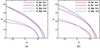 |
Fig. 10. Positions of the magnetopause and bow shock on the (a) equatorial and (b) meridian planes for Case 1 and Case 4 from our simulations. Red solid and dashed lines denote the positions of the bow shock and magnetopause for Case 1, respectively. Blue solid and dashed lines denote the positions of the bow shock and magnetopause for Case 4, respectively. |
As the northward IMF Bz increases, the magnetic reconnection at the cusp regions increases. More closed magnetospheric magnetic field lines rooted on the nightside polar regions are peeled off and accumulate behind the magnetotail, causing the shrinkage of the magnetotail radii and the contraction of the magnetotail. Under due southward IMF, magnetic reconnection takes place at the subsolar magnetopause. As the southward IMF Bz increases, the rate of the dayside magnetic reconnection increases (Lockwood and Wild, 1993). More closed magnetospheric magnetic field lines near the subsolar magnetopause are opened during the dayside magnetic reconnection process, and the tailward solar wind flow bring the magnetic flux from the dayside to the nightside (Shue et al., 1997). The subsolar magnetopause shrinks to be a little closer to the Earth, while the night magnetopause could expand towards the north-south and east-west directions. The magnetopause is primarily determined by the balance between the total pressure of the external solar wind and the magnetosphere. When the solar wind dynamic pressure is increased, for no matter northward IMF or southward IMF, the whole magnetopause can be compressed significantly. We can see that the subsolar magnetopause moves earthward, and the nightside magnetopause shrinks along the north-south and east-west directions. As the size of the obstacle (the magnetopause) becomes much smaller, the whole bow shock moves inside with quite a large distance.
Furthermore, we have also carried out additional runs to study the effects of the IMF Bx and By components to the positions of the subsolar magnetopause and bow shock. Our results show that the dependence of the positions of subsolar magnetopause and bow shock on the IMF Bx and By is rather little. The IMF Bx and By may introduce asymmetry into the shapes of the magnetopause and bow shock.
6 Conclusions
A parametric study is carried out with different values of the IMF Bz and Dp under northward and southward IMFs by using the AMR-CESE-MHD model. Our results present that the increase of the southward IMF Bz could result in an earthward movement of the magnetopause, and the displacement could increase with the intensity of the IMF Bz. The increase of the northward IMF Bz could also bring the magnetopause to move earthward but with a small distance. The subsolar bow shock during southward IMF is much closer to the Earth than during northward IMF. However, as the intensity of IMF Bz increases, the variations of the sunward movement of the subsolar bow shock during southward IMF are much smaller than that during northward IMF, which means that the changes of the subsolar bow shock location with upstream solar wind magnetosonic Mach number are much smaller during southward IMF. We suggest that the orientation of the IMF Bz has an important effect on the subsolar bow shock location. Our simulations also show that the effects of upstream solar wind dynamic pressure (Dp) changes on both the subsolar magnetopause and bow shock locations are much more significant than those due to the IMF changes, which is consistent with previous studies (Farris and Russell, 1994; Shue et al., 1998; Boardsen et al., 2000; Chao et al., 2002). However, in our simulations the earthward displacement of the subsolar magnetopause during high solar wind Dp is greater than that predicted by the empirical models.
Acknowledgments
The work was jointly supported by the National Natural Science Foundation of China (Grant Nos. 41604144, 41531073, 41474144, 41774176), National Key Research and Development Program of China (2016YFB0501300 and 2016YFB0501304) and the Specialized Research Fund for State Key Laboratories. All these simulations were carried out on the computational facilities in the Computer Simulation Lab of IGGCAS. You may obtain the data in this paper by contacting Juan Wang at This email address is being protected from spambots. You need JavaScript enabled to view it. . The editor thanks Ilja Honkonen and an anonymous referee for their assistance in evaluating this paper.
References
- Amm O, Goodman ML. 1996. Comment on: A three-dimensional, iterative mapping procedure for the implementation of an ionosphere-magnetosphere anisotropic Ohm's law boundary condition in global magnetohydrodynamic simulations. Author’s reply. Ann Geophys 14: 773–775. [Google Scholar]
- Bennett L, Kivelson MG, Khurana KK, Frank LA, Paterson WR. 1997. A model of the Earth’s distant bow shock. J Geophys Res 102: 26927–26941. DOI: 10.1029/97JA01906. [CrossRef] [Google Scholar]
- Binsack JH, Vasyliunas VM. 1968. Simultaneous IMP 2 and OGO 1 observations of bow shock compression. J Geophys Res 73: 429–433. DOI: 10.1029/JA073i001p00429. [CrossRef] [Google Scholar]
- Boardsen SA, Eastman TE, Sotirelis T, Green JL. 2000. An empirical model of the high-latitude magnetopause. J Geophys Res 105: 23193–23219. DOI: 10.1029/1998JA000143. [CrossRef] [Google Scholar]
- Cairns IH, Lyon J. 1995. MHD simulations of Earth’s bow shock at low Mach numbers: Standoff distances. J Geophys Res 100: 17173–17180. DOI: 10.1029/95JA00993. [CrossRef] [Google Scholar]
- Chao JK, Wu DJ, Lin CH, Yang YH, Wang XY, Kessel M, Chen SH, Lepping RP. 2002. Models for the size and shape of the Earth’s magnetopause and bow shock. Cospar Colloquia series 12: 127–135. [CrossRef] [Google Scholar]
- Chapman JF, Cairns IH, Lyon JG, Boshuizen CR. 2004. MHD simulations of Earth’s bow shock: Interplanetary magnetic field orientation effects on shape and position. J Geophys Res 109: 215. DOI: 10.1029/2003JA010235. [Google Scholar]
- Chapman JF, Cairns IH. 2003. Three-dimensional modeling of Earth’s bow shock: Shock shape as a function of Alfvén Mach number. J Geophys Res 108: A051174. DOI: 10.1029/2002JA009569. [Google Scholar]
- Chapman S, Ferraro VC. 1930. A new theory of magnetic storms. Nature 126: 129–130. DOI: 10.1038/126129a0. [NASA ADS] [CrossRef] [Google Scholar]
- De Keyser J, Dunlop MW, Owen CJ, Sonnerup BUÖ, Haaland SE, Vaivads A, Paschmann G, Lundin R, Rezeau L. 2005. Magnetopause and boundary layer. Outer magnetospheric boundaries: Cluster results. Space Sci Rev 118: 231–320. DOI: 10.1007/1-4020-4582-4_9. [CrossRef] [Google Scholar]
- De Zeeuw DL, Sazykin S, Wolf RA, Gombosi TI, Ridley AJ, Toth G. 2004. Coupling of a global MHD code and an inner magnetospheric model: Initial results. 109. DOI: 10.1029/2003JA010366. [Google Scholar]
- Dmitriev A, Suvorova A, Chao JK. 2011. A predictive model of geosynchronous magnetopause crossings. J Geophys Res 116. DOI: 10.1029/2010JA016208. [CrossRef] [Google Scholar]
- Elsen RK, Winglee RM. 1997. The average shape of the magnetopause: A comparison of three-dimensional global MHD and empirical models. J Geophys Res 102: 4799–4819. DOI: 10.1029/96JA03518. [CrossRef] [Google Scholar]
- Fairfield DH, Iver HC, Desch MD, Szabo A, Lazarus AJ, Aellig MR. 2001. The location of low Mach number bow shocks at Earth. J Geophys Res 106: 25361–25376. DOI: 10.1029/2000JA000252. [Google Scholar]
- Fairfield DH. 1971. Average and unusual locations of the Earth’s magnetopause and bow shock. J Geophys Res 76: 6700–6716. DOI: 10.1029/JA076i028p06700. [CrossRef] [Google Scholar]
- Farris MH, Russell CT. 1994. Determining the standoff distance of the bow shock: Mach number dependence and use of models. J Geophys Res 99: 17681. DOI: 10.1029/94JA01020. [Google Scholar]
- Farris MH, Petrinec SM, Russell CT. 1991. The thickness of the magnetosheath: Constraints on the polytropic index. Geophys Res Lett 18: 1821–1824. DOI: 10.1029/91GL02090. [Google Scholar]
- Feng XS, Zhou YF, Wu ST. 2007. A novel numerical implementation for solar wind modeling by the modified conservation element/solution element method. Astrophys J 655: 1110. [CrossRef] [Google Scholar]
- Feng XS, Yang LP, Xiang CQ, Wu ST, Zhou YF, Zhong DK. 2010. Three-dimensional solar wind modeling from the Sun to Earth by a SIP-CESE MHD model with a six-component grid. Astrophys J 723: 300. [NASA ADS] [CrossRef] [Google Scholar]
- Feng XS, Zhang S, Xiang CQ, Yang LP, Jiang CW, Wu ST. 2011. A hybrid solar wind model of the CESE+HLL method with a Yin-Yang overset grid and an AMR grid. Astrophys J 734: 50. [Google Scholar]
- Feng XS, Yang LP, Xiang CQ, Jiang CW, Ma XP, Wu ST, Zhong DK, Zhou YF. 2012. Validation of the 3D AMR SIP–CESE solar wind model for four carrington rotations. Solar Phys 279: 207–229. [Google Scholar]
- Feng XS, Xiang CQ, Zhong DK, Zhou YF, Yang LP, Ma XP. 2014. SIP-CESE MHD model of solar wind with adaptive mesh refinement of hexahedral meshes. Comput Phys Comm 185: 1965–1980. DOI: 10.1016/j.cpc.2014.03.027. [CrossRef] [Google Scholar]
- Formisano V. 1979. Orientation and shape of the Earth’s bow shock in three dimensions. Planet Space Sci 27: 1151–1161. DOI: 10.1016/0032-0633(79)90135-1. [CrossRef] [Google Scholar]
- Gombosi TI, DeZeeuw DL, Groth CPT, Powell KG, Song P. 1998. The length of the magnetotail for northward IMF: Results of 3D MHD simulations. Phys Space Plasmas 15: 121–128. [Google Scholar]
- Holzer RE, Slavin JA. 1978. Magnetic flux transfer associated with expansions and contractions of the dayside magnetosphere. J Geophys Res 83: 3831–3839. DOI: 10.1029/JA083iA08p03831. [CrossRef] [Google Scholar]
- Hu YQ, Guo XC, Li GQ, Wang C, Huang ZH. 2005. Oscillation of quasi-steady Earth’s magnetosphere. Chin Phys Lett 22: 2723. [CrossRef] [Google Scholar]
- Jelínek K, Nĕmeček Z, Šafránková J. 2012. A new approach to magnetopause and bow shock modeling based on automated region identification. J Geophys Res 117: A05208. DOI: 10.1029/2011JA017252. [Google Scholar]
- Jeřáb M, Nĕmeček Z, Šafránková J, Jelnek K, Mĕrka J. 2005. Improved bow shock model with dependence on the IMF strength. Planet Space Sci 53: 85–93. DOI: 10.1016/j.pss.2004.09.032. [CrossRef] [Google Scholar]
- Jiang CW, Feng XS, Zhang J, Zhong DK. 2010. AMR Simulations of Magnetohydrodynamic Problems by the CESE Method in Curvilinear Coordinates. Solar Phys 267: 463–491. DOI: 10.1007/s11207-010-9649-6. [CrossRef] [Google Scholar]
- Kabin K. 2001. A note on the compression ratio in MHD shocks. J Plasma Phys 66: 259–274. DOI: 10.1017/S0022377801001295. [CrossRef] [Google Scholar]
- King JH, Papitashvili NE. 2005. Solar wind spatial scales in and comparisons of hourly Wind and ACE plasma and magnetic field data. J Geophys Res, 110: A02104. DOI: 10.1029/2004JA010649. [Google Scholar]
- Kuznetsov SN, Suvorova AV. 1998. An empirical model of the magnetopause for broad ranges of solar wind pressure and Bz IMF. In: Polar cap boundary phenomena, pp. 51–61. DOI: 10.1007/978-94-011-5214-3_5. [Google Scholar]
- Lin RL, Zhang XX, Liu SQ, Wang YL, Gong JC. 2010. A three-dimensional asymmetric magnetopause model. J Geophys Res 115: 4207. DOI: 10.1029/2009JA014235. [Google Scholar]
- Lockwood M, Wild MN. 1993. On the quasi-periodic nature of magnetopause flux transfer events. J Geophys Res 98: 5935–5940. DOI: 10.1029/92JA02375. [CrossRef] [Google Scholar]
- Merka J, Szabo A, Narock TW, King JH, Paularena KI, Richardson JD. 2003. A comparison of IMP 8 observed bow shock positions with model predictions. J Geophys Res 108: 1077. DOI: 10.1029/2002JA009384. [Google Scholar]
- Merka J, Szabo A, Slavin JA, Peredo M. 2005. Three-dimensional position and shape of the bow shock and their variation with upstream Mach numbers and interplanetary magnetic field orientation. J Geophys Res 110: 4202. DOI: 10.1029/2004JA010944. [CrossRef] [Google Scholar]
- Merkin VG, Lyon JG. 2010. Effects of the low-latitude ionospheric boundary condition on the global magnetosphere. J Geophys Res 115: A10202. DOI: 10.1029/2010JA015461. [CrossRef] [Google Scholar]
- Nĕmeček Z, Šafránková J, Lopez RE, Dušík Š, Nouzák L, Přech L, Šimůnek J, Shue JH. 2016. Solar cycle variations of magnetopause locations. Adv Space Res 58: 240–248. DOI: 10.1016/j.asr.2015.10.012. [CrossRef] [Google Scholar]
- Ogino T. 1986. A three-dimensional MHD simulation of the interaction of the solar wind with the Earth’s magnetosphere: The generation of field-aligned currents. J Geophys Res 91: 6791–6806. [CrossRef] [Google Scholar]
- Peredo M, Slavin JA, Mazur E, Curtis SA. 1995. Three-dimensional position and shape of the bow shock and their variation with Alfvenic, sonic and magnetosonic Mach numbers and interplanetary magnetic field orientation. J Geophys Res 100: 7907–7916. DOI: 10.1029/94JA02545. [NASA ADS] [CrossRef] [Google Scholar]
- Petrinec SM, Russell CT. 1993. An empirical model of the size and shape of the near-Earth magnetotail. Geophys Res Lett 20: 2695–2698. DOI: 10.1029/93GL02847. [CrossRef] [Google Scholar]
- Petrinec SM, Russell CT. 1996. Near-Earth magnetotail shape and size as determined from the magnetopause flaring angle. J Geophys Res 101: 137–152. DOI: 10.1029/95JA02834. [NASA ADS] [CrossRef] [Google Scholar]
- Powell KG, Roe PL, Linde TJ, Gombosi TI, De Zeeuw DL. 1999. A solution-adaptive upwind scheme for ideal magnetohydrodynamics. J Comput Phys 154: 284–309. DOI:10.1006/jcph.1999.6299 . [NASA ADS] [CrossRef] [Google Scholar]
- Raeder J. 2003. Global magnetohydrodynamics – A tutorial. In: Space Plasma Simulation, 212–246, DOI: 10.1007/3-540-36530-3_11. [CrossRef] [Google Scholar]
- Raeder J, Berchem J, Ashour-Abdalla M. 1998. The geospace environment modeling grand challenge: Results from a global geospace circulation model. J Geophys Res 103: 14787–14797. DOI: 10.1029/98JA00014 [Google Scholar]
- Roelof EC, Sibeck DG. 1993. Magnetopause shape as a bivariate function of interplanetary magnetic field Bz and solar wind dynamic pressure. J Geophys Res 98: 21421–21450. DOI: 10.1029/93JA02362. [Google Scholar]
- Shue JH, Chao JK, Fu HC, Russell CT, Song P, Khurana KK, Singer HJ. 1997. A new functional form to study the solar wind control of the magnetopause size and shape. J Geophys Res 102: 9497–9511. DOI: 10.1029/97JA00196. [NASA ADS] [CrossRef] [Google Scholar]
- Shue JH, Song P, Russell CT, Steinberg JT, Chao JK, Zastenker G, Vaisberg OL, Kokubun S, Singer HJ, Detman TR, Kawano H. 1998. Magnetopause location under extreme solar wind conditions. J Geophys Res 103: 17691–17700. DOI: 10.1029/98JA01103 [NASA ADS] [CrossRef] [Google Scholar]
- Sibeck DG, Lopez RE, Roelof EC. 1991. Solar wind control of the magnetopause shape, location, and motion. J Geophys Res 96: 5489–5495. DOI: 10.1029/90JA02464. [CrossRef] [Google Scholar]
- Slavin JA, Holzer RE. 1981. Solar wind flow about the terrestrial planets 1. Modeling bow shock position and shape. J Geophys Res 86: 11401–11418. DOI: 10.1029/JA086iA13p11401. [Google Scholar]
- Slavin JA, Szabo A, Peredo M, Lepping RP, Fitzenreiter RJ, Ogilvie KW, Owen CJ, Steinberg JT. 1996. Near-simultaneous bow shock crossings by WIND and IMP 8 on December 1, 1994. Geophys Res Lett 23: 1207–1210. DOI: 10.1029/96GL01351. [CrossRef] [Google Scholar]
- Song P, DeZeeuw DL, Gombosi TI, Groth CPT, Powell KG. 1999. A numerical study of solar wind-magnetosphere interaction for northward interplanetary magnetic field. J Geophys Res 104: 28361–28378. DOI: 10.1029/1999JA900378. [CrossRef] [Google Scholar]
- Spreiter JR, Stahara SS. 1985. Magnetohydrodynamic and gasdynamic theories for planetary bow waves. American Geophysical Union Geophysical Monograph, Washington DC 35: 85–107. DOI: 10.1029/GM035p0085. [Google Scholar]
- Sterck HD, Low BC, Poedts S. 1998. Complex magnetohydrodynamic bow shock topology in field-aligned low-flow around a perfectly conducting cylinder. Phys Plasmas 5: 4015–4027. DOI: 10.1063/1.873124. [CrossRef] [Google Scholar]
- Tanaka T. 1994. Finite volume TVD scheme on an unstructured grid system for three-dimensional MHD simulation of inhomogeneous systems including strong background potential fields. J Comput Phys 111: 381–389. [Google Scholar]
- Usadi A, Kageyama A, Watanabe K, Sato T. 1993. A global simulation of the magnetosphere with a long tail: Southward and northward interplanetary magnetic field. J Geophys Res 98: 7503–7517. DOI: 10.1029/92JA02078. [NASA ADS] [CrossRef] [Google Scholar]
- Verigin M, Slavin J, Szabo A, Kotova G, Gombosi TI. 2003. Planetary bow shocks: Asymptotic MHD Mach cones. Earth Planet Space 55: 33–38. [CrossRef] [Google Scholar]
- Walker RJ, Richard RL, Ogino T, Ashour-Abdalla M. 1995. Solar wind entry into the magnetosphere when the interplanetary magnetic field is southward. Phys Space Plasmas 561. [Google Scholar]
- Wang J, Feng XS, Du AM, Ge YS. 2014. Modeling the interaction between the solar wind and Saturn’s magnetosphere by the AMR-CESE-MHD method. J Geophys Res 119: 9919–9930. DOI: 10.1002/2014JA020420. [CrossRef] [Google Scholar]
- Wang J, Du AM, Zhang Y, Zhang TL, Ge YS. 2015. Modeling the Earth’s magnetosphere under the influence of solar wind with due northward IMF by the AMR-CESE-MHD model. Sci China Earth Sci 58: 1235–1242. [CrossRef] [Google Scholar]
- Wang Y, Sibeck DG, Merka J, Boardsen SA, Karimabadi H, Sipes TB, Šafránková J, Jelnek K, Lin R. 2013. A new three-dimensional magnetopause model with a support vector regression machine and a large database of multiple spacecraft observations. J Geophys Res 118: 2173–2184. DOI: 10.1002/jgra.50226. [CrossRef] [Google Scholar]
- Willis DM. 1975. The microstructure of the magnetopause. Geophys J 41: 355–389. DOI: 10.1111/j.1365-246X.1975.tb01621.x. [CrossRef] [Google Scholar]
Cite this article as: Wang J, Guo Z, Ge Y, Du A, Huang C, et al. 2018. The responses of the earth’s magnetopause and bow shockto the IMF Bz and the solar wind dynamic pressure: a parametric study using the AMR-CESE-MHD model. J. Space Weather Space Clim. 8, A41.
All Tables
All Figures
|
Fig. 1. Convergence of the AMR-CESE-MHD model respect to the grid resolutions. The red, blue and light blue lines denote the pressure profiles (P th: thermal pressure, P d: dynamic pressure, P m: magnetic pressure, P tot: total pressure) of Case 1 along Sun-Earth line when the interest regions are refined with first-level, second-level and third-level grids, respectively. |
| In the text | |
|
Fig. 2. Color contours of the current density (in unit: 10−3 μA/m2) in (a) the meridian plane and (b) the cross section at x = −20.0 R E in the tail for Case 1. Black lines with arrows in the left panel are magnetic field lines. |
| In the text | |
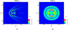 |
Fig. 3. Same as Figure 2, but for Case 2. |
| In the text | |
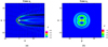 |
Fig. 4. Same as Figure 2, but for Case 3. |
| In the text | |
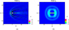 |
Fig. 5. Same as Figure 2, but for Case 4. |
| In the text | |
 |
Fig. 6. Same as Figure 2, but for Case 5. |
| In the text | |
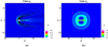 |
Fig. 7. Same as Figure 2, but for Case 6. |
| In the text | |
|
Fig. 8. Thermal (Red), magnetic (black), dynamic (blue) and total (pink) pressures (nPa) at the Sun-Earth line obtained by the global AMR-CESE-MHD model for (a) Case 1, (b) Case 2 and (c) Case 3. The red dashed lines denote the subsolar magnetopause locations (R mg) which are defined by the last closed magnetic field lines and the red dash-dotted lines denote the subsolar bow shock locations (R bs) which are determined by the peaks of the current density in our simulations. |
| In the text | |
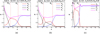 |
Fig. 9. The same as Figure 8, but for (a) Case 4, (b) Case 5 and (c) Case 6, respectively. |
| In the text | |
|
Fig. 10. Positions of the magnetopause and bow shock on the (a) equatorial and (b) meridian planes for Case 1 and Case 4 from our simulations. Red solid and dashed lines denote the positions of the bow shock and magnetopause for Case 1, respectively. Blue solid and dashed lines denote the positions of the bow shock and magnetopause for Case 4, respectively. |
| In the text | |
Current usage metrics show cumulative count of Article Views (full-text article views including HTML views, PDF and ePub downloads, according to the available data) and Abstracts Views on Vision4Press platform.
Data correspond to usage on the plateform after 2015. The current usage metrics is available 48-96 hours after online publication and is updated daily on week days.
Initial download of the metrics may take a while.