| Issue |
J. Space Weather Space Clim.
Volume 8, 2018
|
|
|---|---|---|
| Article Number | A40 | |
| Number of page(s) | 32 | |
| DOI | https://doi.org/10.1051/swsc/2018027 | |
| Published online | 21 September 2018 | |
Research Article
Analysis and interpretation of inner-heliospheric SEP events with the ESA Standard Radiation Environment Monitor (SREM) onboard the INTEGRAL and Rosetta Missions
1
Research Center for Astronomy and Applied Mathematics (RCAAM) of the Academy of Athens, 11527
Athens, Greece
2
Institute for Astronomy, Astrophysics, Space Applications and Remote Sensing (IAASARS), National Observatory of Athens, I. Metaxa & Vas. Pavlou St.
15236
Penteli, Greece
3
Department of Physics, National and Kapodistrian University of Athens, 15784
Athens, Greece
4
Departament de Física Quàntica i Astrofísica, Institut de Ciències del Cosmos (ICCUB), Universitat de Barcelona, Barcelona, Spain
5
European Space Research and Technology Centre (ESTEC), Space Environment and Effects Section, Keperlaan 1, 2200AG
Noordwijk, The Netherlands
* Corresponding author: This email address is being protected from spambots. You need JavaScript enabled to view it.
Received:
16
September
2016
Accepted:
30
July
2018
Abstract
Using two heliospheric vantage points, we study 22 solar energetic particle (SEP) events, 14 of which were detected at both locations. SEP proton events were detected during the declining phase of solar cycle 23 (November 2003–December 2006) by means of two nearly identical Standard Radiation Environment Monitor (SREM) units in energies ranging between 12.6 MeV and 166.3 MeV. In this work we combine SREM data with diverse solar and interplanetary measurements, aiming to backtrace solar eruptions from their impact in geospace (i.e., from L1 Lagrangian point to Earth’s magnetosphere) to their parent eruptions at the Sun’s low atmosphere. Our SREM SEP data support and complement a consistent inner-heliospheric description of solar eruptions (solar flares and coronal mass ejections [CMEs]) and their magnetospheric impact. In addition, they provide useful information on the understanding of the origin, acceleration, and propagation of SEP events at multi-spacecraft settings. All SEP events in our sample originate from major eruptions consisting of major (>M-class) solar flares and fast (>1800 km/s, on average), overwhelmingly (>78%) halo, CMEs. All but one SEP event studied are unambiguously associated with shock-fronted CMEs, suggesting a CME-driven shock acceleration mechanism. Moreover, a significant correlation is found between the SEP event peak and the onset of the storm sudden commencement, that might help improve prediction of magnetospheric disturbances. In general, SEP events correlate better with interplanetary (i.e., in-situ; L1-based) than with solar eruption features. Our findings support (a) the routine use of cost-effective SREM units, or future improvements thereof, for the detection of SEP events and (b) their implementation in multi-spacecraft settings as a means to improve both the physical understanding of SEP events and their forecasting.
Key words: solar flares / coronal mass ejections / solar energetic particles
© M. Georgoulis et al., Published by EDP Sciences 2018
 This is an Open Access article distributed under the terms of the Creative Commons Attribution License (http://creativecommons.org/licenses/by/4.0), which permits unrestricted use, distribution, and reproduction in any medium, provided the original work is properly cited.
1 Introduction
The physical processes resulting in solar energetic particle (SEP) events remain controversial to this day. This is probably because several pieces of the solar eruption puzzle leading to SEPs are still heavily debated or have yet to be put in place. With the first solar flare observed by Lord R. C. Carrington in the mid-19th century and the first solar coronal mass ejection (CME) observations made possible in the early 1970s (e.g., Tousey, 1973; MacQueen et al., 1974), it was not before the 1990s that the decisive role of CMEs was realized in both the understanding and interpretation of heliospheric disturbances and geomagnetic storm activity (Gosling, 1993).
The heliosphere is primarily a plasma environment, fueled by the solar wind in which the interplanetary magnetic field (IMF) is frozen-in and rooted on the rotating Sun, yielding an Archimedean-spiral configuration (Parker, 1958). Therefore, magnetic-energy release by both flares and CMEs leads naturally to acceleration of plasma particles (protons, electrons, and heavier ions) up to relativistic energies, with these SEP events detected in-situ at the spacecraft location, if a suitable magnetic connection exists. However, up to this point, the acceleration properties and the relative roles of magnetic reconnection inside flares and of CME-driven shocks, are still debated. Historically, SEP events have been classified into impulsive and gradual ones (Cane et al., 1986; Reames, 1988, 1999), based on flux and fluence measurements, with the first class attributed to flares and the second to CMEs. Flare-accelerated particles that lead to SEP events can reach geospace only in case of a favorable magnetic field-line geometry, that is, by accessing geospace-connected heliospheric field lines by flare-induced magnetic reconnection in the low solar corona (Claßen et al., 2003). On the other hand, coronal ejecta greatly disturb the heliosphere (Simnett et al., 2002). CMEs faster than the ambient solar wind drive shocks that generate SEP events on timescales much longer than flare timescales, giving them their gradual temporal profile signature (Tylka et al., 2005; Tylka & Lee, 2006). In this case, CME-driven shock-accelerated particles propagate along IMF lines and if the connection between these lines and the observer (e.g. spacecraft) is established, particle flux enhancements are observed at the detectors in space (e.g., Aran et al., 2007). Heliospheric magnetic connectivity plays a crucial role in impulsive (i.e., short-duration, flare-accelerated) SEP events (e.g., Reames, 1999) and an important role in shaping the intensity-type profiles in gradual SEP events associated with CME-driven shocks (e.g., Cane & Lario, 2006), affecting the peak SEP flux and rise times (e.g., Mikić & Lee, 2006).
Inner-heliospheric magnetic connectivity is reflected on the CME’s launch direction for a given heliographic longitude and latitude, as well (Rodríguez-Gasén et al., 2011, 2014). Hence, the CME directionality is another crucial factor for large, gradual SEP events (e.g., Park et al., 2012). Yet, it has been noted by Mikić & Lee (2006) that most CMEs are associated to solar flares and thus it is reasonable to assume that an impulsive component is present in gradual SEP events. Composition measurements of SEP events are essential to distinguishing impulsive from gradual SEP events (Desai and Burgess 2008, and references therein). However, even with such observational evidence at hand, it is often complicated to identify “flare” material in gradual SEP events. This is either because remnant suprathermal particles from previous impulsive events appear as seed particles (Tylka et al., 2005; Klecker, 2013) or because flare accelerated particles get direct access to open magnetic field lines with low-energy particles accelerated by the CME and high-energy particles originating from the flare location (for details, see Klecker, 2013, and references therein). Concerning this second point it is worth mentioning that a similar scenario was also proposed for the highest-energy SEP events that reach an energy of ≥1 GeV and are consequently registered at Earth as ground level enhancements (GLEs). Observations have shown that the so-called prompt component (PC) of GLEs is consistent with flare-accelerated particles, while the delayed one (DC) with CME-shock-accelerated ones (Vashenyuk et al., 2011; Aschwanden, 2012). In addition, recent studies (e.g., Cane et al., 2010; Trottet et al., 2015; Papaioannou et al., 2016) have indicated the extensive presence of the so-called hybrid or mixed SEP events (Kocharov & Torsti 2002) that stem from interconnections between flares and CMEs and may justify the wealth and diversity of the in-situ recorded SEP event profiles.
A viable way to achieve both a physical understanding of solar magnetic eruptions and a predictive capability of them and their heliospheric repercussions is to track them from the Sun to the heliospheric destination of interest. SEP event monitors can be crucial in inversely decoding the likely eruption path, i.e., from the geospace location of observation back to the low solar corona. Major effort has been invested in the development and maintenance of a fleet of spacecraft at the Lagrange 1 libration point (L1) at ~0.99 astronomical units (AU) (e.g., among others: the Advanced Composition Measurements (ACE; Stone et al., 1998), the Solar and Heliospheric Observatory (SOHO; Domingo et al., 1995), and the WIND (see Space Sci. Rev. issue 71 of 1995, February) that provide continuous, near-realtime measurements of the local plasma environment. However, the vast majority of the inner heliosphere cannot be covered by space missions, in spite of targeted past efforts that have set into operations missions such as Helios A1 and B2, Ulysses (Wenzel et al., 1992), and the Solar Terrestrial Relations Observatory (STEREO) (Kaiser et al., 2008). These explorers have greatly advanced our understanding of our local (inner and beyond) heliosphere. At times, identical instruments at different heliospheric vantage points offer simultaneous measurements of single SEP events, providing us with an important tool for understanding the SEP origin, propagation, and acceleration (Agueda et al., 2012; Lario et al., 2013; Dresing et al., 2014; Lario et al., 2016).
In this respect, the European Space Agency’s (ESA) Standard Radiation Environment Monitor (SREM; Bühler et al., 1996; Mohammadzadeh et al., 2003), a heritage instrument with proven, tractable technology, was mounted on several ESA space missions situated in different orbits. The practical size and small weight of SREM units also contributed to this decision by ESA. SREM detects both protons and electrons with energies above 10 MeV and 500 keV, respectively. SEP event measurements acquired from the SREM units allows to, first, analyze SEP events from multiple vantage points and, second, assemble longitudinal distributions of event intensities within the declining phase of solar cycle 23. The calculation of SREM proton and electron differential fluxes is performed via a de-convolution relying on the Singular Value Decomposition (SVD) (Höcker & Kartvelishvili, 1996) method. The resulting inverse technique allows the extraction of the dominant particle flux component from SREM data and the derivation of soft and hard spectra over broad energy ranges (Sandberg et al., 2012).
Tziotziou et al. (2010) first investigated whether SREM SEP event measurements can be used to shed light on the Sun-Earth connection via solar eruptions. They studied 13 SREM SEP events detected by ESA’s INTEGRAL mission (Winkler et al., 2003) between October 2003 and December 2006 and reported that they could be traced back to the Sun, associated with specific solar eruptions. Furthermore, Papaioannou et al. (2011) demonstrated the simultaneous recordings of the SREM SEP event of 20 January 2005 by the INTEGRAL and Rosetta missions (Glassmeier et al., 2007).
This work aims toward a physical interpretation of the observational properties of SREM SEP events. We undertake a study similar to that of Tziotziou et al. (2010), but by using a larger sample of 22 INTEGRAL/SREM SEP events detected between November 2003 and December 2006. For 14 of these events we further combine SREM measurements from ESA’s Rosetta mission, thus studying SEP events observed simultaneously from the two spacecraft. While INTEGRAL is always in geospace, Rosetta was a solar system mission with a continuously varying distance from the ecliptic and the Sun-Earth line. Nonetheless, for the majority of studied events both spacecraft are relatively close to each other with Rosetta being completely separated from INTEGRAL from ~mid 2005 onwards. As a result, SREM measurements shown in this work present identifications of simultaneous recordings of SEP events onboard INTEGRAL and Rosetta, similar to Papaioannou et al. (2011), but further extend to multi-spacecraft SEP events from two well-separated heliospheric vantage points.
Additionally, we attempt a preliminary investigation of the value of using SREM SEP event observations as a means to predict the onset of magnetospheric disturbances. We clarify, however, that the information we use here is not sufficient to address the geoeffectiveness of the corresponding interplanetary CMEs (ICMEs). We leave this issue for future studies utilizing more comprehensive, pertinent information of ICME magnetic field strength, geometry and orientation.
The paper is structured as follows: Section 2 provides a brief description of SREM units, explains a new method of SEP flux inference, and describes the used event dataset. Section 3 describes the solar and interplanetary information complementary to SREM SEP event data that has been utilized to interpret the SEP events. Section 4 proceeds with various aspects of interpretation (including a multi-spacecraft case study) and statistics of events, while Section 5 summarizes the study and findings and offers an outlook on the future utilization of SREM measurements.
2 ESA’s Standard Radiation Environment Monitor
2.1 Instrument description
ESA’s SREM belongs to the second generation of particle detectors in a program established by ESA’s European Research and Technology Centre (ESTEC) to provide minimum intrusive particle radiation detectors on ESA spacecraft for space weather applications.
SREM units such as the one depicted in Figure 1 have been operational onboard STRV-1C, Proba-1, INTEGRAL, Rosetta, GIOVE-B, Herschel and Planck spacecraft. They monitor the radiation environment and provide suitable response functions that can be translated to hazards for the spacecraft and its payload (Evans et al., 2008; Hajdas et al., 2003).
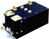 |
Fig. 1. Photograph of the SREM unit onboard the INTEGRAL mission. Each unit weighs 2.6 kg and is contained in a box with linear dimensions 20 × 12 × 10 cm3. |
Each SREM unit is a two-detectors-head configuration that consists of three silicon diodes (D1, D2 and D3) permitting the detection of electron fluxes with energies above 0.5 MeV and of proton fluxes with energies above 10 MeV. The first detector system uses a single silicon diode detector (D3) and the second system includes two silicon diodes (the detectors D1/D2) in a co-axial (telescope) configuration. The pre-amplified detector pulses attributed to incoming energetic particle fluxes are scrutinized by fifteen fast comparators – the SREM channels, eleven for single and four for coincidence events.
SREM channels identify particle energies by the energy deposited in the detector and provide spectral information of the measurements (cf. Table 1) in rather broad and overlapping energy bands (e.g. channels TC1, S12, S13, TC3, S32, S33 and S34). The lower bound in the energy range of the “total count rate” channels of detectors 1 and 3 (TC1 and TC3) corresponds to the threshold penetration of the shields. All channels are sensitive to protons, while the coincidence channels C1–C4, S25 and the S15 can be considered as pure proton channels (Table 1) since only electrons with energies above E > 8 MeV may contribute to their measurements.
List of the SREM channels and the corresponding energy ranges of detected protons and electrons evans (Evans et al., 2008).
SREM units have been calibrated with protons at the Proton Irradiation Facility (PIF) of the Paul Scherrer Institute and with electrons from radioactive sources (90Sr and 60Co) (Hajdas et al., 1996). Moreover, for each SREM unit, a response matrix (RF) has been derived using Geant4 Monte Carlo numerical simulations for omni-directional fluxes of electrons and protons (Agostinelli et al., 2003) supplemented with a GEANT SREM mass model for the corresponding host spacecraft. Figure 2 presents the response functions RF i,q (E) for the INTEGRAL/SREM unit.
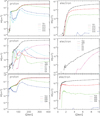 |
Fig. 2. The proton (left column) and the electron (right column) response functions RF i,q (E) of the INTEGRAL/SREM unit for the D1 (top), D1/D2 (middle) and D3 (bottom) group of counters (from Sandberg et al. 2012). |
2.2 Particle flux calculations
The measurements of SREM channels are provided in terms of count rates, C
i
, i = 1 … N
b
(= 15), and are given by the sum (1)
(1)
Each term of the sum is attributed to measurements of the incident proton and electron fluxes. Here, f q (E) denotes the differential omni-directional fluxes in units of [cm−2 MeV−1 s−1] and RF i,q (E) the corresponding response function for q = p, e. The calculation of proton and electron differential fluxes f q (E) requires the solution of Equation (1). This is a Fredholm integral equation of the first kind.
Equation (1) is a classical paradigm of an ill-posed problem, since its solution is not unique and not a continuous function of the counts C i . As a consequence, the numerical solution for the flux presents large variations between adjacent neighboring energy bins and may receive unacceptable negative values.
For the derivation of physically accepted solutions in such problems one may apply known inverse techniques, such as unfolding (Cowan, 1998, p. 152). However, the application of standard approaches for the unfolding of SREM data presents large uncertainties attributed to the large width, the strong overlap of the energy bands that characterize each SREM channel, and the electronproton contamination effects.
For the efficient conversion of SREM counts to charged particle fluxes of high spectral resolution, Sandberg et al. (2012) proposed and implemented a novel technique that applies iteratively the unfolding of measurements using the SVD approach of Höcker & Kartvelishvili (1996) over different proton and electron energy ranges.
As explained already, this inverse method provides both the dominant flux component and soft/hard spectra over different energy ranges. Its use has been validated for unfolded SREM proton fluxes using extensive comparisons with the reference proton dataset of the ESA Solar Energetic Particle Environment Modeling (SEPEM) project (Crosby et al., 2015). This is based on data from the Energetic Particle Sensor (EPS) of NOAA’s Geostationary Operational Environmental Satellites (GOES), cross-calibrated using the IMP-8 Goddard Medium Energy experiment (Sandberg et al., 2014). Comparisons indicated that the developed method is successful and allows the derivation of reliable proton spectra with the highest spectral resolution compared to all known methods that have been applied to SREM data to date. SREM count rate data are accessible online from Paul Scherrer Institute (PSI).3
2.3 Data set description
As stated, a central objective of this study is to determine whether SREM SEP event data can be seamlessly fit into a robust physical framework that includes solar eruptions and subsequent particle acceleration, propagation, and transport through the inner heliosphere and geospace. To this purpose, we have selected a list of 22 SEP events detected by the SREM unit onboard the Earth-orbiting INTEGRAL mission (hereafter labeled I1–I22) and 14 SEP events detected by the SREM unit onboard the interplanetary Rosetta mission (hereafter labeled R1–R14). All events correspond to a roughly three-year period spanning from November 2003 to December 2006. Since Rosetta gained clear separation from Earth in mid 2005, the corresponding majority of SREM SEP events (R1–R10) could be directly correlated with INTEGRAL/SREM SEP events while the remaining four events (R11–R14) offer the opportunity to study multi-spacecraft characteristics of SEP events. As we show in this work, this has proved useful in interpreting each event separately.
Figure 3 shows a sample timeseries of INTEGRAL/SREM (Fig. 3a) and Rosetta/SREM (Fig. 3c) data for the interval 2005 DOY 230–240 (August 18–28), for each of the eight different SREM energy channels with central energy extremes at 12.6 MeV and 166.3 MeV and a nearly even logarithmic distribution. SEP events I18 and R11 are included in this timeseries, by which one may study the relative timing between the two measurements. Aiming to reduce noise and to precisely identify the onset and peak times of the SEP events we have considered 20-minute running averages of these timeseries, for INTEGRAL (Fig. 3b) and Rosetta (Fig. 3d) data, respectively. In what follows, we will use similarly averaged flux timeseries. In the averaged timeseries, onset times of SEP events correspond to times when the proton flux starts increasing monotonically, to exceed a level of three times the value at the reference time. Notice that the 20-minute averaging interval was not chosen arbitrarily: it corresponds roughly to the fastest transit time of energetic particles from Sun to geospace, occurring in case of optimal magnetic connectivity in the inner heliosphere (e.g., Nolte & Roelof, 1973; Krucker et al., 1999; Haggerty & Roelof, 2002). Therefore, using 20-minute averages best captures the evolution of the SEP SREM measurements on large time scales (e.g. several days) and can be used to establish a comparison between the identified SEP events and the evolving magnetospheric disturbances, as those appear in the recordings of interplanetary data.
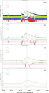 |
Fig. 3. SREM proton flux timeseries registered between August 18 and 28, 2005 for eight different energy channels, from low (12.6 MeV; black) to high (166.3 MeV; red). Unsmoothed INTEGRAL (a) and Rosetta (c) are shown, with their respective 20-minute running averages in (b) and (d). The timeseries include SREM SEP events I18 and R11 (see also Table 2). The INTEGRAL SEP event’s onset time, roughly coinciding with the SEP event recorded onboard Rosetta, is shown by the solid blue line. The INTEGRAL and Rosetta peaks are shown by the dashed blue and brown lines, respectively. |
It should be noted that this method for identifying onset times and peaks of SREM SEP events is not identical to that used by Tziotziou et al. (2010) in more than one way: first, that study used particle counts to identify onsets and peaks, while we use particle flux calculations. Second, no running averages were used in that work. The reason for using particle flux inverted from particle counts, as described in Section 2.2, is to use a validated parameter of physical significance, even at the expense of a somewhat approximate inference of SEP onset and peak times, due to averaging. This has resulted in some differences between the onset and peak times reported for some SEP events that both this study and Tziotziou et al. (2010) include.
The basic properties of our SEP events database are summarized in Table 2. Shown are the SEP event’s onset and peak times, including also a description of the onset time as a function of the SEP energy. In the majority of cases (denoted by S), it seems that the apparent start time of a given SEP event in SREM recordings initiates nearly simultaneously in all energy channels. This may be explained considering that the time-of-flight of 166–18 MeV protons along nominal IMF lines differs by only ~30 min, that is close to the averaging time applied to our data. In several cases, however, the event precedes in lower (L → H) or in higher (H → L) energy channels. This information could potentially provide a hint for the possible source(s) of particle acceleration. Caution in this interpretation is recommended, however, as the non-simultaneous trigger of different energy channels may be due to artifacts (e.g., broad SREM energy ranges, poor statistics). Different parameters, data sets and scenarios need to be accounted for when interpreting this complex acceleration scenario (see the relevant discussion in Section 1), which is a task lying beyond the scope of this work. For consistency with existing literature, SREM SEP events that have also been identified and reported in SOHO, GOES and even STEREO (December 2006) data are also indicated in Table 2. Notice that virtually all SREM SEP events have been previously reported and discussed.
Basic properties of detected INTEGRAL/(I1 – I22) and Rosetta/(R1 – R14) SREM SEP events. Onset and peak times have been inferred manually on a case-by-case basis by the 20-minute averaged proton-flux timeseries – see Figure 3 and related discussion in Section 2.3. Given uncertainties and the complexity of the SEP event temporal profiles, peak times have been rounded to the closest half-hour interval. Furthermore, the peak flux at an E = 12.6 MeV, in protons cm2 MeV−1s−1sr−1, is provided. The * symbol indicates that the peak was marked at the shock. A brief description of the temporal behavior per energy channel is also presented: symbols used are S (simultaneous onset for all energy channels), L → H (onset appearing in lower-energy channels first), and H → L (onset appearing in higher-energy channels first). SEP events detected by both INTEGRAL and Rosetta SREMs are shown in the same line. The angular separation (°) between the two spacecraft is also provided for cases of significant separation. The last column presents published works relying on SOHO, GOES and STEREO data that have reported the SEP events identified also in SREM data. Symbols C, V, P, M1 and M2 refer to specific papers provided underneath the table.
Figure 4 provides a histogram distribution of the rise time of SREM SEP events binned in 6-h intervals and starting from 3 h. The number of INTEGRAL and Rosetta SEP events peaking at times ≤2 h are denoted by the red and blue squares, respectively. From the histogram it appears that SREM SEP events primarily peak within 9–15 h. Secondarily, they range from very impulsive, peaking within ≤3 h, to very gradual, peaking within ~33 h. The results are similar for both INTEGRAL- and Rosetta-detected events. The rise-time distribution extends to exceptionally gradual events peaking at ~57 h. Although the solar origin of SREM SEP events will be discussed in detail in the next section, we note in passing that only a minority of events, namely the most impulsive ones with rise times ≤3 h, are likely to originate from flares in the absence of CMEs (e.g., Cane et al., 2002; Rust et al., 2008). The majority of SEP events can be interpreted by their relation to CMEs, typically via CME-driven shock acceleration (Reames, 1999; Tylka et al., 2005), although one cannot exclude an additional impulsive component in gradual SEP events (Mikić & Lee, 2006).
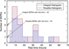 |
Fig. 4. Histogram distribution of the rise times of INTEGRAL/(red) and Rosetta/(blue) SREM SEP events. The numbers of very impulsive SEP events with rise times ≤2 h are shown by the red (INTEGRAL) and blue (Rosetta) square. |
3 Complementary information to SREM SEP event measurements
3.1 Solar data
To pinpoint the solar sources of SREM SEP events we have collected available solar information around the time of interest. Different information has different significance in our analysis: we have categorized it as essential, that is, providing crucial information, and supporting, that is, providing significant but complementary information. The essential solar information comprises the following data sources:
-
Solar soft X-ray flux: To obtain the onset time of the solar flares of interest, NOAA/GOES solar soft X-ray (1–8 Å) flux measurements are used. GOES X-ray flux timeseries do not have spatial information; therefore, solar flares are detected without knowledge of their host active regions. This said, NOAA, via its Space Weather Prediction Center (SWPC), provides a standard active region number and an approximate but reliable heliographic location, at least for the major spikes in the GOES X-ray flux timeseries. Nowadays, besides NOAA/GOES, the Reuven Ramaty High Energy Solar Spectroscopic Imager (RHESSI) mission (Lin et al., 2002), the PROBA-2 (Lawrence et al., 2005) and the Extreme Ultraviolet Variability Experiment (EVE; Woods et al., 2012) onboard the Solar Dynamics Observatory (SDO) allow routine heliographic information of the solar flaring volume (e.g., Hock et al., 2012).
-
CME observations: The Large Angle and Spectrometric Coronagraph (LASCO) CME catalog (Yashiro et al., 2004) is part of the database of the Solar and Heliospheric Observatory (SOHO) mission. CME entries in this and other LASCO-based databases (i.e., the Solar Eruptive Event Detection System (SEEDS; Olmedo et al., 2008) or the Computer Aided CME Tracking (CACTus; Robbrecht & Berghmans, 2004) include detailed information and/or animations of CMEs allowing association with particular solar flares. We particularly focus on (i) the projected CME launch time in the low solar atmosphere, (ii) the linear CME speed, to determine the likelihood of formation of a CME shock (e.g., Mikić & Lee, 2006; Forbes et al., 2006), (iii) the central position angle (CPA) of the CME, to determine whether geospace will likely encounter the resulting ICME, and (iv) the heliographic launch position of the CME, to assess whether the observations support the flaring active region as being also the host of the CME, thus giving rise to a flare/CME eruption (aka eruptive flare).
-
Frequency-time radio spectra: Data from the Radio and Plasma Wave Investigation (WAVES; Bougeret et al., 1995) instrument onboard the WIND mission is used. These data provide information on CME-driven shock formation captured as the so-called Type II bursts, namely observable frequency drifts of emission enhancements in the course of time (see, e.g., Maia & Pick, 2004; Agueda et al., 2009). Time-frequency radio spectra also provide solid evidence for magnetic reconnection in the low solar atmosphere, captured as the so-called Type III bursts, namely nearly instantaneous significant enhancements in multiple frequencies (e.g., Vlahos & Raoult, 1995).
Coupling the above pieces of information completes the essential solar picture for each studied SREM SEP event. An example of essential solar data referring to SEP events I9–I11 (and R3–R5, respectively, from Table 2) is shown in Figure 5.
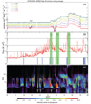 |
Fig. 5. Essential solar information for three INTEGRAL/SREM SEP events (I9–I11) detected in 2005 January. (a) 20-minute running average of the INTEGRAL/SREM flux timeseries between 2005 DOY 10 and 20 (January 10–20). (b) The respective GOES 1–8 Å solar flux, indicating a number of major (>M-class) solar flares. The time interval between the onset and the peak of the three SEP events is indicated by the green-shaded areas. The blue vertical lines correspond to the times of first detection of CMEs with linear speeds >400 km/s, taken by the SOHO/LASCO CME database. (c) WIND/WAVES time-frequency spectrum for the same time period. Notice the detection of several enhanced (Types II and III) radio bursts (the most significant of them indicated by arrows) and, in particular, a strong type II burst (second from right arrow) that coincides with a X2.6 eruptive flare associated with a ultra fast (2596–2861 km/s) halo CME. The I10 SEP event can only be associated with this activity. |
Supporting solar information for SREM SEP events comprises mainly imaging information from the following sources:
-
Full-disk solar magnetograms: Michelson-Doppler Imager (MDI) uninterrupted data (Scherrer et al., 1995) over the entire period of interest is used. In these magnetograms one may crosscheck the source active region location already provided by NOAA information. Moreover, these magnetograms can be used for an overall assessment of the global solar magnetic field. In the simplest possible approach, this is achieved via the Potential-Field Source Surface (PFSS) model of Schrijver & De Rosa (2003). The application is available online via the SolarSoft software package (Freeland & Handy, 1998). One may rightfully argue that the PFSS fields, ignoring electric currents in the solar atmosphere, may at best provide a crude idealization of the true solar magnetic fields. Point taken, the PFSS field can provide a fair assessment of “open” (i.e., closing far out in the heliosphere) solar magnetic field lines. This is because the bases of these lines, known as coronal holes, are topological characteristics that should be detectable even by relatively simple models such as the PFSS (e.g., Rust et al., 2008). Existence of “open” magnetic field lines in the vicinity of a source active region increases the likelihood of an impulsive, flare-driven component in the SEP temporal profiles, pending further scrutiny and validation.
-
Extreme ultraviolet (EUV) and soft X-ray (SXR) images of the Sun: Use of these images may verify the location of the SEP-injecting flare due to the enhanced coronal temperature caused by localized magnetic-energy dissipation. In addition, SXR images offer an empirical tool to detect coronal holes adjacent to the source active region. If existing, these cooler areas appear as patches, veins, or bays in the X-ray images (Rust et al., 2008). Full-Sun SXR images are available from the databases of the X-ray telescope (XRT; Golub et al., 2007) onboard the Hinode satellite and the archived Soft X-ray Imager (SXI; Warmuth et al., 2005) data from GOES. EUV images can be obtained mostly by the databases of the Extreme Ultraviolet Imaging Telescope (EIT; Delaboudinière et al., 1995) onboard the SOHO mission and the Transition Region and Coronal Explorer (TRACE; Handy et al., 1999).
-
Hard X-ray and γ-ray images of the Sun: Intensely flaring active regions appear bright in X- and γ-rays. Emission in such wavelengths is a telltale signal of extensive non-thermal particle populations in the emitting area. Localized, partial-disk solar images in hard X-rays and γ-rays can be obtained from the RHESSI database (Dennis et al., 2007, and references therein).
-
Solar radio images: Eruptive active regions giving rise to CMEs and SEP events should emit in radio, as well, especially in frequencies related to Type II bursts. Eruptive active regions located close to the solar limb have allowed observations of the CME-driven shock actually lifting off as a blob of enhanced radio emission projected on the sky plane (Maia et al., 2000). Such images are acquired by ground-based radioheliographs such as those at Nanc¸ay (Kerdraon & Delouis, 1997) and Nobeyama (Koshiishi et al., 1994).
-
Processed CME images from SOHO/LASCO: From them, one may obtain additional confirmation of a CME’s association with a given source active region and even a frame-by-frame tracking of the CME-driven shock. Two well known automatic CME-tracking utilities, namely, the SEEDS and the CACTus tools, produce results that are available online.
An example of solar supporting information corresponding to SEP event I10 is given in Figure 6. The solar source analysis of Section 4.1 relies, at least, on the essential solar data collected for each SEP event included in Table 2, provided that these data allow a unique temporal association between a SEP event and a generating solar eruption. If no other earthward solar eruption matches the SEP onset time, then we associate the SEP event to the particular eruption. In more complicated settings with multiple eruptive solar flares closely spaced in time, supporting solar data were collected for a number SEP events, to allow for a trusted solar source identification. In any case, we relied our solar source identification either in uniqueness of correlation or in maximum likelihood of correlation, for the more complicated cases. For these cases, in particular, we also cross-check with other published studies that associate SEPs with their solar sources (e.g., Cane et al., 2010; Vainio et al., 2013; Papaioannou et al., 2016). With this approach, we are confident that the solar source association of Table 3 is credible.
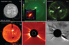 |
Fig. 6. Supporting solar information for INTEGRAL/SREM SEP event I10, detected on 2005 January 15. (a) PFSS-extrapolated SOHO/MDI magnetogram obtained at UT 00:04 on 2005 January 16. Shown in the north-western quadrant is the intense, eruptive NOAA active region (AR) 10720. Magnetic field lines that close back to the Sun are white, while green lines indicate “open” (heliosphere-closing) magnetic connections. (b) Nearly simultaneous SXR image by GOES/SXI showing that NOAA AR 10720 is very bright, indicating flaring activity. The inset shows a nearly simultaneous hard X-ray closeup of the AR reconstructed by RHESSI that also shows flaring emission in the AR. (c) Nearly simultaneous image in the EUV obtained by SOHO/EIT where, again, NOAA AR 10720 is very bright. (d) Full-disk radio image at 17 GHz from the Nobeyama Radioheliograph showing that the AR is also emitting in radio wavelengths. (e) A SOHO/LASCO C2 image providing evidence that the flare triggered in the AR is eruptive, giving rise to a very fast CME. (f) The same image processed by SEEDS and demonstrating the leading edge of the CME (red crosses) and the preceding CME-driven shock (blue crosses). |
Solar sources of detected INTEGRAL/(I1–I22) and Rosetta/(R1–R14) SREM SEP events. In the “Flare” columns we provide the onset date and universal time of the source flares, the flares’ class, the host solar active regions, and the approximate heliographic location of these regions at the flares’ time. In the “CME” columns we provide the linearly projected launch time of the source CMEs, the CMEs’ position angle, their near-Sun linear speed and our assessment on whether these CMEs were preceded by shocks. “Halo” CMEs imply events with a 360° position angle. The confident existence/non-existence of CME-driven shocks is denoted by Y/N, respectively (apparently, N is not used); a question mark casts doubt on the shock existence. Dashes in some columns imply lack of knowledge. Details on CME shock association are provided in Section 4.2.1.
3.2 Interplanetary data
Given the wealth of supporting interplanetary (IP) data that can be used to assess the IP environment of SREM SEP events, we only discuss the essential IP data here, that were extracted and used for the study of each SEP event in Table 2:
-
Measurements from ACE: We use data from multiple instruments onboard the ACE mission at L1. In particular, we collected the Level 2 timeseries of proton density, temperature, and velocity from the Solar Wind Electron Proton Alpha Monitor (SWEPAM; McComas et al., 1998) and the Level 2 timeseries of the Geocentric Solar Ecliptic (GSE) and Geocentric Solar Magnetospheric (GSM) z-components of the solar wind (SW) magnetic field from the mission’s Magnetic Field Experiment (MAG; Smith et al., 1998). The SW proton information was collected in order to determine the crossing of the IP shock at L1. The respective timeseries of the SW B z component were also collected to verify the shock crossing (e.g., Desai et al., 2003), or to determine the crossing, in the case of a data gap in the SW proton information (see, e.g., Fig. 11). We note in passing that, at least in some cases, one may notice after the shock the characteristic SW B z -rotation pattern that is suggestive of a magnetic-cloud crossing from L1 implying a propagating IP magnetic flux rope (Burlaga et al., 1981, and numerous works since).
-
Dst index: Inferences of the Kyoto Geomagnetic Equatorial (Dst) index (e.g., Daglis, 2001) are used to determine the geomagnetic response to a L1 shock crossing and is the safest indicator of whether the terrestrial magnetosphere has evolved into storm conditions as a result of the ICME propagation.
An example of the L1 conditions corresponding to the solar conditions of Figure 5 is given in Figure 7.
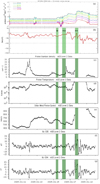 |
Fig. 7. Essential IP information for three INTEGRAL/SREM SEP events (I9–I11) detected in 2005 January. (a) 20-minute running average of the INTEGRAL/SREM flux timeseries between 2005 DOY 10 and 20 (January 10–20). (b) Hourly-averaged timeseries of the Dst index for the same time interval. The information from ACE/SWEPAM includes hourly averages of the SW proton number density (c), temperature (d), and speed (e), while the information from ACE/MAG includes the hourly-averaged GSE (f) and GSM (g) Bz-components. Notice a data gap in the ACE/SWEPAM measurements from midday January 17 to roughly January 19. The green-shaded areas in (b–g) indicate the time interval between the onset and the peak of the three SEP events. |
4 Heliophysical interpretation of SREM SEP events
4.1 Selected cases
In this section we analyze three representative SEP event cases of our sample, one corresponding to a rather well-connected event (I11/R5), showing a rapid rise of particle intensities, one corresponding to a gradual event (I13/R7) and one corresponding to a multi-spacecraft event with a clear separation between the two spacecraft (I20/R13).
4.1.1 2005 January 17 SEP event (I11/R5)
At 06:59 UT on 2005 January 17, NOAA active region (AR) 10720 hosted a major X3.8-class flare (Fig. 8c). The flare was associated with a very fast halo CME with projected launch time at 09:00 UT and a near-Sun linear speed ~2094 km/s. An IP shock manifested as a narrow-drift Type II burst associated with this CME was detected at 09:11 UT (Fig. 8d; see also Hillaris et al., 2011). At the time of the eruption, the approximate heliographic location of the AR was N13 W30 (north-western quadrant; Fig. 9a). This means that nominally the AR was in favorable magnetic connectivity with Earth. Meanwhile, the global solar magnetic field adjacent to the AR did not show evidence of “open” magnetic field lines (Fig. 9b).
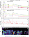 |
Fig. 8. Solar coronal conditions between 2005 January 17 and 25, including SEP event I11/R5. (a) 20-minute running averages of the INTEGRAL/SREM particle flux timeseries, (b) 20-minute running averages of the Rosetta/SREM particle flux timeseries, (c) GOES 1–8 Å solar X-ray flux and (d) WIND/WAVES frequency-time radio spectrum. The vertical solid black line indicates the onset time of the flare related to the SEP events source eruption. The flare information is annotated in (c) and the source CME information is annotated in (d). The arrow in (d) indicates the approximate start time of a CME-associated Type II radio burst. The red vertical dashed line at 10:15 UT on January 17 indicates the SEP event onset time observed first by the highest energy channel of INTEGRAL/SREM while the lowest energy channel detected the onset at 12:51 UT (second black vertical dashed line). It was also the lowest energy channel of Rosetta/SREM which was the last channel to detect the SEP event (11:48 UT, first black vertical dashed line). The colors used in (a) and (b) correspond to the different energy channels of the SREM detectors. |
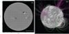 |
Fig. 9. Solar disk and the global solar magnetic field on 2005 January 17. (a) Full-disk solar magnetogram from SOHO/MDI, as obtained by Solar Monitor (Gallagher et al., 2007). The source NOAA AR 10720 is visible in the north-western quadrant. (b) The global PFSS-extrapolated solar magnetic field early on 2005 January 17. Closed field lines are white while positive- and negative-polarity “open” field lines are colored magenta and green, respectively. |
At 10:15 UT on 2005 January 17, INTEGRAL/SREM detected a SEP event onset (Fig. 8a). The enhancement was detected in SREM energy channels, with the highest-energy channel (166.3 MeV) registering it first. The lowest-energy channel (12.6 MeV) detected the SEP event onset at 12:51 UT. Virtually simultaneously, Rosetta/SREM also detected an SEP event onset, also via its highest-energy channel (Fig. 8b). The last channel to detect the SEP event was the lowest-energy Rosetta/SREM channel, at 11:48 UT. The temporal profiles of both SREM SEP events were quite similar, albeit smoother in the Rosetta/SREM recordings.
Recounting the events of 2005 January 17 in a more general context, a particularly complex picture emerges: an even faster halo CME than the one above occurred at 09:54 UT (linear speed of ~2547 km/s) (Papaioannou et al., 2010; Hillaris et al., 2011). Despite ACE/SWEPAM exhibiting data gaps and low-resolution data and magnetic field measurements at 1 AU at the time, Papaioannou et al. (2010) were able to track the propagating ICME structures to the extent possible. Earlier on January 17, at 07:52 UT, a forward shock was detected as a result of CMEs released from the Sun two days earlier. The passage of this shock was followed by an unusually extended region exhibiting sheath-like characteristics, observed for ~1.5 days thereafter with highly variable magnetic-field magnitude and direction, typical of high proton temperatures (see Fig. 3 of Papaioannou et al., 2010). In addition, Hillaris et al. (2011) provided a thorough analysis of the CME-CME interaction, caused by the overtaking of the preceding, slower, CME of 09:00 UT by the faster event of 09:54 UT. Near-relativistic (NR) electrons were observed by ACE/EPAM but their analysis shows that they could not have been accelerated by the interacting CMEs. Instead, acceleration should have taken place impulsively in regions where particles had ready access to solar wind magnetic field lines.
As to the I11/R5 SREM SEP event, the overall picture above implies the following: first, the earlier registration of the higher-energy channels at geospace, points to the favorable magnetic connectivity with the source AR. As soon as the CME magnetic field lines reconnect with the heliospheric ones, shock-accelerated particles “leak” with the fastest apparently reaching Earth first (Mikić & Lee, 2006). Given the favorable heliographic location of the source region and the magnitude of the associated flare, one cannot rule out an impulsive, flare-related contribution to the corresponding SEP event. Indeed, the back-mapping of the timing analysis furnished in Hillaris et al. (2011) correlates the release of NR electrons to open magnetic field lines signified by Type III bursts – this indicates that the assessment of the PFSS model of Figure 9b may be inaccurate. Second, the similarity between the SEP temporal profiles suggests that Rosetta should, at the time of detection, be close to geospace. Figure 10 shows the unsmoothed recordings of INTEGRAL/SREM (panel on the left), the position of INTEGRAL and Rosetta (middle panel) and the Rosetta/SREM measurements. Rosetta was indeed quite close to Earth (its first Earth flyby completed on 2005 March 4) and slightly further from the Sun in terms of heliocentric distance. This also explains the slightly smoother profile of the Rosetta/SREM SEP event.
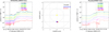 |
Fig. 10. Calibrated, unsmoothed INTEGRAL/(left panel) and Rosetta/(right panel) SREM timeseries for SEP event I11/R5. The solid line in both panels denotes the onset of the SEP event at the respective spacecraft. The middle panel shows the positions of Rosetta (red) and INTEGRAL (blue) spacecraft relative to the Sun (yellow), with distances shown in AU. |
Both INTEGRAL/ and Rosetta/ SREM SEP events peaked simultaneously and for all energy channels at ~19 UT on 2005 January 17, ~9 h after the onset of the event (Figs. 11a and b). As can be seen in Figures 11c and d, this simultaneous peak in the SEP intensity coincides with a notable increase in the local IMF amplitude at L1. Indeed, this SEP event was preceded by the passage of an IP shock and its corresponding ICME, affecting the rising phase of the proton event (Lario et al., 2009). The declining phase lasted considerably longer, until the early hours of 2005 January 19.
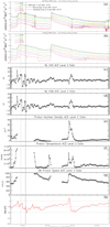 |
Fig. 11. IP conditions between 2005 January 17 and 25, including SEP event I11/R5. (a) 20-minute running averages of the INTEGRAL/SREM particle flux timeseries, (b) 20-minute running averages of the Rosetta/SREM particle flux timeseries, ACE/MAG Bz-components in GSE (c) and GSM (d) coordinates and ACE/SWEPAM measurements of proton number density (e), proton temperature (f) and SW proton velocity (g). The respective definitive Dst-index values are given in (h). The three vertical lines indicate the times of the SEP event’s peak (dashed), the shock crossing from L1 (solid), and the onset of the magnetospheric disturbance (dotted). All respective dates and times are annotated in (a). |
The shock-front of the propagating ICME crossed L1 ~9 h after the peak in particle flux, at ~05 UT on 2005 January 18, as was deduced only by the GSE and GSM B z -components (Figs. 11c and d), given the ACE/SWEPAM data gaps (Figs. 11e–g). This is the most likely shock passage time given the steepness of the local gradient in the timeseries of B z . The timing of the shock-front L1 crossing is consistent with the findings of Papaioannou et al. (2010) (see their Fig. 5 and relevant discussion), who used short-term neutron monitor decreases – known as Forbush decreases (Belov, 2008) – to identify the crossing time. A storm sudden commencement ensued ~2 h after the shock crossing, at ~07 UT on 2005 January 18. As explained above, the magnetosphere was already disturbed at the time (Dst ~ −50 nT) but the Dst index dipped further to storm-time conditions. The disturbance peak was at Dst ~ −110 nT and was reached at ~09 UT on 2005 January 18. The magnetosphere remained in storm-time conditions for ~2 more days, gradually emerging from it in the early hours of 2005 January 20. Notice that late on 2005 January 21 the magnetosphere reached storm-time conditions again due to the arrival of the IP disturbances of another intense ICME originating from an eruptive X7.1 flare, clearly seen in Figure 8. The resulting SEP event (Fig. 11) was one of the strongest in solar cycle 23, giving rise to Ground Level Enhancement (GLE) 69 (e.g., Bieber et al., 2005). This event originated also from NOAA AR 10720 and corresponds to SEP event I12/R6, included in the present work.
A notable SEP event feature often discerned at the time of shock passage from western source-region locations is a secondary peak in the particle flux. In our case the peak is visible in both INTEGRAL/ and Rosetta/SREM data (Figs. 11a, and b). For eastern source locations, and hence mostly gradual events, the shock crossing matches the primary peak in particle flux much better. In this case particles that leak upstream mostly miss geospace so that the shock ensemble with part of the SEP population trapped in it, apparently via waves (e.g., Ng & Reames, 1994; Reames, 1999), arrive together. For western sources, upstream-leaked particles reach Earth prior to the shock forming the primary peak so the shock arrival and its trapped SEP population give rise to the secondary peak thereafter. The shock’s influence on gradual SEP intensity-time profiles has been interpreted in long-standing works (see, e.g., Lario et al., 1998, and references therein).
4.1.2 2005 May 13 SEP event (I13/R7)
Eruptive solar active region NOAA AR 10759 hosted a M8-class flare at 16:13 UT on 2005 May 13 (Fig. 12c. A well-formed shock was observed in conjunction (Fig. 12d) and a fast halo CME was detected with a projected launch time at 16:40 UT and a near-Sun speed of ~1689 km/s (see also Bisi et al., 2010). At the time of the eruption, the heliographic location of the AR was N12 E10 (north-eastern quadrant; Fig. 13a). There is some evidence of “open” magnetic field lines relatively close to the AR (Fig. 13b. The M8 solar flare was fairly gradual, with an extended rise time of 44 min and an associated Type III burst (start time: 16:40; end time: 17:00). Furthermore, a Type II radio burst, associated to the fast propagating CME, started on 13 May 2005 at around the onset of the CME (~16:38 UT, according to Bisi et al., 2010). As a result, a relatively strong SEP event was recorded at L1 (with peak energy ~80 MeV, according to Cane et al., 2010).
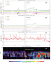 |
Fig. 12. Solar coronal conditions between 2005 May 10 and 18, including SEP event I13/R7. (a) 20-minute running averages of the INTEGRAL/SREM particle flux timeseries, (b) 20-minute running averages of the Rosetta/SREM particle flux timeseries, (c) GOES 1–8 Å solar X-ray flux and (d) WIND/WAVES frequency-time radio spectrum. The vertical solid black line indicates the onset time of the flare related to the SEP events source eruption. The flare information is annotated in (c) and the source CME information is annotated in (d). The first dashed black line at 18:56 UT on May 13 indicates the SEP event onset time observed first by the lowest energy channel of INTEGRAL/SREM. It was also the lowest energy channel of Rosetta/SREM which was the first channel to detect the SEP event (20:51 UT, second black vertical dashed line). The colors used in (a) and (b) correspond to the different energy channels of the SREM detectors. |
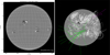 |
Fig. 13. Solar disk and the global solar magnetic field on 2005 May 13. (a) Full-disk solar magnetogram from SOHO/MDI, as obtained by Solar Monitor. The source NOAA AR 10759 is visible in the north-eastern quadrant. (b) The global PFSS-extrapolated solar magnetic field at about the same time. Closed field lines are white while positive- and negative-polarity “open” field lines are colored magenta and green, respectively. |
At 18:56 UT on 2005 May 13, INTEGRAL/SREM detected an SEP event onset, first by its lowest-energy channel (Fig. 12a). Higher-energy channels followed; for example, the 38 MeV channel registered it at 20:20 UT. The SEP event barely appeared in the INTEGRAL/SREM highest-energy channel (166.3 MeV). The Rosetta/SREM detected the onset of the event at 20:51 UT on 2005 May 13, also with its lowest-energy channels first (Fig. 12b). The two profiles from INTEGRAL/ and Rosetta/SREMs are qualitatively similar, with smoother profiles for the Rosetta/SREM, as in the previous case (Sect. 4.1.1). There are two differences, however: (i) two Rosetta/SREM channels (38 MeV and 55 MeV) registered the onset later (00:40 UT on 2005 May 13), while the rest of the energy channels seemed to register the onset nearly simultaneously, and (ii) the SEP event was clearly registered in all energy channels of the Rosetta/SREM, even in the highest ones. Figure 14 shows the actual recordings of both INTEGRAL and Rosetta/SREM, as well as the spacecraft position.
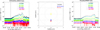 |
Fig. 14. Calibrated, unsmoothed INTEGRAL/(left panel) and Rosetta/(right panel) SREM timeseries for SEP event I13/R7. The solid line in both panels denotes the onset of the SEP event at the respective spacecraft. The middle panel shows the positions of Rosetta (red) and INTEGRAL (blue) spacecraft relative to the Sun (yellow), with distances shown in AU. |
The north-eastern heliographic location of the source AR tends to explain both the precedence of the lowest-energy channels and the SEP event’s temporal profile. Indeed, given the source location, faster, higher-energy protons may have missed geospace.
Following a complicated, quite gradual rise-phase profile, the particle flux peaked at ~02:30 UT on 2005 May 15 for INTEGRAL/SREM (Fig. 15a), ~33 h after its onset. The peak was virtually simultaneous in all energy channels. Given that the inner heliosphere seemed rather quiescent at the time of the event, this temporal complexity should be attributed to complexity in the parent eruption: eruption asymmetries (e.g., Liu et al., 2009) of SEPs stemming from the ICME flank (Heras et al., 1995; Aran et al., 2007; Rouillard et al., 2011) are likely contributors. For the Rosetta/SREM, the SEP event peaked at ~12 UT on 2005 May 15, ~39 h after its onset (Fig. 15b. This rise-time discrepancy is hard to reconcile; however, one might argue that the propagating ICME should be very inhomogeneous at relatively short length scales for such discrepancies to be realized between two not too distant observation locations. The complexity of this particular ICME has been already discussed (e.g., Bisi et al., 2010, and references therein), while Dasso et al. (2009) proposed the presence of two, interacting, magnetic clouds (MCs) within the complex ICME envelope. We consider it quite likely that this ICME complexity gives rise to the inhomogeneity present in the SREM SEP time profiles.
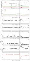 |
Fig. 15. IP conditions between 2005 May 10 and 18, including SEP event I13/R7. (a) 20-minute running averages of the INTEGRAL/SREM particle flux timeseries, (b) 20-minute running averages of the Rosetta/SREM particle flux timeseries, ACE/MAG Bz-components in GSE (c) and GSM (d) coordinates and ACE/SWEPAM measurements of proton number density (e), proton temperature (f) and SW proton velocity (g). The respective definitive Dst-index values are given in (h). The three vertical lines indicate the times of the SEP event’s peak (dashed), the shock crossing from L1 (solid), and the onset of the magnetospheric disturbance (dotted). All respective dates and times are annotated in (a). |
As expected for eastern source locations, the shock passage from L1 occurred nearly simultaneously with the particle flux peak, at ~02 UT on 2005 May 15 (Figs. 15c–g). Given the complex parent particle source, the shock was strong in both ACE/MAG and ACE/SWEPAM measurements. At virtually the same time (~01:30 UT on 2005 May 15; Fig. 15 h) a storm sudden commencement occurred with the Dst index reaching extreme levels (~ −250 nT) within hours. Storm recovery was slow thereafter, achieving Dst > −50 nT not before the late AM hours of 2005 May 18.
4.1.3 2005 September 13 SEP event (I20/R13)
In September 2005, a single active region, NOAA AR 10808, produced a total of 9 X–class, 15 M–class, and many minor flares during the period September 7–13, as it was rotating from the eastern limb to the central meridian. This exceptionally active period premiered with an X17.0 flare at 17:17 UT on 2005 September 7, one of the largest X-ray flares ever recorded. During this period there were also five major frontside CMEs along with several other smaller CMEs, all originating from the same source (Wang et al., 2006; Papaioannou et al., 2009).
At 19:19 UT on 2005 September 13, a X1.5 solar flare originated in NOAA AR 10808, at heliographic location S11 E05 (Figs. 16 and 17 – see also Tziotziou et al., 2010). This flare was associated with a fast (~1866 km/s) halo CME that was marked at 19:36 UT. Type III bursts were identified from 19:50–20:00 UT on the same day, with a flare-related SEP energy at geospace peaking at 7 MeV (Cane et al., 2010). A Type II burst was also identified by Wang et al. (2006) at 20:20 UT, that was debated by Cane et al. (2010) who could not find clear evidence for it in the dynamic spectra.
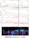 |
Fig. 16. Solar coronal conditions between 2005 September 7 and 18, including SEP event I20/R13. (a) 20-minute running averages of the INTEGRAL/SREM particle flux timeseries, (b) 20-minute running averages of the Rosetta/SREM particle flux timeseries, (c) GOES 1–8 Å solar X-ray flux and (d) WIND/WAVES frequency-time radio spectrum. The vertical solid black line indicates the onset time of the flare related to the SEP events source eruption. The flare information is annotated in (c) and the source CME information is annotated in (d). The dashed black line at 23:02 on September 13 indicates the SEP event onset time observed first by the lowest energy channel but simultaneously for both INTEGRAL/SREM and Rosetta/SREM. The colors used in (a) and (b) correspond to the different energy channels of the SREM detectors. |
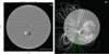 |
Fig. 17. Solar disk and the global solar magnetic field on 2005 September 13. (a) Full-disk solar magnetogram from SOHO/MDI, as obtained by Solar Monitor. The source NOAA AR 10808 is visible in the southern hemisphere, close to the central meridian. (b) The global PFSS-extrapolated solar magnetic field at about the same time. Closed field lines are white while positive- and negativepolarity “open” field lines are colored magenta and green, respectively. |
The corresponding SEP event was detected by both INTEGRAL and Rosetta SREMs nearly simultaneously, at 23:02 UT on 2015 September 13. Just like the previously studied event in the eastern hemisphere (Sect. 4.1.2), different energy channels in INTEGRAL/SREM registered different onset times (Fig. 16). Moreover, the SEP event was barely, if at all, detected at the highest-energy channels of INTEGRAL/SREM. In cases such as this, the near-Earth spacecraft most likely establishes connection with a generally weak flank (in terms of acceleration efficiency) of the CME-driven shock and only later does it connect with parts of the shock that are able to accelerate particles more effectively (Aran et al., 2007). This time, however, the Rosetta/SREM SEP profile was different, with a nearly simultaneous event detection and presence in all energy channels.
From the global PFSS magnetic field at the time of the event (Fig. 17b one notices the clear presence of open magnetic field lines adjacent to the source NOAA AR 10808. If any or some of these lines were connected to geospace, an impulsive, flare-related SEP component should be detected within a few tens of minutes from the flare triggering. This did not occur, apparently due to the sub-optimal heliographic location of the source active region.
At that time, Rosetta was at a radial distance of ~1.34 AU from the Sun, at ~50° east from the Sun-Earth line, while INTEGRAL was typically much closer to Earth’s position (Fig. 18). This relative position can account for a situation in which Rosetta encounters the CME-driven shock nose while INTEGRAL encounters its western flank. This is supported also by the analysis of Wang et al. (2006) – see Figure 6 of that paper, in particular. This further provides reasonable grounds for a more prolonged Rosetta/SREM SEP profile, particularly at higher energies, which can be deduced from Figures 16 and 18.
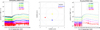 |
Fig. 18. Calibrated, unsmoothed INTEGRAL/(left panel) and Rosetta/(right panel) SREM timeseries for SEP event I20/R13. The solid line in both panels denotes the onset of the SEP event at the respective spacecraft. The middle panel shows the positions of Rosetta (red) and INTEGRAL (blue) spacecraft relative to the Sun (yellow), with distances shown in AU. |
As also expected by the relative positions of the two spacecraft with respect to the SEP event’s solar source, Rosetta is better connected to the shock at the beginning of the event, which leads to a faster increase of the particle intensities compared to the INTEGRAL/SREM SEP observation. This is evident in Figure 19 with the Rosetta event peaking at ~06 UT on 2015 September 14 and the INTEGRAL event peaking at ~15 UT on the same day. About 18 h later, at ~09 UT on 2005 September 15, the corresponding shock crosses L1 causing an increase in the solar wind velocity from ~600 km/s to ~900 km/s and a ~25-fold increase in the solar wind proton temperature. Shortly after the shock, at ~10:30 UT, the corresponding magnetospheric disturbance kicks in, decreasing the Dst-value from a moderately disturbed −38 nT to a storm-time minimum of ~ −90 nT. Hence, this was not an extreme storm case, with the magnetosphere recovering at about midday on 2005 September 16. In terms of the K p index, there was a peak of 7 that marked unsettled conditions, that however faded to 4, early on 2005 September 16 (Papaioannou et al., 2009).
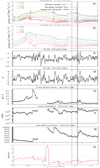 |
Fig. 19. IP conditions between 2005 September 7 and 18, including SEP event I20/R13. 20-minute running averages of the INTEGRAL/SREM particle flux timeseries, (b) 20-minute running averages of the Rosetta/SREM particle flux timeseries, ACE/MAG Bz-components in GSE (c) and GSM (d) coordinates and ACE/SWEPAM measurements of proton number density (e), proton temperature (f) and SW proton velocity (g). The respective definitive Dst-index values are given in (h). The three vertical lines indicate the times of the SEP event’s peak (dashed), the shock crossing from L1 (solid), and the onset of the magnetospheric disturbance (dotted). All respective dates and times are annotated in (a). |
4.2 Solar sources and interplanetary consequences
4.2.1 Synoptic results
Using the essential and supporting information of Section 3 and the reasoning of Section 4.1 we have first attempted to pinpoint the solar sources of all detected SREM SEP events and their properties. The results are summarized in Table 3.
Similar tables for SREM data have been previously published by Tziotziou et al. (2010), and are also inferred by Papaioannou et al. (2016), Cane et al. (2010) and Vainio et al. (2013), among many other studies using multiple data sources. We notice an overall agreement between solar sources for common events, despite the different SEP event databases. It becomes evident, therefore, that SREM SEP events can also be used for providing an overall, consistent picture of the ICME propagation through the inner heliosphere. Furthermore, SREM units provide the unique opportunity to identify and analyze multi-spacecraft events during the declining phase of solar cycle 23. At that time, Ulysses was the only other available spacecraft capable of such studies: however, at a heliocentric distance close to its aphelion (~5.4 AU) and an unfavorable angular separation from Earth, such analyses would be challenging and complicated. In fact, only a few such analyses have been performed using such data by Ulysses (Lario et al., 2008; Malandraki et al., 2009).
Another straightforward conclusion from Table 3 is that virtually all SREM SEP events (at least 21 out of 22, or ~95%) seem to be associated with well-defined, shock-fronted CMEs. To determine whether a source CME formed a shock front we relied on, first, the CME speed and, second, observations of Type II bursts from Wind/WAVES data. For CME speeds well above the speed of the fast solar wind (~800 km/s), a shock should be expected. In addition, for all but one of our source CMEs, Wind/WAVES has identified Type II bursts whose properties are presented at NASA’s CDAW Data Center.4
For SEP event I17/R10, our only exception, there was no near-Sun evidence for a CME-driven shock. However, the source eruption took place at the farside of the Sun, therefore neither a flare nor a host active region were registered. This particular event is not included in the studies cited above, although Cid et al. (2012) assigned it to a M3.7 flare that occurred in NOAA AR 10792 on July 27, 2005, at 05:02 UT. The active region at the time was located at N11E90. Moreover, the corresponding CME was a backside halo with speed 1187 km/s, according to these authors. However, in our data, event I17/R10 started as an extremely gradual event early on July 26, 2005, on both INTEGRAL/ and Rosetta/SREM units (Table 2). Hence, we cannot assign it to a solar eruption that occurred on the next day. It is safe to say, nonetheless, that the event was connected to a farside solar eruption, hence it is quite likely that the CME-driven shock was missed in coronal time-frequency radio spectra. The CME’s high linear speed (>1200 km/s) in our interpretation, however, leaves little doubt that there should be an associated CME-driven shock.
Figure 20 shows the approximate source active region heliographic locations at the time of the source eruptions for 20 out of the 22 SEP event cases of Table 3 (that is, excluding SEP events I16 and I17/R10). In 15 out of 20 SEP events (75%) the host active regions were located in the western solar hemisphere, with more than half (11/20) of the host regions located in the north-western quadrant. This is consistent with the well-accepted fact of the favorable magnetic connectivity with geospace from the western solar hemisphere (see, e.g., Fig. 2 of Gopalswamy et al., 2011), and particularly the north-western quadrant. Conversely, 5/20 (25%) of the host active regions were located in the eastern solar hemisphere at the time of the source eruptions. Some of them (2/5) were located close to the solar-disk center, at central meridian distances (CMD) ≤10°. One case (event I4) was at relatively high eastern CMD, while for two cases (I19/R12 and I21/R14) the assessed host active regions were located on, or close to, the eastern solar limb at the time of the source eruptions. While we have a clear CME-driven shock evidence for both events, LASCO was not operating at the time. For I19/R12, however, a superfast CME with speed ~2400 km/s has been reported by the ground-based Mk4 K-Coronagraph of the Mauna Loa Solar Observatory (Malandraki et al., 2008). For I21/R14, one asserts that another fast CME should have also been launched, given the sheer size of the source flare (X9.0 – see Table 3). The reason why these SEP events were observed from geospace several hours after the eruptions’ onset, in spite of their eastern-limb source location, should therefore be the extreme inner-heliospheric disturbance that these eruptions caused, supplying the entire upstream region with major proton leakages.
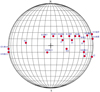 |
Fig. 20. Approximate heliographic locations of the host active regions at the time of the source eruptions for the SREM SEP event solar sources of Table 3. The various SEP event labels of Tables 2 and 3 are also indicated. The solar disk center is indicated by the cross. |
Table 4 summarizes the assessed impact, at L1 and the geospace, of the eruptions that gave rise to the SREM SEP events of Tables 2 and 3. Notice that a geospace disturbance (not necessarily geoeffectiveness,5 though) exists for the vast majority of events, with Dst indices ranging between a few tens to nearly 250 nT southward. Somewhat different behavior is exhibited by SEP events I14/R8, I19/R12, and I21/R14. These cases are briefly discussed below:
-
SEP event I14/R8 was not associated with a CME. Neither a shock passage at L1, nor a discernible magnetospheric disturbance could be detected. For this event, it is likely that a slow and narrow CME occurred but went undetected as the source region was at the western solar limb and perhaps slightly beyond that in the farside. Therefore, this SEP event seems to be a pure consequence of the favorable magnetic connectivity of the host region with geospace.
-
SEP event I19/R12 could not be unambiguously associated with a shock passage at L1, although a magnetospheric disturbance clearly kicked in and the Dst index abruptly dipped to −139 nT at the peak. There is a possibility that the shock went undetected because ACE/SWEPAM measurements had a data gap at the time of the possible crossing; ACE/MAG measurements, on the other hand, could not be interpreted unambiguously. Notice that the host active region was at the eastern solar limb at the time of the source eruption.
-
SEP event I21/R14, with a source region also at the eastern limb, was associated neither with a CME nor with a shock passage at L1. ACE/SWEPAM measurements also experienced gaps during the time of the possible crossing and ACE/MAG measurements were not conclusive. This is probably because the IMF was already quite disturbed at the time, so the shock, if any, probably went undetected. Contrary to SEP event I19/R12, the magnetosphere was already disturbed (Dst ~ −55 nT at peak) in this case, so the source CME was not particularly geoeffective.
Interplanetary environment of detected INTEGRAL/(I1–I22) and Rosetta/(R1–R14) SREM SEP events. Included are the times of the assessed shock passage from L1, those of the ensuing magnetospheric disturbance, and those of the peak Dst index during the disturbance, including the value of the index. We also provide time intervals and index-value ranges when the Dst index fluctuates around the peak. Dashes in some columns imply lack of knowledge.
The above exceptions given, the parent activity that gave rise to the SREM SEP events in our sample could be, to a larger or lesser degree, backtraced from 1 AU to the Sun. More importantly, we were able to largely agree in our interpretation of SREM SEP events with the interpretations provided by analyzing the data of other, primarily science-oriented, instruments (Sect. 4.1). This further attests to the reliability of SREM measurements.
4.2.2 Statistical correlations and predictive ability
Having established a defensible physical picture for SREM SEP events, we now investigate whether this information can be used to advance our understanding of the propagating eruption products throughout the inner heliosphere. We notice that, first, SEP events cannot be used for the prediction of solar eruptions (i.e., flares and/or CMEs), since they are injected after their onset. Second, SEP events cannot be used for an assessment of the geoeffectiveness of ICMEs, given that the decisive factors for this are ICME speed, magnetic configuration, geometry and orientation. We, therefore, investigate whether SEP event detection can help predict when to expect the IP shock and/or the ensuing geomagnetic disturbance, regardless of geoeffectiveness.
The arrival of ICMEs at geospace is currently being pursued either by applying various aerodynamic drag-force models near-Sun CME measurements (e.g., Vršnak et al., 2010; Subramanian et al., 2012, and references therein) or, more recently, by triangulation of information provided by STEREO data (e.g. Davis et al., 2012; Möstl & Davies, 2013). As Figure 21 shows, the location of the host active regions, quantified by means of the regions’ CMD at the time of eruptions, is insufficient to predict the onset of the respective storm sudden commencement, assuming that the shock passage at L1 is observed and reported. Indeed, the average time lapse between shock passage and the onset of the magnetospheric disturbance is (2.65 ± 2.30) h, showing poor correlation coefficients with the host regions’ CMD. In this exercise, SEP events are not included in the picture. Including them and correlating INTEGRAL/SREM SEP event properties with basic eruption properties (only INTEGRAL data are used here as the INTEGRAL spacecraft is always in geospace) as a function of the host regions’ CMD leads to Figure 22.
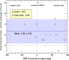 |
Fig. 21. Time difference between the shock passage at L1 and the onset of the storm sudden commencement as a function of the host regions’ CMD at the time of the source eruption. Information stems from Tables 3 and 4. The solid blue line indicates the mean of the time difference and the purple-shaded area indicates the standard deviation around this mean. Dotted lines in each plot indicate the solar limbs (east/west for CMD = −90°/90°) and the central meridian (CMD = 0°). The linear (Pearson) and rank order (Spearman) correlation coefficients are also provided. |
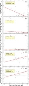 |
Fig. 22. Timing between INTEGRAL/SREM SEP events and various source eruption properties near the Sun and at geospace. All correlations are shown as a function of the CMD of the source solar active regions. Shown in the ordinates are (a) the SEP event rise time, (b) the time interval between the flare onset and the SEP event onset, (c) the interval between the projected source CME launch time and the SEP event onset, (d) the interval between the SEP event peak and the shock crossing time at L1, and (e) the interval between the SEP event peak and the onset of the storm sudden commencement. Solid red lines in all plots correspond to the linear least-squares best fits of the shown data points. The details and goodness of these fits (χ 2-statistic) are shown in Table 5. Dotted lines in each plot indicate the solar limbs (east/west for CMD = −90°/90°) and the central meridian (CMD = 0°). The linear and rank order correlation coefficients are also provided for each plot. The outlier in (b) and (c) corresponds to the source-eruption information of event I4 – see text for details. |
Let us clarify that the statistics of Figures 21 and 22 do not include SEP events I3, I8, I10, I13, I15 and I16. This is because, as also noticed in Table 2, these events seem to have their maxima associated with local shocks. To cross-check this assessment we have consulted the University of Helsinki Database of IP shocks, available at http://ipshocks.fi/. Three of our SEP events (I3, I10 and I13) indeed have their maxima associated to local shocks. For the remaining three events (I8, I15, I16) no shock was conclusively found in the University of Helsinki database, but their temporal profiles showed peculiar features (e.g., local spikes, low-energy diffusion, etc.), so they were removed from this statistical investigation.
Figure 22 correlates the host active regions’ CMD with the SEP event’s rise times (Fig. 22a) and this CMD with the time intervals between: the SEP event onset and the source flare onset (Fig. 22b, the SEP event onset and the linearly projected launch time of the source CME (Fig. 22c, the shock crossing at L1 and the SEP event peak (Fig. 22d , and the time of the storm sudden commencement onset and the SEP event peak (Fig. 22e). The SREM SEP events statistics of Tables 2–4 are sufficient for some rudimentary quantitative processing of these correlations.
In brief, Figure 22 confirms that geospace-affecting SEP events are statistically more likely to occur as the host active region is located more westward at the time of the injection (Fig. 22a). In these cases, SEP events also reach geospace faster (Figs. 22b and c). In addition, westward-injected SEP events peak increasingly in advance of the shock crossing at L1 and the kick-in of the geomagnetic disturbance, with their peak time correlating better (but still in a statistical sense, that is, with sizable uncertainties present) with shock-crossing time and geomagnetic disturbance onset (Figs. 22d and e, respectively). In spite of the fact that the causal sequence of events clearly becomes more intuitive when SEP events are included in the eruption-propagation cadre (cf. Figs. 21 and 22), not all correlations involving SEP events are statistically significant. One might claim potentially significant correlations only for the bottom two plots of Figure 22, as the notably lower χ 2-values for these plots also show (Table 5). Of them, the correlation between the host region location and the time difference between the SEP events’ peak and storm sudden commencement (Fig. 22e) seems more reliable. Figures 22d and e present evidence that SEP events correlate better with the IP features of the source eruptions than with their solar ones (correlation coefficients 0.50–0.63 and 0.72–0.76 for Figs. 22d and e, respectively), apparently because ICME propagation and particle transport in the inner heliosphere undergo in-situ modulations that act to blur the “memory” of the details of these eruptions’ onset and initial propagation in the lower solar corona. The only solar information that remains pertinent is the heliographic location (the CMD, in particular) of the source active regions, in line with widespread evidence that SEP event properties (temporal profile and peak flux) are sensitive to it.
We now discuss briefly the single outlier point in Figures 22b and c. This corresponds to the solar information (flare onset and CME launch time, respectively) of event I4. The source active region of this event (NOAA AR 10672) was also at an exceptional heliographic location (N4E42 – see also Table 3 and Fig. 20). This event is unique in our list, taking ~45 h to reach geospace, apparently due to the flank of the corresponding CME or a more complicated inner-heliospheric situation. One might also consider an error in assigning a solar source for this event, but the source eruption appearing in Table 3 was the only major one triggered in the Sun at that time (see also Lario et al., 2008).
5 Summary, conclusions, and outlook
The main objectives of this study are (i) to ascertain whether one may use SEP event data from ESA’s SREM units to detect SEP events, (ii) use SEPs to shed light on the inner-heliospheric propagation of ICMEs by providing an as realistic as feasible picture of the eruption initiation and evolution and (iii) improve predictions of the arrival time of shock and magnetospheric disturbance of ICMEs at L1. The ICME geoeffectiveness could not be studied because we did not pursue an inference of the magnetic configuration of the studied ICMEs at 1 AU. Magnetospheric disturbances, however geoeffective, were therefore treated on equal basis.
This “connecting-dots” exercise was completed by coupling the particle flux timeseries of SREM SEP event data, inferred via a new, successfully validated, SVD method (Sect. 2.2) with diverse solar (low coronal) and interplanetary information (Sect. 3). For each of the 22 INTEGRAL/ and 14 Rosetta/SREM SEP events, this information was combined to reconstruct a basic qualitative picture of each source eruption and products. The peak particle flux of SEP events was not studied in this work.
Our findings can be summarized as follows:
-
SEP event rise times show a statistical peak at ~9 h (Fig. 4). Secondary peaks correspond to impulsive SEP events, with rise times ≤3 h, and gradual ones, with rise times ~33 h. An extremely gradual event exhibited a rise time of up to ~55 h. As expected by theoretical (e.g., Mikić & Lee, 2006) and observational (e.g., Pan et al., 2011) works, rise times statistically decrease for increasingly westward heliographic source locations. Figure 22a also highlights this;
-
All SEP events in our sample invariably correspond to major solar eruptions, associated with at least M-class flares and fast CMEs with average speed 1810 ± 750 km/s (Table 3). In ~89% of source eruptions where a CME was identified (17/19 cases), these CMEs are halo events. Undoubtedly, such source eruptions stem from solar active regions with accumulated magnetic energy sufficient to account for the observed activity. In addition, 75% (15/20) of these source regions are located at the western solar hemisphere at the time of the eruption, with ~55% (11/20) of them located in the north-western quadrant alone (Fig. 20);
-
Virtually all (~95%, or 21/22) SEP events are associated with shock-fronted CMEs (Table 3). For the remaining SEP event (I17/R10) one cannot rule out the formation of a shock, particularly given the fast CME, but this information is lacking as the source eruption took place on the farside of the Sun. This finding implies that the conventional dichotomy between impulsive and gradual SEP events is most likely an oversimplification: the wealth and diversity of SEP event time profiles are due to vastly different blends of impulsive and gradual SEP event components, coupled with the strong directionality of the SEP event phenomenon;
-
SEP events are better correlated with the IP characteristics (i.e., shock passage, storm sudden commencement) of propagating solar eruptions than with the near-Sun eruption features. This stems from the higher correlation coefficients and better goodness of fits reflected in Figures 22d, e, and Table 5, respectively. The effect can be understood by means of in-situ modulations exerted to ICMEs in the course of their heliospheric propagation (see Kleimann, 2012 and references therein for a review);
-
SEP events appear to improve our forecasting ability of magnetospheric disturbances (storm sudden commencements) if coupled with the heliographic longitude of the eruption source. However, this improvement is statistical, involving significant uncertainties (Fig. 22e). In addition, it relies on an accurate knowledge of the SEP event peak time. This knowledge poses yet another challenge, subject to even larger uncertainties (Fig. 22a). Better future statistics (larger SEP event samples) and multi-spacecraft analyses from different heliospheric vantage locations may conceivably be able to constrain the uncertainties we report here.
Our main conclusion is that calibrated SEP event measurements from SREM units are reliable enough to advance understanding of solar eruption propagation in the heliosphere, particularly if such units are mounted on spacecraft seated in different heliospheric vantage points. Initial, single-spacecraft results utilizing SREM data by Tziotziou et al. (2010) and Papaioannou et al. (2011) are corroborated and reinforced. Furthermore, combined SEP observations by SREM units in the INTEGRAL and Rosetta spacecraft help us understand better how SEP events are propagated in the heliosphere (see the case examples of Sects. 4.1 and 4.1.3, in particular). This is because the observation of SEP events by SREM units at different radial and longitudinal distances allowed us to determine, quantify and explain differences in the recorded time profiles of the corresponding SEP events. These were, in turn, explained on the basis of the evolution of the CME-driven shock and the relative position of the spacecraft with respect to the parent solar events. The inner heliosphere is our obvious focus area, but one can envision similar future studies for other heliospheric destinations (e.g., Mars, satellites of Jupiter and Saturn, etc.), since SREM units – or similar radiation monitors – constitute a light payload, ideally suited for mounting on multiple heliospheric explorers. Nanosat constellations might also constitute a viable, cost-effective alternative for this purpose.
In examining the benefit of including SEP events in space weather forecasting, we ignore the problem of SEP event prediction itself, that is also imperative for space weather forecasting (e.g., Posner, 2007; Núñez, 2015). In addition, uncertainties stemming from Figure 22 can, at times, be larger than uncertainties of ICME arrival models, currently ranging from ~6 to ~9 h (Möstl et al., 2014, and references therein). As a result, inclusion of SEP events may improve our overall physical picture of solar eruptions and their inner-heliospheric propagation but we are not yet fully capable of reconciling this tactical information into routine practical use. Besides the utilization of more elaborate statistics, advances in this front may be stimulated by comprehensive case studies of solar eruptions from Sun to Earth, that are becoming increasingly possible due to the increasing availability of multi-instrument datasets (Malandraki et al., 2012; Woods et al., 2012; Patsourakos et al., 2016; Lario et al., 2013, 2016; Kouloumvakos et al., 2016).
In view of such, much needed progress, the role of readily built, lightweight and affordable SEP event detection units as ESA’s SREM may prove central. This is because, as was also shown by our analysis, SREM units may independently and reliably monitor the local radiation environment, while at the same time they may offer significant added value in SEP research in terms of clusters in a multi-spacecraft perspective. One can envision SREM devices – or future revisions of the concept with even smaller dimensions and weight, such as ESA’s Next Generation Radiation Monitor (NGRM6; Desorgher et al., 2013), Amptek’s Compact Environmental Anomaly Sensor (CEASE7; Dichter et al., 1998) or UCL’s (Universite′ Catholique de Louvain), Energetic Particle Telescope (EPT8) mounted on pairs or clusters of spacecraft that are strategically located at key vantage points around Earth or at other Solar System bodies. The goal of these devices will be to serve humanity’s best interests in these remote outposts, by both detecting SEP events and contributing to a groundbreaking understanding of the “stormy” solar weather (i.e., propagating ICMEs) as it rages throughout the Solar System.
Acknowledgments
This work received partial support through ESA Contract 21480/08/NL/NR entitled “Extension of SREM SPE Scientific Analysis”. It has also been co-financed by the European Union (European Social Fund ESF) and Greek national funds through the Operational Program “Education and Lifelong Learning” of the National Strategic Reference Framework (NSRF) – Research Funding Program: Thales, “Hellenic National Network for Space Weather Research”-MIS 377274. MKG acknowledges partial support by the EU Seventh Framework Programme under grant agreement No. PIRG07-GA-2010-268245. Work at the University of Barcelona was also partially supported by the Spanish Ministerio de Economia y Competitividad, under the projects AYA2010-17286, AYA2013-42614-P and AYA2016-77939-P. AA and AP acknowledge the support from the project MDM-2014-0369 of ICCUB (Unidad de Excelencia “María de Maeztu”). “A. Anastasiadis received partial support by the PROTEAS II project (MIS 5002515), which is implemented under the “Reinforcement of the Research and Innovation Infrastructure” action, funded by the ”Competitiveness, Entrepreneurship and Innovation” operational programme (NSRF 2014-2020) and is co-financed by Greece and the European Union (European Regional Development Fund).” We further acknowledge the significant contributions of Norma Crosby and an anonymous referee in better shaping the content and conclusions of this work. The Editor also thanks Norma Crosby and an anonymous referee for their assistance in evaluating this paper.
http://srem.web.psi.ch/ and from the SSA Space Weather Service Network under the umbrella of the Space Radiation Expert Service Centre (http://srem.web.psi.ch/), while INTEGRAL/SREM and Rosetta/SREM proton flux data can be viewed in near-realtime through the Solar Energetic Proton Flux (SEPF) web-based tool (see the SEPF website at http://proteus.space.noa.gr/sepf_tool/).
The pertinent list is available at https://cdaw.gsfc.nasa.gov/CME_list/radio/waves_type2.html.
We reiterate at this point that the question of geoeffectiveness cannot be, and is not, addressed by this study: while SEP events are primarily associated with the CME-driven shock, it is the specific properties of the ICME (i.e., orientation, axial field strength) that may trigger a geomagnetic storm. These conditions are not examined here.
More information can be found online, at http://space-env.esa.int/index.php/news-reader/items/NGRM.html
More information at http://www.amptek.com/pdf/cease.pdf
More information at http://web.csr.ucl.ac.be/csr_web/ept/
References
- Agostinelli S, Allison J, Amako K, Apostolakis J, Araujo H, et al. 2003. GEANT4 – a simulation toolkit. Nucl Instrum Methods Phys Res A 506: 250–303, DOI: 10.1016/S0168-9002(03)01368-8. [CrossRef] [Google Scholar]
- Agueda N, Lario D, Ontiveros V, Kilpua E, Sanahuja B, Vainio R. 2012. Multi-spacecraft Study of the 8 November 2000 SEP Event: Electron Injection Histories 100 Apart. Sol Phys 281(1):319–331. [Google Scholar]
- Agueda N, Lario D, Vainio R, Sanahuja B, Kilpua E, Pohjolainen S. 2009. Modeling solar near-relativistic electron events. Insights into solar injection and interplanetary transport conditions. A&A 507: 981–993. DOI: 10.1051/0004-6361/200912224. [NASA ADS] [CrossRef] [EDP Sciences] [Google Scholar]
- Aran A, Lario D, Sanahuja B, Marsden R, Dryer M, Fry C, McKenna-Lawlor S. 2007. Modeling and forecasting solar energetic particle events at Mars: the event on 6 March 1989. A&A 469(3): 1123–1134. [NASA ADS] [CrossRef] [EDP Sciences] [Google Scholar]
- Aschwanden MJ. 2012. GeV particle acceleration in solar flares and ground level enhancement (GLE) events. Space Sci Rev 171(1–4): 3–21. [Google Scholar]
- Belov A. 2008. Forbush effects and their connection with solar, interplanetary and geomagnetic phenomena. Proc Int. Astron Union 4(S257): 439–450. [CrossRef] [Google Scholar]
- Bieber JW, Clem J, Evenson P, Pyle R, Duldig M, Humble J, Ruffolo D, Rujiwarodom M, Sa´iz A. 2005. Largest GLE in half a century: Neutron monitor observations of the January 20, 2005 event. International Cosmic Ray Conference 1: 237. [Google Scholar]
- Bisi MM, Breen A, Jackson B, Fallows R, Walsh A, et al. 2010. From the Sun to the Earth: The 13 May 2005 coronal mass ejection. Sol Phys 265(1–2): 49–127. [Google Scholar]
- Bougeret J-L, Kaiser ML, Kellogg PJ, Manning R, Goetz K, et al. 1995. Waves: The Radio and Plasma Wave Investigation on the Wind Spacecraft. Space Sci Rev 71: 231–263. DOI: 10.1007/BF00751331. [Google Scholar]
- Bühler P, Zehnder A, Desorgher L, Hajdas W, Daly E, Adams L 1996. Simple instruments for continuous measurements of trapped particles. Burke W, Guyenne T-D, Editors, Environment Modelling for Space-Based Applications, vol. 392 of ESA Symposium Proceedings. [Google Scholar]
- Burlaga L, Sittler E, Mariani F, Schwenn R. 1981. Magnetic loop behind an interplanetary shock – Voyager, Helios, and IMP 8 observations. J Geophys Res 86: 6673–6684. DOI: 10.1029/JA086iA08p06673. [Google Scholar]
- Cane HV, Richardson IG, Von Rosenvinge TT. 2010. A study of solar energetic particle events of 1997–2006: Their composition and associations. J Geophys Res (Space Phys) (1978–2012) 115: 1–18. DOI: 10.1029/2009JA014848. [Google Scholar]
- Cane HV, Erickson WC, Prestage NP. 2002. Solar flares, type III radio bursts, coronal mass ejections, and energetic particles. J Geophys Res (Space Phys) 107: 1315. DOI: 10.1029/2001JA000320. [Google Scholar]
- Cane HV, Lario D. 2006. An Introduction to CMEs and Energetic Particles. Space Sci Rev 123: 45–56. DOI: 10.1007/s11214-006-9011-3. [NASA ADS] [CrossRef] [Google Scholar]
- Cane HV, McGuire RE, von Rosenvinge TT. 1986. Two classes of solar energetic particle events associated with impulsive and long-duration soft X-ray flares. ApJ 301: 448–459. DOI: 10.1086/163913. [NASA ADS] [CrossRef] [Google Scholar]
- Cid C, Cremades H, Aran A, Mandrini C, Sanahuja B, et al. 2012. Can a halo CME from the limb be geoeffective? J Geophys Res (Space Phys) 117: A11102. DOI: 10.1029/2012JA017536. [Google Scholar]
- Claßen HT, Mann G, Klassen A, Aurass H. 2003. Relative timing of electron acceleration and injection at solar flares: A case study. A&A 409: 309–316. DOI: 10.1051/0004-6361:20031097. [NASA ADS] [CrossRef] [EDP Sciences] [Google Scholar]
- Cowan G. 1998. Statistical Data Analysis. Oxford University Press, ISBN 019850155. [Google Scholar]
- Crosby N, Heynderickx D, Jiggens P, Aran A, Sanahuja B, et al. 2015. SEPEM: A tool for statistical modeling the solar energetic particle environment. Space Weather 13: 406–426. DOI: 10.1002/2013SW001008. [CrossRef] [Google Scholar]
- Daglis IA 2001. Space storms, ring current and space-atmosphere coupling. Daglis IA, Editor, Space Storms and Space Weather Hazards, Springer, Dordrecht, 1–42. [Google Scholar]
- Dasso S, Mandrini C, Schmieder B, Cremades H, Cid C, et al. 2009. Linking two consecutive nonmerging magnetic clouds with their solar sources. J Geophys Res (Space Phys) (1978–2012) 114(A2). [Google Scholar]
- Davis CJ, Davies JA, Owens MJ, Lockwood M. 2012. Predicting the arrival of high-speed solar wind streams at Earth using the STEREO Heliospheric Imagers. Space Weather 10: S02003. DOI: 10.1029/2011SW000737. [CrossRef] [Google Scholar]
- Delaboudinière J-P, Artzner GE, Brunaud J, Gabriel AH, Hochedez JF, et al. 1995. EIT: Extreme-Ultraviolet Imaging Telescope for the SOHO Mission. Sol Phys 162: 291–312. DOI: 10.1007/BF00733432. [Google Scholar]
- Dennis BR, Hudson HS, Krucker S. 2007. Review of selected RHESSI solar results. Klein K-L, MacKinnon AL, Eds. vol. 725 of Lecture Notes in Physics, Berlin Springer Verlag 33. [Google Scholar]
- Desai M, Burgess D. 2008. Particle acceleration at coronal mass ejection–driven interplanetary shocks and the Earth’s bow shock. J Geophys Res (Space Phys) (1978–2012) 113(A9). [Google Scholar]
- Desai MI, Mason GM, Dwyer JR, Mazur JE, Gold RE, Krimigis SM, Smith CW, Skoug RM. 2003. Evidence for a suprathermal seed population of heavy ions accelerated by interplanetary shocks near 1 AU. ApJ 588: 1149–1162. DOI: 10.1086/374310. [NASA ADS] [CrossRef] [Google Scholar]
- Desorgher L, Hajdas W, Britvitch I, Egli K, Guo X, et al. 2013. The Next Generation Radiation Monitor-NGRM. In 2013 IEEE Nuclear Science Symposium and Medical Imaging Conference (2013 NSS/MIC), 1–6. DOI: 10.1109/NSSMIC.2013.6829497. [Google Scholar]
- Dichter BK, McGarity JO, Oberhardt MR, Jordanov VT, Sperry DJ, Huber AC, Pantazis JA, Mullen EG, Ginet G, Gussenhoven MS. 1998. Compact environmental anomaly sensor (CEASE): a novel spacecraft instrument for in situ measurements of environmental conditions. IEEE Trans Nucl Sci 45(6): 2758–2764. DOI: 10.1109/23.736525. [CrossRef] [Google Scholar]
- Domingo V, Fleck B, Poland A. 1995. SOHO: the solar and heliospheric observatory. Space Sci Rev 72(1–2): 81–84. [NASA ADS] [CrossRef] [Google Scholar]
- Dresing N, Gómez-Herrero R, Heber B, Klassen A, Malandraki O, Dröge W, Kartavykh Y. 2014. Statistical survey of widely spread out solar electron events observed with STEREO and ACE with special attention to anisotropies. A&A 567: A27. [NASA ADS] [CrossRef] [EDP Sciences] [Google Scholar]
- Evans HDR, Bühler P, Hajdas W, Daly EJ, Nieminen P, Mohammadzadeh A. 2008. Results from the ESA SREM monitors and comparison with existing radiation belt models. Adv Space Res 42: 1527–1537. DOI: 10.1016/j.asr.2008.03.022. [Google Scholar]
- Forbes TG, Linker JA, Chen J, Cid C, Kóta J, et al. 2006. CME Theory and Models. Space Sci Rev 123: 251–302. DOI: 10.1007/s11214-006-9019-8. [CrossRef] [Google Scholar]
- Freeland SL, Handy BN. 1998. Data Analysis with the SolarSoft System. Sol Phys 182: 497–500. DOI: 10.1023/A:1005038224881. [Google Scholar]
- Gallagher PT, McAteer RTJ, Young CA, Ireland J, Hewett RJ, Conlon P. 2007. Solar Activity Monitoring. In: Lilensten J, Editor, Space Weather: Research Towards Applications in Europe 2nd European Space Weather Week (ESWW2), vol. 344 of Astrophysics and Space Science Library 15. DOI: 10.1007/1-4020-5446-7-3. [Google Scholar]
- Glassmeier K-H, Boehnhardt H, Koschny D, Kührt E, Richter I. 2007. The Rosetta Mission: Flying Towards the Origin of the Solar System. Space Sci Rev 128: 1–21. DOI: 10.1007/s11214-006-9140-8. [CrossRef] [Google Scholar]
- Golub L, Deluca E, Austin G, Bookbinder J, Caldwell D, et al. 2007. The X-Ray Telescope (XRT) for the Hinode Mission. Sol Phys 243: 63–86. DOI: 10.1007/s11207-007-0182-1. [CrossRef] [Google Scholar]
- Gopalswamy N, Davila JM, Cyr OCSt, Sittler EC, Auchère F, et al. 2011. Earth-Affecting Solar Causes Observatory (EASCO): A potential International Living with a Star Mission from Sun-Earth L5. J Atmos Sol Terr Phys 73: 658–663. DOI: 10.1016/j.jastp.2011.01.013. [Google Scholar]
- Gosling JT. 1993. The solar flare myth. J Geophys Res 98: 18937–18950. DOI: 10.1029/93JA01896. [Google Scholar]
- Haggerty DK, Roelof EC. 2002. Impulsive Near-relativistic Solar Electron Events: Delayed Injection with Respect to Solar Electromagnetic Emission. ApJ 579: 841–853. DOI: 10.1086/342870. [NASA ADS] [CrossRef] [Google Scholar]
- Hajdas W, Adams L, Nickson B, Zehnder A. 1996. The Proton Irradiation Facility at the Paul Scherrer Institute. Nucl Instrum Methods Phys Res B 113: 54–58. DOI: 10.1016/0168-583X(95)01327-X. [NASA ADS] [CrossRef] [Google Scholar]
- Hajdas W, Bühler P, Eggel C, Favre P, Mchedlishvili A, Zehnder A. 2003. Radiation environment along the INTEGRAL orbit measured with the IREM monitor. A&A 411: L43–L47. DOI: 10.1051/0004-6361:20031251. [NASA ADS] [CrossRef] [EDP Sciences] [Google Scholar]
- Handy BN, Acton LW, Kankelborg CC, Wolfson CJ, Akin DJ, et al. 1999. The transition region and coronal explorer. Sol Phys 187: 229–260. DOI: 10.1023/A:1005166902804. [CrossRef] [Google Scholar]
- Heras AM, Sanahuja B, Lario D, Smith ZK, Detman T, Dryer M. 1995. Three low-energy particle events: Modeling the influence of the parent interplanetary shock. ApJ 445: 497–508. DOI: 10.1086/175714. [NASA ADS] [CrossRef] [Google Scholar]
- Hillaris A, Malandraki O, Klein K-L, Preka-Papadema P, Moussas X, Bouratzis C, Mitsakou E, Tsitsipis P, Kontogeorgos A. 2011. The 17 January 2005 Complex Solar Radio Event Associated with Interacting Fast Coronal Mass Ejections. Sol Phys 273: 493–509. DOI: 10.1007/s11207-011-9872-9. [CrossRef] [Google Scholar]
- Hock RA, Chamberlin PC, Woods TN, Crotser D, Eparvier FG, Woodraska DL, Woods EC. 2012. Extreme Ultraviolet Variability Experiment (EVE) Multiple EUV Grating Spectrographs (MEGS): Radiometric Calibrations and Results. Sol Phys 275: 145–178. DOI: 10.1007/s11207-010-9520-9. [NASA ADS] [CrossRef] [Google Scholar]
- Höcker A, Kartvelishvili V. 1996. SVD approach to data unfolding. Nucl Instrum Methods Phys Res A 372: 469–481. DOI: 10.1016/0168-9002(95)01478-0, hep-ph/9509307. [Google Scholar]
- Kaiser ML, Kucera TA, Davila JM, Cyr OCSt, Guhathakurta M, Christian E. 2008. The STEREO Mission: An Introduction. Space Sci Rev 136: 5–16. DOI: 10.1007/s11214-007-9277-0. [CrossRef] [Google Scholar]
- Kerdraon A, Delouis J-M. 1997. Coronal physics from radio and space observations, vol. 483 of Lecture Notes in Physics 192, Springer Verlag, Berlin. DOI: 10.1007/BFb0106458. [Google Scholar]
- Klecker B. 2013. Current understanding of SEP acceleration and propagation. J. Phys: Conf. Ser. 409: 012015. IOP Publishing. [CrossRef] [Google Scholar]
- Kleimann J. 2012. 4 π Models of CMEs and ICMEs (Invited Review). Sol Phys 281: 353–367. DOI: 10.1007/s11207-012-9994-8. [Google Scholar]
- Kocharov L, Torsti J. 2002. Hybrid solar energetic particle events observed on board SOHO. Sol Phys 207(1): 149–157. [NASA ADS] [CrossRef] [Google Scholar]
- Koshiishi H, Enome S, Nakajima H, Shibasaki K, Nishio M, et al. 1994. Evaluation of the imaging performance of the Nobeyama Radioheliograph. Pub Astron Soc Japan 46: L33–L36. [Google Scholar]
- Kouloumvakos A, Patsourakos S, Nindos A, Vourlidas A, Anastasiadis A, Hillaris A, Sandberg I. 2016. Multi-viewpoint observations of a widely-distributed solar energetic particle event: the role of EUV waves and White Light shock signatures. ApJ 821: 31. [NASA ADS] [CrossRef] [Google Scholar]
- Krucker S, Larson DE, Lin RP, Thompson BJ. 1999. On the Origin of Impulsive Electron Events Observed at 1 AU. ApJ 519: 864–875. DOI: 10.1086/307415. [NASA ADS] [CrossRef] [Google Scholar]
- Lario D, Aran A, Decker RB. 2009. Major Solar Energetic Particle Events of Solar Cycles 22 and 23: Intensities Close to the Streaming Limit. Sol Phys 260: 407–421. DOI: 10.1007/s11207-009-9463-1. [CrossRef] [Google Scholar]
- Lario D, Aran A, Gómez-Herrero R, Dresing N, Heber B, Ho G, Decker R, Roelof E. 2013. Longitudinal and radial dependence of solar energetic particle peak intensities: STEREO, ACE, SOHO, GOES, and MESSENGER observations. ApJ 767(1): 41. [NASA ADS] [CrossRef] [Google Scholar]
- Lario D, Decker RB, Malandraki OE, Lanzerotti LJ. 2008. Influence of large-scale interplanetary structures on energetic particle propagation: September 2004 event at Ulysses and ACE. J Geophys Res (Space Phys) 113: A03105.DOI: 10.1029/2007JA012721. [Google Scholar]
- Lario D, Kwon R-Y, Vourlidas A, Raouafi N, Haggerty D, et al. 2016. Longitudinal properties of a widespread solar energetic particle event on 2014 February 25: Evolution of the associated CME shock. ApJ 819(1): 72. [NASA ADS] [CrossRef] [Google Scholar]
- Lario D, Sanahuja B, Heras AM. 1998. Energetic particle events: Efficiency of Interplanetary Shocks as 50 keV < E < 100 MeV Proton Accelerators. ApJ 509: 415–434. DOI: 10.1086/306461. [NASA ADS] [CrossRef] [Google Scholar]
- Lawrence G, Berghmans D, Hochedez J-F, Ben-Moussa A, Defise J-M, et al. 2005. Space Weather with ESA’s PROBA2 Mission. in: Fleck B, Zurbuchen TH, Lacoste H, Eds. Solar Wind 11/SOHO 16, Connecting Sun and Heliosphere, vol. 592 of ESA Special Publication, 685. [Google Scholar]
- Lin RP, Dennis BR, Hurford GJ, Smith DM, Zehnder A, et al. 2002. The Reuven Ramaty High-Energy Solar Spectroscopic Imager (RHESSI). Sol Phys 210: 3–32. DOI: 10.1023/A:1022428818870. [NASA ADS] [CrossRef] [Google Scholar]
- Liu R, Alexander D, Gilbert HR. 2009. Asymmetric Eruptive Filaments. ApJ 691: 1079–1091. DOI: 10.1088/0004-637X/691/2/1079. [CrossRef] [Google Scholar]
- MacQueen RM, Eddy JA, Gosling JT, Hildner E, Munro RH, Newkirk GA Jr, Poland AI, Ross CL. 1974. The outer solar corona as observed from Skylab: Preliminary results. ApJL 187: L85. DOI: 10.1086/181402. [NASA ADS] [CrossRef] [Google Scholar]
- Maia D, Pick M, Vourlidas A, Howard R. 2000. Development of coronal mass ejections: Radio shock signatures. ApJL 528: L49–L51. DOI: 10.1086/312421. [NASA ADS] [CrossRef] [PubMed] [Google Scholar]
- Maia DJF, Pick M. 2004. Revisiting the Origin of Impulsive Electron Events: Coronal Magnetic Restructuring. ApJ 609: 1082–1097. DOI: 10.1086/386319. [NASA ADS] [CrossRef] [Google Scholar]
- Malandraki OE, Agueda N, Papaioannou A, Klein K-L, Valtonen E, et al. 2012. Scientific analysis within SEPServer – New perspectives in solar energetic particle research: The case study of the 13 July 2005 event. Sol Phys 281: 333–352. DOI: 10.1007/s11207-012-0164-9. [Google Scholar]
- Malandraki OE, Marsden RG, Lario D, Tranquille C, Heber B, et al. 2009. Energetic particle observations and propagation in the three-dimensional heliosphere during the 2006 December events. ApJ 704: 469–476. DOI: 10.1088/0004-637X/704/1/469 [CrossRef] [Google Scholar]
- Malandraki OE, Marsden RG, Tranquille C, Forsyth RJ, Elliott HA, Geranios A. 2008. Energetic particle measurements from the Ulysses/COSPIN/LET instrument obtained during the August/September 2005 events. Ann Geophys 26: 1029–1037. DOI: 10.5194/angeo-26-1029-2008. [CrossRef] [Google Scholar]
- McComas DJ, Bame SJ, Barker P, Feldman WC, Phillips JL, Riley P, Griffee JW. 1998. Solar Wind Electron Proton Alpha Monitor (SWEPAM) for the advanced composition explorer. Space Sci Rev 86: 563–612. DOI: 10.1023/A:1005040232597. [Google Scholar]
- Mikić Z, Lee MA. 2006. An Introduction to theory and models of CMEs, shocks, and solar energetic particles. Space Sci Rev 123: 57–80. DOI: 10.1007/s11214-006-9012-2. [NASA ADS] [CrossRef] [Google Scholar]
- Mohammadzadeh A, Evans H, Nieminen P, Daly E, Vuilleumier P, et al. 2003. The ESA standard radiation environment monitor program first results from PROBA-I and INTEGRAL. IEEE Trans Nucl Sci 50: 2272–2277. DOI: 10.1109/TNS.2003.821796. [NASA ADS] [CrossRef] [Google Scholar]
- Möstl C, Amla K, Hall JR, Liewer PC, De Jong EM, et al. 2014. Connecting speeds, directions and arrival times of 22 coronal mass ejections from the Sun to 1 AU. ArXiv e-prints 1404.3579 [Google Scholar]
- Möstl C, Davies JA. 2013. Speeds and arrival times of solar transients approximated by self-similar expanding circular fronts. Sol Phys 285: 411–423. [Google Scholar]
- Ng CK, Reames DV. 1994. Focused interplanetary transport of approximately 1 MeV solar energetic protons through self-generated Alfven waves. ApJ 424: 1032–1048. DOI: 10.1086/173954. [NASA ADS] [CrossRef] [Google Scholar]
- Nolte JT, Roelof EC. 1973. Large-scale structure of the interplanetary medium. II: Evolving magnetic configurations deduced from multi-spacecraft observations. Sol Phys 33: 483–504. DOI: 10.1007/BF00152435. [NASA ADS] [CrossRef] [Google Scholar]
- Núñez M. 2015. Real-time prediction of the occurrence and intensity of the first hours of >100 MeV solar energetic proton events. Space Weather 13: 807–819. DOI: 10.1002/2015SW001256. [CrossRef] [Google Scholar]
- Olmedo O, Zhang J, Wechsler H, Poland A, Borne K. 2008. Automatic detection and tracking of coronal mass ejections in coronagraph time series. Sol Phys 248: 485–499. DOI: 10.1007/s11207-007-9104-5. [Google Scholar]
- Pan ZH, Wang CB, Wang Y, Xue XH. 2011. Correlation analyses between the characteristic times of gradual solar energetic particle events and the properties of associated coronal mass ejections. Sol Phys 270: 593–607. DOI: 10.1007/s11207-011-9763-0. [Google Scholar]
- Papaioannou A, Malandraki O, Belov A, Skoug R, Mavromichalaki H, Eroshenko E, Abunin A, Lepri S. 2010. On the analysis of the complex Forbush decreases of January 2005. Sol Phys 266(1): 181–193. [NASA ADS] [CrossRef] [Google Scholar]
- Papaioannou A, Mavromichalaki H, Eroshenko E, Belov A, Oleneva V. 2009. The burst of solar and geomagnetic activity in August–September 2005. Ann Geophys 27: 1019–1026. [CrossRef] [Google Scholar]
- Papaioannou A, Mavromichalaki H, Gerontidou M, Souvatzoglou G, Nieminen P, Glover A. 2011. Solar particle event analysis using the Standard Radiation Environment Monitors: applying the neutron monitor’s experience. Astrophys Space Sci Trans 7(1): 1–5. [CrossRef] [Google Scholar]
- Papaioannou A, Sandberg I, Anastasiadis A, Georgoulis MK, Tziotziou K, Tsiropoula G, Jiggens P, Hillgers A. 2016. Solar flares, coronal mass ejections and solar energetic particle event characteristics. J Space Weather Space Clim 6: A42. [CrossRef] [EDP Sciences] [Google Scholar]
- Park J, Moon Y-J, Gopalswamy N. 2012. Dependence of solar proton events on their associated activities: Coronal mass ejection parameters. J Geophys Res (Space Phys) 117: A08108. DOI: 10.1029/2011JA017477. [Google Scholar]
- Parker EN. 1958. Dynamics of the Interplanetary Gas and Magnetic Fields. ApJ 128: 664. DOI: 10.1086/146579. [Google Scholar]
- Patsourakos S, Georgoulis MK, Vourlidas A, Nindos A, Sarris T, et al. 2016. The Major Geoeffective Solar Eruptions of 2012 March 7: Comprehensive Sun-to-Earth Analysis. ApJ 817: 14. DOI: 10.3847/0004-637X/817/1/14. [NASA ADS] [CrossRef] [Google Scholar]
- Posner A. 2007. Up to 1-hour forecasting of radiation hazards from solar energetic ion events with relativistic electrons. Space Weather 5: 05001. DOI: 10.1029/2006SW000268 [NASA ADS] [CrossRef] [Google Scholar]
- Reames DV. 1988. Bimodal abundances in the energetic particles of solar and interplanetary origin. ApJL 330: L71–L75. DOI: 10.1086/185207 [NASA ADS] [CrossRef] [Google Scholar]
- Reames DV. 1999. Particle acceleration at the Sun and in the heliosphere. Space Sci Rev 90: 413–491. DOI: 10.1023/A:1005105831781. [NASA ADS] [CrossRef] [Google Scholar]
- Robbrecht E, Berghmans D. 2004. Automated recognition of coronal mass ejections (CMEs) in near-real-time data. A&A 425: 1097–1106. DOI: 10.1051/0004-6361:20041302 [NASA ADS] [CrossRef] [EDP Sciences] [Google Scholar]
- Rodríguez-Gasén R, Aran A, Sanahuja B, Jacobs C, Poedts S. 2011. Why should the latitude of the observer be considered when modeling gradual proton events. An insight using the concept of cobpoint. Adv Space Res 47: 2140–2151. DOI: 10.1016/j.asr.2010.03.021 [NASA ADS] [CrossRef] [Google Scholar]
- Rodríguez-Gasén R, Aran A, Sanahuja B, Jacobs C, Poedts S. 2014. Variation of proton flux profiles with the observer’s latitude in simulated gradual SEP events. Sol Phys 289: 1745–1762. DOI: 10.1007/s11207-013-0442-1 [Google Scholar]
- Rouillard A, Odstrcil D, Sheeley N, Tylka A, Vourlidas A, et al. 2011. Interpreting the properties of solar energetic particle events by using combined imaging and modeling of interplanetary shocks. ApJ 735(1): 7. [Google Scholar]
- Rust DM, Haggerty DK, Georgoulis MK, Sheeley NR, Wang Y-M, De Rosa ML, Schrijver CJ. 2008. On the solar origins of open magnetic fields in the heliosphere. ApJ 687: 635–645. DOI: 10.1086/592017. [CrossRef] [Google Scholar]
- Sandberg I, Daglis IA, Anastasiadis A, Buhler P, Nieminen P, Evans H. 2012. Unfolding and Validation of SREM Fluxes. IEEE Trans Nucl Sci 59: 1105–1112. DOI: 10.1109/TNS.2012.2187216 [CrossRef] [Google Scholar]
- Sandberg I, Jiggens P, Heynderickx D, Daglis IA. 2014. Cross calibration of NOAA GOES solar proton detectors using corrected NASA IMP-8/GME data. Geophys Res Lett 41: 4435–4441. DOI: 10.1002/2014GL060469 [CrossRef] [Google Scholar]
- Scherrer PH, Bogart RS, Bush RI, Hoeksema JT, Kosovichev AG, et al. 1995. The solar oscillations investigation – Michelson Doppler imager. Sol Phys 162: 129–188. DOI: 10.1007/BF00733429 [Google Scholar]
- Schrijver CJ, De Rosa ML. 2003. Photospheric and heliospheric magnetic fields. Sol Phys: 212: 165–200. DOI: 10.1023/A:1022908504100. [NASA ADS] [CrossRef] [Google Scholar]
- Simnett GM, Roelof EC, Haggerty DK. 2002. The acceleration and release of near-relativistic electrons by coronal mass ejections. ApJ 579: 854–862. DOI: 10.1086/342871 [NASA ADS] [CrossRef] [Google Scholar]
- Smith CW, L’Heureux J, Ness NF, Acuña MH, Burlaga LF, Scheifele J. 1998. The ACE Magnetic Fields Experiment. Space Sci Rev 86: 613–632. DOI: 10.1023/A:1005092216668 [CrossRef] [Google Scholar]
- Stone EC, Frandsen AM, Mewaldt RA, Christian ER, Margolies D, Ormes JF, Snow F. 1998. The Advanced Composition Explorer. Space Sci Rev 86: 1–22. DOI: 10.1023/A:1005082526237 [NASA ADS] [CrossRef] [Google Scholar]
- Subramanian P, Lara A, Borgazzi A. 2012. Can solar wind viscous drag account for coronal mass ejection deceleration? Geophys Res Lett 39: L19107. DOI: 10.1029/2012GL053625 [CrossRef] [Google Scholar]
- Tousey R 1973. The solar corona. In Rycroft MJ, Runcorn SK, Eds. Space Research Conference, vol. 2, 713–730. [Google Scholar]
- Trottet G, Samwel S, Klein K-L, de Wit TD, Miteva R. 2015. Statistical evidence for contributions of flares and coronal mass ejections to major solar energetic particle events. Sol Phys 290(3): 819–839. [Google Scholar]
- Tylka AJ, Cohen CMS, Dietrich WF, Lee MA, Maclennan CG, Mewaldt RA, Ng CK, Reames DV. 2005. Shock geometry, seed populations, and the origin of variable elemental composition at high energies in large gradual solar particle events. ApJ 625: 474–495. DOI: 10.1086/429384 [NASA ADS] [CrossRef] [Google Scholar]
- Tylka AJ, Lee MA. 2006. A model for spectral and compositional variability at high energies in large, gradual solar particle events. ApJ 646: 1319–1334. DOI: 10.1086/505106 [NASA ADS] [CrossRef] [Google Scholar]
- Tziotziou K, Sandberg I, Anastasiadis A, Daglis IA, Nieminen P. 2010. Using a new set of space-borne particle monitors to investigate solar-terrestrial relations. A&A 514: A21. DOI: 10.1051/0004-6361/200912928 [CrossRef] [EDP Sciences] [Google Scholar]
- Vainio R, Valtonen E, Heber B, Malandraki OE, Papaioannou A, et al. 2013. The first SEP Server event catalogue ~68-MeV solar proton events observed at 1 AU in 1996–2010. J Space Weather Space Clim 3(26): A12. DOI: 10.1051/swsc/2013030 [CrossRef] [EDP Sciences] [Google Scholar]
- Vashenyuk EV, Balabin YV, Gvozdevsky BB. 2011. Features of relativistic solar proton spectra derived from ground level enhancement events (GLE) modeling. Astrophys Space Sci Trans 7(4): 459–463, DOI: 10.5194/astra-7-459-2011, http://www.astrophys-space-sci-trans.net/7/459/2011/. [CrossRef] [Google Scholar]
- Vlahos L, Raoult A. 1995. Beam fragmentation and type III bursts. A&A 296: 844. [Google Scholar]
- Vršnak B, Žic T, Falkenberg TV, Möstl C, Vennerstrom S, Vrbanec D. 2010. The role of aerodynamic drag in propagation of interplanetary coronal mass ejections. A&A 512: A43. DOI: 10.1051/0004-6361/200913482. [NASA ADS] [CrossRef] [EDP Sciences] [Google Scholar]
- Wang Y, Xue X, Shen C, Ye P, Wang S, Zhang J. 2006. Impact of major coronal mass ejections on geospace during 2005 September 7–13. ApJ 646(1): 625. [CrossRef] [Google Scholar]
- Warmuth A, Mann G, Aurass H. 2005. First Soft X-Ray observations of global coronal waves with the GOES Solar X-Ray Imager. ApJL 626: L121–L124. DOI: 10.1086/431756. [NASA ADS] [CrossRef] [Google Scholar]
- Wenzel K, Marsden R, Page D, Smith E. 1992. The ULYSSES mission. A&AS 92: 207. [Google Scholar]
- Winkler C, Courvoisier TJ-L, Di Cocco G, Gehrels N, Giménez A, et al. 2003. The INTEGRAL mission. A&A 411: L1–L6. DOI: 10.1051/0004-6361:20031288 [NASA ADS] [CrossRef] [EDP Sciences] [Google Scholar]
- Woods TN, Eparvier FG, Hock R, Jones AR, Woodraska D, et al. 2012. Extreme Ultraviolet Variability Experiment (EVE) on the Solar Dynamics Observatory (SDO): Overview of Science Objectives, Instrument Design, Data Products, and Model Developments. Sol Phys 275: 115–143. DOI: 10.1007/s11207-009-9487-6. [NASA ADS] [CrossRef] [Google Scholar]
- Yashiro S, Gopalswamy N, Michalek G, Cyr OCSt, Plunkett SP, Rich NB, Howard RA. 2004. A catalog of white light coronal mass ejections observed by the SOHO spacecraft. J Geophys Res (Space Phys) 109: A07105. DOI: 10.1029/2003JA010282. [Google Scholar]
Cite this article as: Georgoulis M, Papaioannou A, Sandberg I, Anastasiadis A, Daglis I, et al. 2018. Analysis and interpretation of inner-heliospheric SEP events with the ESA Standard Radiation Environment Monitor (SREM) onboard the INTEGRAL and Rosetta Missions. J. Space Weather Space Clim. 8, A40.
All Tables
List of the SREM channels and the corresponding energy ranges of detected protons and electrons evans (Evans et al., 2008).
Basic properties of detected INTEGRAL/(I1 – I22) and Rosetta/(R1 – R14) SREM SEP events. Onset and peak times have been inferred manually on a case-by-case basis by the 20-minute averaged proton-flux timeseries – see Figure 3 and related discussion in Section 2.3. Given uncertainties and the complexity of the SEP event temporal profiles, peak times have been rounded to the closest half-hour interval. Furthermore, the peak flux at an E = 12.6 MeV, in protons cm2 MeV−1s−1sr−1, is provided. The * symbol indicates that the peak was marked at the shock. A brief description of the temporal behavior per energy channel is also presented: symbols used are S (simultaneous onset for all energy channels), L → H (onset appearing in lower-energy channels first), and H → L (onset appearing in higher-energy channels first). SEP events detected by both INTEGRAL and Rosetta SREMs are shown in the same line. The angular separation (°) between the two spacecraft is also provided for cases of significant separation. The last column presents published works relying on SOHO, GOES and STEREO data that have reported the SEP events identified also in SREM data. Symbols C, V, P, M1 and M2 refer to specific papers provided underneath the table.
Solar sources of detected INTEGRAL/(I1–I22) and Rosetta/(R1–R14) SREM SEP events. In the “Flare” columns we provide the onset date and universal time of the source flares, the flares’ class, the host solar active regions, and the approximate heliographic location of these regions at the flares’ time. In the “CME” columns we provide the linearly projected launch time of the source CMEs, the CMEs’ position angle, their near-Sun linear speed and our assessment on whether these CMEs were preceded by shocks. “Halo” CMEs imply events with a 360° position angle. The confident existence/non-existence of CME-driven shocks is denoted by Y/N, respectively (apparently, N is not used); a question mark casts doubt on the shock existence. Dashes in some columns imply lack of knowledge. Details on CME shock association are provided in Section 4.2.1.
Interplanetary environment of detected INTEGRAL/(I1–I22) and Rosetta/(R1–R14) SREM SEP events. Included are the times of the assessed shock passage from L1, those of the ensuing magnetospheric disturbance, and those of the peak Dst index during the disturbance, including the value of the index. We also provide time intervals and index-value ranges when the Dst index fluctuates around the peak. Dashes in some columns imply lack of knowledge.
All Figures
|
Fig. 1. Photograph of the SREM unit onboard the INTEGRAL mission. Each unit weighs 2.6 kg and is contained in a box with linear dimensions 20 × 12 × 10 cm3. |
| In the text | |
|
Fig. 2. The proton (left column) and the electron (right column) response functions RF i,q (E) of the INTEGRAL/SREM unit for the D1 (top), D1/D2 (middle) and D3 (bottom) group of counters (from Sandberg et al. 2012). |
| In the text | |
|
Fig. 3. SREM proton flux timeseries registered between August 18 and 28, 2005 for eight different energy channels, from low (12.6 MeV; black) to high (166.3 MeV; red). Unsmoothed INTEGRAL (a) and Rosetta (c) are shown, with their respective 20-minute running averages in (b) and (d). The timeseries include SREM SEP events I18 and R11 (see also Table 2). The INTEGRAL SEP event’s onset time, roughly coinciding with the SEP event recorded onboard Rosetta, is shown by the solid blue line. The INTEGRAL and Rosetta peaks are shown by the dashed blue and brown lines, respectively. |
| In the text | |
|
Fig. 4. Histogram distribution of the rise times of INTEGRAL/(red) and Rosetta/(blue) SREM SEP events. The numbers of very impulsive SEP events with rise times ≤2 h are shown by the red (INTEGRAL) and blue (Rosetta) square. |
| In the text | |
|
Fig. 5. Essential solar information for three INTEGRAL/SREM SEP events (I9–I11) detected in 2005 January. (a) 20-minute running average of the INTEGRAL/SREM flux timeseries between 2005 DOY 10 and 20 (January 10–20). (b) The respective GOES 1–8 Å solar flux, indicating a number of major (>M-class) solar flares. The time interval between the onset and the peak of the three SEP events is indicated by the green-shaded areas. The blue vertical lines correspond to the times of first detection of CMEs with linear speeds >400 km/s, taken by the SOHO/LASCO CME database. (c) WIND/WAVES time-frequency spectrum for the same time period. Notice the detection of several enhanced (Types II and III) radio bursts (the most significant of them indicated by arrows) and, in particular, a strong type II burst (second from right arrow) that coincides with a X2.6 eruptive flare associated with a ultra fast (2596–2861 km/s) halo CME. The I10 SEP event can only be associated with this activity. |
| In the text | |
|
Fig. 6. Supporting solar information for INTEGRAL/SREM SEP event I10, detected on 2005 January 15. (a) PFSS-extrapolated SOHO/MDI magnetogram obtained at UT 00:04 on 2005 January 16. Shown in the north-western quadrant is the intense, eruptive NOAA active region (AR) 10720. Magnetic field lines that close back to the Sun are white, while green lines indicate “open” (heliosphere-closing) magnetic connections. (b) Nearly simultaneous SXR image by GOES/SXI showing that NOAA AR 10720 is very bright, indicating flaring activity. The inset shows a nearly simultaneous hard X-ray closeup of the AR reconstructed by RHESSI that also shows flaring emission in the AR. (c) Nearly simultaneous image in the EUV obtained by SOHO/EIT where, again, NOAA AR 10720 is very bright. (d) Full-disk radio image at 17 GHz from the Nobeyama Radioheliograph showing that the AR is also emitting in radio wavelengths. (e) A SOHO/LASCO C2 image providing evidence that the flare triggered in the AR is eruptive, giving rise to a very fast CME. (f) The same image processed by SEEDS and demonstrating the leading edge of the CME (red crosses) and the preceding CME-driven shock (blue crosses). |
| In the text | |
|
Fig. 7. Essential IP information for three INTEGRAL/SREM SEP events (I9–I11) detected in 2005 January. (a) 20-minute running average of the INTEGRAL/SREM flux timeseries between 2005 DOY 10 and 20 (January 10–20). (b) Hourly-averaged timeseries of the Dst index for the same time interval. The information from ACE/SWEPAM includes hourly averages of the SW proton number density (c), temperature (d), and speed (e), while the information from ACE/MAG includes the hourly-averaged GSE (f) and GSM (g) Bz-components. Notice a data gap in the ACE/SWEPAM measurements from midday January 17 to roughly January 19. The green-shaded areas in (b–g) indicate the time interval between the onset and the peak of the three SEP events. |
| In the text | |
|
Fig. 8. Solar coronal conditions between 2005 January 17 and 25, including SEP event I11/R5. (a) 20-minute running averages of the INTEGRAL/SREM particle flux timeseries, (b) 20-minute running averages of the Rosetta/SREM particle flux timeseries, (c) GOES 1–8 Å solar X-ray flux and (d) WIND/WAVES frequency-time radio spectrum. The vertical solid black line indicates the onset time of the flare related to the SEP events source eruption. The flare information is annotated in (c) and the source CME information is annotated in (d). The arrow in (d) indicates the approximate start time of a CME-associated Type II radio burst. The red vertical dashed line at 10:15 UT on January 17 indicates the SEP event onset time observed first by the highest energy channel of INTEGRAL/SREM while the lowest energy channel detected the onset at 12:51 UT (second black vertical dashed line). It was also the lowest energy channel of Rosetta/SREM which was the last channel to detect the SEP event (11:48 UT, first black vertical dashed line). The colors used in (a) and (b) correspond to the different energy channels of the SREM detectors. |
| In the text | |
|
Fig. 9. Solar disk and the global solar magnetic field on 2005 January 17. (a) Full-disk solar magnetogram from SOHO/MDI, as obtained by Solar Monitor (Gallagher et al., 2007). The source NOAA AR 10720 is visible in the north-western quadrant. (b) The global PFSS-extrapolated solar magnetic field early on 2005 January 17. Closed field lines are white while positive- and negative-polarity “open” field lines are colored magenta and green, respectively. |
| In the text | |
|
Fig. 10. Calibrated, unsmoothed INTEGRAL/(left panel) and Rosetta/(right panel) SREM timeseries for SEP event I11/R5. The solid line in both panels denotes the onset of the SEP event at the respective spacecraft. The middle panel shows the positions of Rosetta (red) and INTEGRAL (blue) spacecraft relative to the Sun (yellow), with distances shown in AU. |
| In the text | |
|
Fig. 11. IP conditions between 2005 January 17 and 25, including SEP event I11/R5. (a) 20-minute running averages of the INTEGRAL/SREM particle flux timeseries, (b) 20-minute running averages of the Rosetta/SREM particle flux timeseries, ACE/MAG Bz-components in GSE (c) and GSM (d) coordinates and ACE/SWEPAM measurements of proton number density (e), proton temperature (f) and SW proton velocity (g). The respective definitive Dst-index values are given in (h). The three vertical lines indicate the times of the SEP event’s peak (dashed), the shock crossing from L1 (solid), and the onset of the magnetospheric disturbance (dotted). All respective dates and times are annotated in (a). |
| In the text | |
|
Fig. 12. Solar coronal conditions between 2005 May 10 and 18, including SEP event I13/R7. (a) 20-minute running averages of the INTEGRAL/SREM particle flux timeseries, (b) 20-minute running averages of the Rosetta/SREM particle flux timeseries, (c) GOES 1–8 Å solar X-ray flux and (d) WIND/WAVES frequency-time radio spectrum. The vertical solid black line indicates the onset time of the flare related to the SEP events source eruption. The flare information is annotated in (c) and the source CME information is annotated in (d). The first dashed black line at 18:56 UT on May 13 indicates the SEP event onset time observed first by the lowest energy channel of INTEGRAL/SREM. It was also the lowest energy channel of Rosetta/SREM which was the first channel to detect the SEP event (20:51 UT, second black vertical dashed line). The colors used in (a) and (b) correspond to the different energy channels of the SREM detectors. |
| In the text | |
|
Fig. 13. Solar disk and the global solar magnetic field on 2005 May 13. (a) Full-disk solar magnetogram from SOHO/MDI, as obtained by Solar Monitor. The source NOAA AR 10759 is visible in the north-eastern quadrant. (b) The global PFSS-extrapolated solar magnetic field at about the same time. Closed field lines are white while positive- and negative-polarity “open” field lines are colored magenta and green, respectively. |
| In the text | |
|
Fig. 14. Calibrated, unsmoothed INTEGRAL/(left panel) and Rosetta/(right panel) SREM timeseries for SEP event I13/R7. The solid line in both panels denotes the onset of the SEP event at the respective spacecraft. The middle panel shows the positions of Rosetta (red) and INTEGRAL (blue) spacecraft relative to the Sun (yellow), with distances shown in AU. |
| In the text | |
|
Fig. 15. IP conditions between 2005 May 10 and 18, including SEP event I13/R7. (a) 20-minute running averages of the INTEGRAL/SREM particle flux timeseries, (b) 20-minute running averages of the Rosetta/SREM particle flux timeseries, ACE/MAG Bz-components in GSE (c) and GSM (d) coordinates and ACE/SWEPAM measurements of proton number density (e), proton temperature (f) and SW proton velocity (g). The respective definitive Dst-index values are given in (h). The three vertical lines indicate the times of the SEP event’s peak (dashed), the shock crossing from L1 (solid), and the onset of the magnetospheric disturbance (dotted). All respective dates and times are annotated in (a). |
| In the text | |
|
Fig. 16. Solar coronal conditions between 2005 September 7 and 18, including SEP event I20/R13. (a) 20-minute running averages of the INTEGRAL/SREM particle flux timeseries, (b) 20-minute running averages of the Rosetta/SREM particle flux timeseries, (c) GOES 1–8 Å solar X-ray flux and (d) WIND/WAVES frequency-time radio spectrum. The vertical solid black line indicates the onset time of the flare related to the SEP events source eruption. The flare information is annotated in (c) and the source CME information is annotated in (d). The dashed black line at 23:02 on September 13 indicates the SEP event onset time observed first by the lowest energy channel but simultaneously for both INTEGRAL/SREM and Rosetta/SREM. The colors used in (a) and (b) correspond to the different energy channels of the SREM detectors. |
| In the text | |
|
Fig. 17. Solar disk and the global solar magnetic field on 2005 September 13. (a) Full-disk solar magnetogram from SOHO/MDI, as obtained by Solar Monitor. The source NOAA AR 10808 is visible in the southern hemisphere, close to the central meridian. (b) The global PFSS-extrapolated solar magnetic field at about the same time. Closed field lines are white while positive- and negativepolarity “open” field lines are colored magenta and green, respectively. |
| In the text | |
|
Fig. 18. Calibrated, unsmoothed INTEGRAL/(left panel) and Rosetta/(right panel) SREM timeseries for SEP event I20/R13. The solid line in both panels denotes the onset of the SEP event at the respective spacecraft. The middle panel shows the positions of Rosetta (red) and INTEGRAL (blue) spacecraft relative to the Sun (yellow), with distances shown in AU. |
| In the text | |
|
Fig. 19. IP conditions between 2005 September 7 and 18, including SEP event I20/R13. 20-minute running averages of the INTEGRAL/SREM particle flux timeseries, (b) 20-minute running averages of the Rosetta/SREM particle flux timeseries, ACE/MAG Bz-components in GSE (c) and GSM (d) coordinates and ACE/SWEPAM measurements of proton number density (e), proton temperature (f) and SW proton velocity (g). The respective definitive Dst-index values are given in (h). The three vertical lines indicate the times of the SEP event’s peak (dashed), the shock crossing from L1 (solid), and the onset of the magnetospheric disturbance (dotted). All respective dates and times are annotated in (a). |
| In the text | |
|
Fig. 20. Approximate heliographic locations of the host active regions at the time of the source eruptions for the SREM SEP event solar sources of Table 3. The various SEP event labels of Tables 2 and 3 are also indicated. The solar disk center is indicated by the cross. |
| In the text | |
|
Fig. 21. Time difference between the shock passage at L1 and the onset of the storm sudden commencement as a function of the host regions’ CMD at the time of the source eruption. Information stems from Tables 3 and 4. The solid blue line indicates the mean of the time difference and the purple-shaded area indicates the standard deviation around this mean. Dotted lines in each plot indicate the solar limbs (east/west for CMD = −90°/90°) and the central meridian (CMD = 0°). The linear (Pearson) and rank order (Spearman) correlation coefficients are also provided. |
| In the text | |
|
Fig. 22. Timing between INTEGRAL/SREM SEP events and various source eruption properties near the Sun and at geospace. All correlations are shown as a function of the CMD of the source solar active regions. Shown in the ordinates are (a) the SEP event rise time, (b) the time interval between the flare onset and the SEP event onset, (c) the interval between the projected source CME launch time and the SEP event onset, (d) the interval between the SEP event peak and the shock crossing time at L1, and (e) the interval between the SEP event peak and the onset of the storm sudden commencement. Solid red lines in all plots correspond to the linear least-squares best fits of the shown data points. The details and goodness of these fits (χ 2-statistic) are shown in Table 5. Dotted lines in each plot indicate the solar limbs (east/west for CMD = −90°/90°) and the central meridian (CMD = 0°). The linear and rank order correlation coefficients are also provided for each plot. The outlier in (b) and (c) corresponds to the source-eruption information of event I4 – see text for details. |
| In the text | |
Current usage metrics show cumulative count of Article Views (full-text article views including HTML views, PDF and ePub downloads, according to the available data) and Abstracts Views on Vision4Press platform.
Data correspond to usage on the plateform after 2015. The current usage metrics is available 48-96 hours after online publication and is updated daily on week days.
Initial download of the metrics may take a while.