| Issue |
J. Space Weather Space Clim.
Volume 16, 2026
|
|
|---|---|---|
| Article Number | 16 | |
| Number of page(s) | 15 | |
| DOI | https://doi.org/10.1051/swsc/2026014 | |
| Published online | 07 May 2026 | |
Technical Article
Automated detection and classification of solar radio bursts in CALLISTO spectrograms using deep-learning YOLOv5 model and ensemble methods
1
Solar-Terrestrial Centre of Excellence – Royal Observatory of Belgium, Avenue Circulaire 3 1180, Brussels, Belgium
2
Center for Mathematical Plasma Astrophysics, Department of Mathematics, University of Leuven, KULeuven, Belgium
3
Istituto ricerche solari Aldo e Cele Daccò (IRSOL), Faculty of Informatics, Università della Svizzera italiana (USI), CH-6605, Locarno, Switzerland
* Corresponding author: This email address is being protected from spambots. You need JavaScript enabled to view it.
Received:
4
December
2025
Accepted:
1
April
2026
Abstract
Context. Solar radio bursts in the meter and decameter range wavelengths are indicators of eruptive events in the solar corona. They are routinely monitored by the global Compound Astronomical Low-cost Low-frequency Instrument for Spectroscopy and Transportable Observatory (CALLISTO) network. The development of automated detection and classification tools remains difficult due to the diversity of instrumentation background and limited datasets where bursts have been identified and labeled. Aims. This work evaluates the performance of a deep-learning object detection model, You Only Look Once (YOLO) version 5, which identifies and localizes features in images using bounding boxes. In addition, we combined multiple of these trained models using ensemble methods to improve the automated detection and classification of Type II, III, IV, and Group of Type III solar radio bursts across the e-CALLISTO network. Methods. A dataset of 1108 annotated spectrograms from 49 instruments was used to study the effect of image resolution, data augmentation, and class definition. Ensemble strategies, including hard voting, soft voting, and Weighted Box Fusion, were applied to combine the results from several models into a final detection. Results. Moderate image resolution of 640 × 640 pixels preserved burst morphology while limiting noise amplification. Data augmentation improved generalization across different telescopes, and grouping closely related radio burst categories reduced false detections, although it also increased the number of missed events. Combining data augmentation with category merging provided a balance between optimal precision and recall. Combining the predictions of multiple trained models through ensemble methods further improved overall performance. The best configuration, based on the Weighted Box Fusion technique, achieved the highest mean F1 score of 0.738, exceeding the performance of any single model. Type III bursts remained the most challenging to detect, mainly due to annotation ambiguities and similarity to background noise. Conclusions. Using deep learning combined with ensemble methods improves the automated detection of solar radio bursts compared to single-model approaches, with the Weighted Box Fusion ensemble achieving the highest F1 score. The main challenge remains the ambiguity in labeling bursts, especially for Type III bursts and closely related events, suggesting that more consistent annotations and refined class definitions could further improve model performance.
Key words: Sun radio radiation / Image processing / Deep learning / Ensemble method
© E. Tassan-Din et al. Published by EDP Sciences 2026
 This is an Open Access article distributed under the terms of the Creative Commons Attribution License (https://creativecommons.org/licenses/by/4.0), which permits unrestricted use, distribution, and reproduction in any medium, provided the original work is properly cited.
1 Introduction
A worldwide network of ground-based solar radio telescopes provides continuous monitoring of the Sun and is essential for studying transient phenomena such as shocks, solar flares, and coronal mass ejections (Pick and Vilmer 2008). These events release energetic particles and electromagnetic radiation that can disturb the Earth’s environment, affecting satellites, radio communication, and power grids. In particular, solar radio bursts from ∼10 MHz to 1 GHz, which are mainly plasma emissions triggered by non-thermal electrons in the corona, can provide valuable information about solar eruptive phenomena (White 2024). These bursts can be identified in time and frequency diagrams, also called spectrograms, where the time is plotted on the x-axis and the frequency along the y-axis. The frequency of a burst is proportional to the square root of the local electron density and, therefore, is related to its height in the solar corona, with lower frequencies occurring at higher altitudes. For this reason, the frequency axis is often reversed on spectrograms to provide an intuitive view of solar dynamics. Each burst type is associated with specific physical processes, making their detection and classification critical for both solar physics and forecasting applications, especially useful for non-radio experts.
Three types of bursts are particularly relevant for space weather forecasting (Pick and Vilmer 2008). Type III bursts originate from electron beams moving along open magnetic field lines, producing rapidly drifting emissions at low frequencies and are associated with solar flares. Type II bursts, instead, are generated by shock waves propagating through the corona, often driven by coronal mass ejections or flares, and resulting in slower frequency drifts. Type IV bursts are produced when electrons become trapped in post-flare loops, giving rise to longer-lasting continuum emissions. In practice, these burst types may occur simultaneously, reflecting the complex processes that occur during solar flares and coronal mass ejections.
The Compound Astronomical Low-cost Low-frequency Instrument for Spectroscopy and Transportable Observatory (CALLISTO) network is a worldwide array of low-cost solar radio spectrometers operating in the 45 − 870 MHz range (Benz et al. 2009), which can be extended down to ∼15 MHz using an up-converter. By having instruments across multiple longitudes, it provides nearly continuous 24-hour coverage of solar radio activity. As of 2024, 73 stations reported observations with 21, 888 spectrograms collected and 3705 solar radio bursts detected1. The wide network of e-CALLISTO stations is made possible by its open-data policy and the affordability of its instruments. However, the large volume of spectrograms makes manual inspection and annotation time-consuming, motivating the use of an automatic detection tool.
Early work on automatic burst detection relied on image processing such as thresholding, edge detection, and morphological operations (Lobzin et al. 2009, 2010; Afandi et al. 2020). These methods demonstrated feasibility but struggled with instrument noise and radio-frequency interference, and did not address multi-class classification. Deep-learning approaches have since emerged, with convolutional neural networks (CNN) (Diwan et al. 2022). Bussons Gordo et al. (2023) used the deARCE method to train separate CNNs for individual observatories before combining them into a hybrid model for multiple telescopes, showing improved performance but no burst categorization. Later work incorporated object detection models such as You Only Look Once (YOLO) (Redmon et al. 2016), a fast, real-time system that identifies object locations and classes in a single pass. For example, Zhang et al. (2024) applied YOLOv7 to classify Type II and III bursts, showing higher performances compared to Faster R-CNN and YOLOv5, using data from Learmonth Observatory. Other approaches have been used to detect multiple burst types. He et al. (2023) used MobileViT-SSDLite model for Types II, III, IV, and V, while Deng et al. (2024) applied YOLOv8 with a multi-scale feature fusion network (MSFF-NeXt), reporting strong performance across all types. Similarly, Wang et al. (2025) used a task-aligned one-stage object detection (TOOD) to categorize bursts, again showing improvements over YOLO versions.
These studies confirm the potential of deep learning for solar radio burst detection, although important gaps remain. Many approaches are limited to a single observatory, focus on a restricted set of burst types, or rely only on validation rather than independent test sets. On the official e-CALLISTO website, as of August 2025, the deARCEv3 method is employed for burst detection, but no automated classification is yet available. This highlights the need for a standardized, reproducible approach capable of detecting and classifying multiple burst types across the full e-CALLISTO network.
In this paper, we apply a YOLOv5-based model to automatically detect and classify Type II, III, IV, and Group of Type III solar radio bursts across the e-CALLISTO network, where a group is defined as three or more Type III bursts occurring within four minutes. We describe the dataset, preprocessing steps, and evaluation metrics. Then, we analyze the effect of image distribution and resolution, data augmentation, and merging burst categories on the model performance. Finally, we demonstrate how ensemble methods, including hard voting and Weighted Box Fusion, improve detection performance, achieving an F1 score of 0.738 on a dataset from 49 CALLISTO telescopes, and discuss the results, limitations, and future directions.
2 YOLOv5
To detect and classify radio bursts on spectrograms, we used the object detection You Only Look Once (YOLO), developed by Redmon et al. (2016). Since then, the YOLO model has evolved through multiple versions, with YOLOv11 available as of 2025. We chose YOLOv5 for this study due to the combination of speed, accuracy, ease of use (Khanam and Hussain 2024), and free availability for non-commercial purposes through the Ultralytics implementation2.
YOLO implements a one-stage detection approach, simultaneously identifying object regions and classifying them in a single pass, which makes it more computationally efficient than conventional two-stage methods such as Faster R-CNN (Diwan et al. 2022). YOLOv5 is implemented in the PyTorch framework and can be trained from scratch or using pretrained weights from large datasets such as the Common Objects in Context (COCO) (Lin et al. 2015), a dataset containing over 330,000 images of everyday objects with annotated bounding boxes and categories.
2.1 Architecture
YOLOv5 processes an image using a deep convolutional neural network (Khanam and Hussain 2024) and is composed of three core components. The backbone encodes the image information into feature maps. Then the neck processes these features, which map to refine features representation, and the head predicts bounding box coordinates, and class probabilities simultaneously. This architecture allows YOLOv5 to perform both localization and classification in a single pass. Figure 1 illustrates the overall architecture of YOLO, showing the main steps of an input image being processed through the backbone, neck, and head to detect objects.
 |
Figure 1. Architecture of the You Only Look Once (YOLO) object-detection model. Adapted from Bochkovskiy et al. (2020). |
2.2 Output predictions
Objects in an image are detected by predicting multiple object regions and their associated class probabilities. Each object region is represented by a rectangular bounding box defined by its center coordinates x, y, width w, and height h. Each prediction is associated with an objectness score and the class probability.
The objectness score σ(o) represents the probability that a bounding box contains an object of any class, while the class probability σ(c i ) represents the probability that the object belongs to class i, provided that an object exists (P(class i ∣ object)).
The raw outputs are logits, z, and real numbers that do not directly represent probabilities. To convert them into values between 0 and 1, YOLOv5 applies the sigmoid function (Doherty et al. 2022):
 (1)
(1)
The final confidence for class i is computed as:
 (2)
(2)
This value reflects both the probability that an object exists and its class assignment.
2.3 Training method
Object detection models require the dataset to be divided into three subsets: a training subset used to update the model weights, a validation subset used to evaluate model performance and guide hyperparameter tuning during training, and a test subset reserved for independent evaluation of the final model. YOLOv5 uses a loss function calculated from Generalized Intersection over Union, objectness, and classification loss. Performance is evaluated using the mean Average Precision (mAP), which provides a single number that summarizes the precision of all classes (see Sect. 4). Data augmentation is integrated within the training pipeline. During each epoch, images undergo a series of augmentations (Khanam and Hussain 2024) such as scaling, color space manipulation, and mosaic augmentation, which increases variability. Default hyperparameters are chosen based on the size of the training images, but they are easily customizable, with approximately 30 values that can be modified to adjust the model structure. In this paper, we used the default low-hyperparameters as the dataset size is small. The following section describes the dataset and preprocessing steps used for training YOLOv5.
3 Dataset overview
Spectrograms recorded by 49 contributing stations in the CALLISTO network between January 2022 and January 2024 were used to train our YOLO-based computer vision model. The events were identified based on a list provided courtesy of Andreas Wassmer, FHNW – Bleien Observatory3, and we reviewed and modified it as needed. In total, we annotated 1108 images using Labelme4, resulting in 1291 labels, as some images contain multiple events. This dataset included 140 randomly selected images without bursts. Images were annotated at 1960 × 1960 resolution to ensure labeling accuracy, and during training, YOLOv5 automatically resizes images and scales bounding boxes while preserving their positions and sizes. Figure 2 shows the number of labels per telescope, where each label marks the location and type of a solar radio burst in the image.
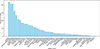 |
Figure 2. Number of labels per station used for training. |
The images were divided into three subsets, required for YOLOv5 training: 80% for the training set, 10% for validation, and 10% for testing. Since the dataset is relatively small, the distribution of images among these three subsets has an effect on the model performance (see Section 5.1). To address this, the training and validation subsets were randomly shuffled 10 times, while the test subset remained unchanged to allow consistent performance comparison across models. In addition, as the same events were seen by multiple telescopes, it was ensured that a given event did not appear in more than one subset. First, we verified that the test subset did not contain the same events as the training or validation subsets. Then, after each shuffle of the training and validation subsets, we verified that no events shared the same time and date between these subsets, and any similar event was assigned to the training subset. The average number of labels in each subset across all shuffles is summarized in Table 1.
Distribution of annotated burst labels across subsets, averaged over 10 random shuffles.
Four burst classes were considered: Type II, Type III, Type IV, and a Group of Type III defined as three or more Type III bursts in 4 minutes, facilitating labeling. The classes are approximately balanced with ∼400 images each, except Type IV with ∼130 images. Although this imbalance could potentially affect detection performance, later analysis shows that Type IV was the most accurately detected by YOLO, likely due to their distinctive shapes.
3.1 Data processing
The Flexible Image Transport System (FITS) files of radio bursts were retrieved from the e-CALLISTO database managed by the Institute for Data Science FHNW Brugg/Windisch, Switzerland (Monstein et al. 2023). Each spectrogram was rebinned to avoid frequency gaps and interpolated onto the same logarithmic frequency axis. The data were then normalized using the Z-score normalization also known as center and reduce, by subtracting from each frequency the mean and dividing by the standard deviation of each spectrogram. We evaluated several normalization methods, and Z-score normalization was retained for our base dataset. This normalization improved burst contrast and visually facilitated annotation as stations have different hardware and radio frequency interference environments. To account for the different frequency ranges of the telescopes, missing regions were filled with a dark background. The spectrograms were displayed in a grayscale colormap with an inverted log-scaled frequency axis from 450 MHz to 50 MHz and a 15 min time span. To reduce bias during training, all axis labels were removed. The resulting images were exported at a resolution of 640 × 640 pixels (see Sect. 5.2). Figure 3 illustrates the main steps of this processing.
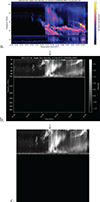 |
Figure 3. Main steps of spectrogram preprocessing: (a) default spectrogram on e-CALLISTO website, (b) rebinned and normalized on the same frequency axis for all spectrograms, (c) final resized image without axis labels. All three figures have the same x-axis ranges, covering a 15 min time span, while figures (b) and (c) have the same frequency range (y-axis) from 450 MHz to 50 MHz. |
3.2 Data augmentation
YOLOv5 applies data augmentation to the training dataset according to customizable hyperparameters. Given the small size of this dataset, the default low-hyperparameters were used (see Sect. 2.3). Additionally, a data augmentation step was applied to increase the size of the total dataset and improve the versatility of the model. The same preprocessing described in Section 3.1 was applied to all spectrograms, with one difference being the normalization. While the original dataset was normalized using the Z-score normalization, an alternative set of spectrograms was normalized by subtracting for each frequency the mean and dividing by the maximum. This alternative normalization produced visually more distinct images, with more background noise, compared to the Z-score normalized set, as shown in Figure 4. This augmentation exposed the model to images with strong background noise, allowing it to distinguish true bursts from noise. The burst labels remained unchanged, and the procedure doubled the number of training images.
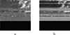 |
Figure 4. Example of data augmentation: excerpts of spectrograms from the MEXART telescope processed with (a) Z-score normalization and (b) normalization by subtracting the mean and dividing by the maximum value. The spectrogram covers a 15 min time span (x-axis) and a frequency range (y-axis) from 450 MHz to 50 MHz. |
4 Performance metrics
The performance of YOLOv5 was evaluated using standard object detection metrics (Everingham et al. 2010) that account for both the localization of bounding boxes and the correctness of class predictions. Localization accuracy was measured with the Intersection over Union (IoU), which quantifies the overlap between predicted and ground truth bounding boxes, defined as:
 (3)
(3)
where B p is the predicted bounding box and B g t the ground truth. A detection is considered correct if the IoU exceeds a chosen threshold.
For detection with correct localization, the class prediction was assessed using precision and recall. Precision measures the proportion of detected bursts that are correctly classified, and recall measures the proportion of actual bursts that are correctly detected. They are defined as:
 (4)
(4)
where T P, F P, and F N represent true positives, false positives, and false negatives, respectively. To summarize both incorrect classifications (low precision) and missed detections (low recall), the F1 score (Rainio et al. 2024) was used as the primary performance indicator, defined as:
 (5)
(5)
For completeness, we also computed the accuracy, which represents the proportion of correct predictions overall, including true negatives, TN as accuracy =  .
.
Another commonly used metric in object detection for evaluating matches between labeled and detected bounding boxes is the mean Average Precision (mAP). It is computed by first calculating the average precision for each class and then averaging these values. mAP is typically reported at an IoU of 0.5 (mAP@0.5), or averaged over multiple IoU thresholds. While the standard range is 0.5–0.95 in steps of 0.05 (mAP@0.5–0.95), here we report mAP@0.5–0.9 to match our threshold increments of 0.1. These values are given for the best-performing threshold combinations (see Sect. 6), although the configuration that generally maximizes performance occurs at a matching IoU of 0.2. mAP@0.5 and mAP@0.5–0.9 are provided for completeness and to facilitate comparison with other object detection models. For solar radio bursts, however, the best model is selected based on the F1 score, since avoiding missed bursts is prioritized over exact localization (see Sect. 7).
Finally, to evaluate whether differences in model performance were statistically meaningful, a paired t-test was applied. This approach was used because the same ten randomized image sets were kept unchanged across the different preprocessing methods (image size, data augmentation, and merging categories), allowing each model’s performance to be directly compared under matched conditions. For each shuffled dataset, the F1 score obtained under one condition was paired with the F1 score obtained under another condition, and the paired t-test evaluated whether the mean difference across these paired models is significantly different. Pairing the measurements reduces variability due to dataset differences, isolating the effect of the preprocessing strategies. The assumptions of the test are satisfied, as the comparisons are performed on naturally paired observations and the distribution of the performance differences was approximately normal for the ten runs. The paired t-test is expressed as:
 (6)
(6)
where  and s
d
are the mean difference and standard deviation of differences across n paired experiments. The statistical significance was determined at a p-value below 0.05.
and s
d
are the mean difference and standard deviation of differences across n paired experiments. The statistical significance was determined at a p-value below 0.05.
5 Performance comparison
The performance of YOLOv5 depends on several factors, including the distribution of images between training and validation subsets, the size of the images, the data augmentation, and the number of object categories. These variations are likely amplified by the relatively small size of our dataset. To investigate these effects, 10 randomly shuffled sets of images were generated and used to train our model. On the other hand, the test subset was kept identical across all shuffles, as described in Sect. 3. Training was performed using the default low-hyperparameters, a maximum of 300 epochs, and pretrained weights from the COCO dataset, which provide initial recognition of basic patterns or shapes that may appear in real spectrograms. Before applying the ensemble method, individual models were evaluated across thresholds, and Table 2 summarizes the best-performing configuration for each dataset, showing that the augmentation+merged dataset (see Sect. 5.5) achieved the highest F1 scores, which will later be compared with the ensemble results. The F1 score for each model on the test subset was recorded and will be analyzed in the following subsections.
Best performing single models configuration for each dataset. Bold values indicate the highest performance for each metric across all models.
5.1 Image distribution
Depending on how the images were distributed between the training and validation subsets, the performance on the test subset varied. The best-performing experiment achieved an F1 score of 0.627, while the worst-performing experiment achieved 0.505, resulting in a difference of 0.122. Across all runs, the mean F1 score was 0.558 with a standard deviation of 0.035. This means that the performance gap between the best and worst runs corresponds to about 3.5 times the standard deviation, indicating a substantial difference in performance.
Due to the small size of the dataset, the variability in the F1 scores is significantly different across the different random splits. Therefore, all 10 shuffled sets will be retained for the remaining performance tests, and the final results will be reported as the mean across these runs to provide a representative measure of the model performance.
5.2 Image size
The size of the training images also affects the model’s performance. Among the tested resolutions, images of size 640 × 640 pixels had the highest mean F1 score of 0.558 ± 0.035 across the 10 shuffled sets. By comparison, using images of 320 × 320 pixels and 1920 × 1920 pixels reduced the mean F1 scores to 0.521 ± 0.031 and 0.526 ± 0.032, respectively. A paired t-test confirmed that the difference between 320 pixels and 640 pixels is statistically significant, with a p-value of 0.0138. In contrast, the differences between 640 and 1920 pixels and between 320 and 1920 pixels were not statistically significant, with p-values of 0.100 and 0.780, respectively. The image size of 640 × 640 pixels was selected for the remaining performance analysis as its mean F1 score is higher than the 1920 × 1920 pixels, although the difference is not statistically significant, and it keeps computational cost low.
5.3 Augmentation
Data augmentation improves the performance of the YOLOv5 model. As described in Section 3.2, the dataset was doubled by applying modifications to the original normalization. The mean F1 score increased from 0.558 ± 0.035 without augmentation to 0.599 ± 0.025 with augmentation, with a paired t-test with a p-value of 0.005 and t-value of 3.69, indicating statistical significance. These results demonstrate that the model performs better when this additional normalization-based data augmentation is applied, which introduces more variability and background noise into the training data, reducing overfitting.
5.4 Merging Categories
Four categories were used for the original training; Type II, Type III, Type IV, and Group of a Type III. The definition of Group of Type III varies across the literature. For example, the National Oceanic and Atmospheric Administration (NOAA) defines the Group of Type III (also called Type VI) for their event reports as: “Series of Type III bursts over a period of 10 min or more, with no period longer than 30 minutes without activity”5.
In this study, we defined a Group of Type III bursts as three or more Type III events occurring within a 4-min interval. This definition was chosen because a spectrogram is only 15 min long and multiple Type III bursts often occur in succession, facilitating the labeling process. However, this distinction introduced some ambiguity for the model. Closely spaced bursts may be labeled as individual Type III events or as a group, depending on the context.
To reduce annotation-driven errors, the Type III and Group of Type III categories were merged. This resulted in a decrease in recall and an increase in precision. Closely spaced bursts that the model classified as a group were sometimes annotated as individual Type III events, producing false negatives and lowering recall, while fewer misclassifications of the background noise, as observed in the confusion matrix, improved precision. These predictions are not physically incorrect, as the distinction between the two categories is subjective. Importantly, merging only affects the category labels, as the original annotation rectangles were not changed. This reduces mislabeling between categories but does not change the number, position, or size of annotated bursts, so ambiguity for closely spaced events remains.
After merging, the F1 score increased from 0.558 ± 0.035 to 0.574 ± 0.022. However, the p-value does not indicate statistical significance with a p-value of 0.333.
5.5 Augmentation and Merging Categories
To test the combined effect of augmentation and category merging, the augmented+merged dataset was evaluated. This dataset applies data augmentation and merges Type III and Group of Type III bursts into a single class. The mean F1 score for this dataset was 0.583 ± 0.033, which is lower than the augmented-only dataset with 0.599 ± 0.025 but higher than the merged-only dataset with 0.574 ± 0.022 and the base dataset with 0.558 ± 0.035. A summary of the mean F1 scores across all datasets is shown in Figure 5.
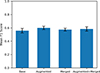 |
Figure 5. Mean F1 scores from all datasets evaluated on the test subset. Error bars represent standard deviation over 10 shuffled runs. |
Although the augmented-only dataset achieved the highest score, none of the differences between the new datasets were statistically significant, with all p-values greater than 0.05. Therefore, all four datasets were retained for the following ensemble method experiments, with the base dataset included as a reference.
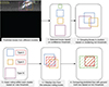 |
Figure 6. Schematic example of ensemble process on a spectrogram segment: overlapping predictions from multiple YOLOv5 models are combined to produce final classes and bounding boxes. The bounding boxes are illustrative only. |
6 Ensemble method
To improve predictive performance, outputs from multiple YOLOv5-based models were combined using ensemble methods. Three approaches were tested: hard voting, soft voting, and Weighted Box Fusion (WBF) (Saponara and Elhanashi 2022). For each dataset (base, merged, augmentation, and augmented+merged), the same ten sets of images were used for training as explained in Section 5. Ensemble prediction was performed with each dataset, using only models trained on the respective dataset. Figure 6 schematically illustrates the main steps of the ensemble method. Step 1: Bounding boxes must exceed a confidence threshold, which is provided by the YOLO output, to be considered for step 2. In the example, the yellow rectangle on the left does not pass this threshold and is therefore discarded. Step 2: The remaining bounding boxes are grouped based on a selected clustering IoU threshold, such that overlapping boxes are considered to represent the same object. Step 3: Within each cluster, the ensemble method determines the final class based on a vote or confidence level threshold, and step 3.1: The final bounding box is computed by taking the median of each of the four coordinates (x min, y min, x max, y max) separately across all boxes in the cluster. Step 4: The final predicted bounding box, shown in red, is then compared with the ground-truth-labeled burst, in green, for evaluation. These steps correspond directly to the tunable threshold parameters listed below.
-
1.
Minimum confidence threshold: Minimum confidence for a predicted box to be considered in the ensemble prediction, varied from 0.2 to 0.9.
-
2.
Clustering IoU threshold: Minimum IoU to define a cluster of overlapping boxes, varied from 0.2 to 0.9.
-
3.
Final class confidence threshold: Minimum confidence value required to assign a class within a cluster, or the minimum number of votes, varied from 0.2–0.9 or 2–9 votes.
-
4.
Matching IoU threshold: Minimum IoU value above which a predicted box is considered a true positive, varied from 0.2 to 0.9.
False positives, which are predicted boxes that do not correspond to any ground truth, and false negatives, which are ground truth boxes without a matching prediction, were also computed for each evaluation.
The ensemble evaluation was performed on a separate test set of 205 images collected from e-CALLISTO from February to July 2024, processed as described in Sect. 3.1. This set included 67 Type II, 56 Type III, 71 Type IV, 51 Group of Type III radio bursts, and 29 background images. Using an independent dataset ensures an unbiased assessment of the ensemble’s performance, confirming that any improvements reflect the method itself rather than overfitting to previously seen data.
6.1 Single Models
Before applying the ensemble method, the performance of individual models was evaluated across the minimum confidence threshold and the final matching IoU threshold. This process generated 640 files per dataset, each containing the predictions for the 10 shuffled sets. Table 2 summarizes the best-performing configuration for each dataset, where the highest mAP@0.5 does not necessarily correspond to the optimal balance between precision and recall. Among all models, model number 3 from the augmentation-merged dataset achieved the highest F1 score of 0.704, while the top five configurations from this dataset averaged 0.693 ± 0.008, as shown in Figure 7. A paired t-test confirmed that the average F1 score of the augmentation-merged dataset was statistically significantly higher than those of the three other datasets.
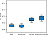 |
Figure 7. Box plot of F1 score of the best five single models per dataset. The central line represents the median, the box indicates the interquartile range (IQR), and the whiskers extend to the most extreme values within 1.5× IQR. |
These models will be used for comparison with the ensemble methods to evaluate whether the ensemble outperforms the individual model approach.
6.2 Hard Voting
Hard voting combines predictions by grouping bounding boxes and assigning the final class based on majority vote. Three parameters were varied: clustering IoU, final class vote threshold (2–9), and matching IoU, producing 512 parameter combinations per dataset.
For each cluster, a class label was assigned if the number of agreeing models met the vote threshold. The final bounding box coordinates were defined as the median of the contributing boxes. Table 3 summarizes the best performing configuration for each dataset. Overall, both the F1 score and mAP metrics improved compared to single models. Among them, the augmentation-merged dataset achieved the highest F1 score at 0.728, which is higher than the best-performing single model.
Best performing hard voting configuration for each dataset.
When considering the best five runs for each dataset, the difference between the datasets in the mean F1 score was statistically significant, with all p-values below 0.05. The augmented+merged dataset has the highest mean F1 score of 0.721 ± 0.004, as shown in Figure 8, with a p-value of 0.00008 and t-value of 16.3 when compared to the single base models.
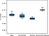 |
Figure 8. Box plot of F1 score of the top five hard voting runs per dataset. |
Compared with the best-performing single models, hard voting consistently improved the F1 score across all datasets, demonstrating the benefit of combining model predictions rather than relying on individual outputs.
6.3 Soft Voting
Soft voting is an ensemble method where predictions from multiple models are combined by averaging their confidence scores. In this study, four parameters were varied: minimum confidence threshold, clustering IoU threshold, final class confidence threshold (0.2–0.9), and matching IoU threshold. This setup produced 4096 parameter combinations per dataset.
Predictions from the ten models were first filtered by a minimum confidence threshold, then clustered using the clustering IoU threshold. Each cluster’s class was assigned based on the highest mean confidence, and its final box was defined by the mean coordinates. Table 4 presents the best performing configurations for each dataset. Although soft voting achieved mAP values comparable to single models, its F1 score was consistently lower. Among them, the merged dataset achieved the highest F1 score of 0.685. However, soft voting did not outperform the individual model predictions, with the F1 score consistently lower than the best individual model.
Best performing soft voting configuration for each dataset.
6.4 Weighted Box Fusion
Weighted Box Fusion (WBF) was also evaluated as an ensemble method. WBF first applies weights at the model level, giving more influence to some models in the final prediction. Bounding boxes from all models were grouped based on the clustering IoU threshold, and final coordinates were calculated as a confidence-weighted mean of the overlapping boxes. The WBF was done using the implementation provided by Solovyev et al. (2021).
As in soft voting experiments, four parameters were varied: minimum confidence threshold, clustering IoU threshold, final class confidence threshold (0.2–0.9), and matching IoU threshold. This produced 4096 parameter combinations per dataset. The best unweighted configuration for each dataset is summarized in Table 5.
Best performing Weighted Box Fusion configuration for each dataset with no weight assigned.
WBF requires weights to be assigned in order to perform as intended, as the unweighted version performed worse than both hard and soft voting. To determine these optimal weights, the best-performing unweighted parameter configuration for each dataset was first identified (Table 5), after which models were ranked by their individual F1 scores and assigned weights from 10 (best) to 1 (worst). An exponent of 0.5 was applied to the rank values (wi = ri0.5) to reduce the disparity between models, ensuring more balanced contributions since their performances are relatively similar. Table 6 summarizes the best results obtained with this weighting scheme, where F1 score and mAP values both agreed on the best-performing model. Among the weighted configurations, the augmented+merged dataset achieved the highest F1 score of 0.738.
Best performing Weighted Box Fusion configuration for each dataset with weights.
When averaging across the best five configurations for each dataset, the augmented+merged dataset achieved the highest F1 score of 0.738 ± 0.004. This improvement was statistically significant compared to the other datasets, with a p-value of 0.000008 and a t-value of 29.2 when compared to the single base dataset. Furthermore, the augmented+merged dataset under WBF outperformed both single model predictions and hard voting, making it the most effective method tested in this study (t = 10.7, p = 0.0004 between hard voting and Weighted Box Fusion).
7 Discussion
This study identifies several factors influencing the performance of the YOLOv5-based model for automated detection of solar radio bursts across the e-CALLISTO network. Variability across different training and validation splits illustrates the challenges of working with a limited dataset. This variability motivated the exploration of ensemble methods as a strategy to exploit these differences to improve predictive performance.
The choice of image resolution had an influence on the performance. Optimal results were obtained with a moderate image resolution of 640 × 640 pixels. This resolution preserves structural details essential for burst classification, particularly Type III events, while avoiding excessive noise amplification that could increase false positives. Burst features may become more or less distinguishable depending on image resolution (Saponara and Elhanashi 2022). At lower resolutions, fine details may be lost, leading to false negatives (e.g Type III are not detected), while higher resolutions can introduce noise, increasing false positives (background misclassified as Type III). These effects were also reflected in the confusion matrices produced by YOLOv5, where misclassifications increased at both lower and higher resolutions.
Normalization-based data augmentation contributed to improved generalization by increasing variability in the training set. This augmentation likely helped the model reduce overfitting and increase performance across telescopes with different instrumental characteristics.
Merging Type III and Group of Type III burst categories increased precision but decreased recall. By treating closely spaced bursts as a single event, the model reduces false positives, but individual bursts are undercounted, producing more false negatives. Frequently, the model predicts a single Group of Type III event where multiple individual Type III bursts are annotated, lowering recall, although this is not physically incorrect. The augmented+merged dataset combines both data augmentation and category merging strategies, providing a balance between precision and generalization.
Ensemble methods further improved performance. Hard voting and Weighted Box Fusion both consistently outperformed single model predictions, with the augmented+merged dataset achieving the highest F1 scores. Weighted Box Fusion, in particular, reached a mean F1 of 0.738 ± 0.004, significantly higher than hard voting (0.721 ± 0.004), as shown in Figure 9. In contrast, soft voting underperformed compared to individual models, and the reasons for this have yet to be determined.
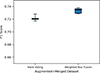 |
Figure 9. Boxplot of the top five F1 scores on the augmented+merged dataset for hard voting and WBF. |
Visual inspection of spectrograms confirms that what the model detects as a single continuous structure is sometimes annotated as multiple individual bursts. Figure 10 shows an example from the MEXICO-LANCE-A instrument. Some of the wave-like patterns visible in the background are likely interferences from power supplies of equipment in the vicinity of the antenna. The blue rectangles indicate ground truth annotations, and the orange rectangles show predictions from the best Weighted Box Fusion model. The model correctly identifies the general location of the Type III bursts, but sometimes merges what are annotated as multiple Type III bursts into a single detection. This highlights a limitation on the labeling rather than the detection capability of the model itself.
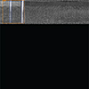 |
Figure 10. Spectrogram from the MEXICO-LANCE-A station, showing Type III bursts. The blue rectangles indicate ground truth, orange rectangle shows prediction by the best Weighted Box Fusion model. The spectrogram covers a 15 min time span (x-axis) and a frequency range (y-axis) from 450 MHz to 50 MHz. |
Additionally, individual Type III bursts are often missed because they look like the background noise. Variability in the background between different instruments exacerbates this issue, making subtle bursts harder to detect consistently. For example, in the spectrogram from the INDIA-OOTY station (Fig. 11), the model successfully detects a group of Type III bursts, but three faint single Type III bursts are not detected due to their low contrast against the background.
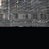 |
Figure 11. Spectrogram from the INDIA-OOTY station, showing Type III bursts. Blue rectangles indicate ground truth,orange rectangles show predictions by the best Weighted Box Fusion model. The spectrogram covers a 15 min time span (x-axis) and a frequency range (y-axis) from 450 MHz to 50 MHz. |
Table 7 summarizes the per-class performance of the best Weighted Box Fusion model, highlighting lower recall for Type III / Group of Type III bursts due to annotation ambiguities and subtle events that resemble background noise.
Performance metrics per class of the best Weighted Box Fusion model.
For Type II and Type IV bursts, the model achieved higher precision and recall compared to Type III/Group of Type III events. However, the remaining false positives and false negatives for these classes are largely due to annotation inconsistencies rather than actual misclassifications. The model’s predictions are physically reasonable but sometimes differ from the ground truth due to subjective labeling choices, such as whether an extended bursts is annotated as a single event (Fig. 12) or split into multiple parts (Fig. 13). Importantly, the model shows little confusion between classes, distinguishing Type III/Group of Type III, Type II, and Type IV. Using longer-duration spectrograms might reduce annotation ambiguity by providing the full extent of each event.
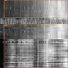 |
Figure 12. Spectrogram from the AUSTRIA-OE3FLB station showing a Type IV burst. Blue rectangles indicate ground truth, orange rectangles show predictions by the best Weighted Box Fusion model. The spectrogram covers a 15 min time span (x-axis) and a frequency range (y-axis) from 450 MHz to 50 MHz. |
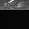 |
Figure 13. Spectrogram from the BIR station showing a Type II burst. Blue rectangles indicate ground truth, orange rectangles show predictions by the best Weighted Box Fusion model. The spectrogram covers a 15 min time span (x-axis) and a frequency range (y-axis) from 450 MHz to 50 MHz. |
Model selection based on F1 score balances precision and recall, capturing both correct detections and missed events. While mAP emphasizes precision and localization accuracy, which can be misleading for ensemble methods with averaged bounding boxes. Selecting by mAP@0.5 can reduce recall as averaging coordinates can shift or enlarge boxes, making exact localization less precise. In our results, single models and hard voting would have lower recall if chosen by mAP@0.5, while soft voting would increase recall, but it performed worse overall. For Weighted Box Fusion, F1 score and mAP metrics agreed on the highest-performing model. Lower IoU thresholds, such as 0.2, help account for this effect, prioritizing detection over exact box alignment. F1 provides a more reliable criterion for selecting the best-performing model with an ensemble model, with mAP values serving as a reference for localization accuracy.
Overall, this study emphasizes that model performance in this context is not only due to the architecture and training strategies but also to the dataset characteristics, annotation practices, and the variability of multi-instrument observations.
8 Conclusions
In this work, it has been demonstrated that YOLOv5, combined with ensemble methods, can effectively detect and classify solar radio bursts across the e-CALLISTO network. The experiments showed that several factors influence model performance, including image resolution, data augmentation, and category definition. A moderate resolution of 640 × 640 pixels was found to preserve burst morphology while minimizing false positives, and data augmentation improved generalization across telescopes with different instrumental characteristics.
Merging Type III and Group of Type III bursts into a single category increased precision while decreasing recall, reducing false positives but undercounting individual bursts. The augmented+merged dataset, combining data augmentation and category merging, provided a balanced approach that improved overall performance. In addition, the ensemble methods further improved the detection performance. Hard voting outperformed individual model predictions, while Weighted Box Fusion achieved the highest mean F1 score of 0.738 ± 0.004, significantly better than hard voting. In contrast, Soft voting did not outperform single models,
A consistent limitation remains the relatively low recall for Type III and Group of Type III, primarily due to annotation ambiguities and the difficulty in detecting single bursts in the background noise. Visual inspection confirms that some apparent false negatives are rather due to labeling inconsistencies than to truly undetected bursts. While multiple stations observe the Sun simultaneously, only large events appear across most instruments; smaller bursts are usually seen by one or two stations. This variability in detection across stations limits the ability to improve recall by combining observations, and the model performs well on strong events but struggles with faint bursts.
Future improvements could include using a sliding window of spectrograms to capture full events such as Type II and Type IV bursts that often last hours. Additionally, redefining the annotation for Type III and the group of Type III to reduce ambiguity between these categories. A critical step would be to evaluate the method’s generalization by testing it on spectrograms from telescopes that were not included in the training or validation subset, which would show the ability of the models to handle unseen instrument characteristics.
Overall, this study showed that YOLOv5, combined with ensemble methods and carefully designed data preprocessing strategies, can reliably detect and classify solar radio bursts across the e-CALLISTO network. The results emphasize that model performance is not solely determined by the architecture but also by dataset characteristics, annotation practices, and multi-instrument variability. The findings provide a foundation for future automated monitoring of solar radio activity and support improved consistency in burst detection. The finalized model is now performing and publicly available for the HUMAIN CALLISTO station at the Solar Influence Data Analyses Center (SIDC)6.
Acknowledgments
We are grateful to the e-CALLISTO network and its instrument operators for providing open access solar radio spectrograms. We also acknowledge the work of Andreas Wassmer for producing the burst lists used for training and validation. The editor thanks Javier Bussons and an anonymous reviewer for their assistance in evaluating this paper.
Funding
This work received financial support from the Belgian Federal Science Policy Office (BELSPO) in the framework of the Brain-be program under contract number B2/202/P1/DELPHI and in the framework of the PRODEX Program of the European Space Agency (ESA) under contract number 4000147286. Finally, Philippe Vong was supported by a PhD grant awarded by the Royal Observatory of Belgium.
Conflict of interest
The authors declare no conflict of interest.
Data availability statement
The spectrograms used in this study were obtained from the e-CALLISTO network available at https://soleil.i4ds.ch/solarradio/.
The burst lists compiled by Andreas Wassmer and used to categorize bursts were derived from the catalogs available at https://soleil.i4ds.ch/solarradio/data/BurstLists/2010-yyyy_Monstein/.
The spectrograms and corresponding labels used for model training are publicly available on Zenodo at https://doi.org/10.5281/zenodo.18701288.
The YOLOv5 model implementation used in this work is publicly available from Ultralytics at https://github.com/ultralytics/yolov5.
References
- Afandi N, Sabri N, Umar R, Monstein C. 2020. Burst-Finder: burst recognition for E-CALLISTO spectra. Indian J Phys 94(7): 947–957. https://doi.org/10.1007/s12648-019-01551-2. [Google Scholar]
- Benz AO, Monstein C, Meyer H, Manoharan PK, Ramesh R, et al. 2009. A world-wide net of solar radio spectrometers: e-CALLISTO. Earth Moon Planets 104(1): 277–285. https://doi.org/10.1007/s11038-008-9267-6. [NASA ADS] [CrossRef] [Google Scholar]
- Bochkovskiy A, Wang C-Y, Liao H-YM. 2020. YOLOv4: Optimal speed and accuracy of object detection. PrearXiv https://arxiv.org/abs/2004.10934. [Google Scholar]
- Bussons Gordo J, Fernández Ruiz M, Prieto Mateo M, Alvarado Díaz J, Chávez de la O F, et al. 2023. Automatic burst detection in solar radio spectrograms using deep learning: deARCE Method. Sol Phys 298: 82. https://doi.org/10.1007/s11207-023-02171-0. [Google Scholar]
- Deng J, Yuan G, Zhou H, Wu H, Tan C. 2024. Real-time automated detection of multi-category solar radio bursts. Astrophys Space Sci 369(10): 99. https://doi.org/10.1007/s10509-024-04364-w. [Google Scholar]
- Diwan T, Ani A, Tembhurne J. 2022. Object detection using YOLO: challenges, architectural successors, datasets and applications. Multimedia Tools Appl 82: 9243–9275. https://doi.org/10.1007/s11042-022-13644-y. [Google Scholar]
- Doherty J, Gardiner B, Kerr E, Siddique N, Manvi SS. 2022. Comparative study of activation functions and their impact on the YOLOv5 object detection odel. In: Pattern recognition and artificial intelligence, El Yacoubi M, Granger E, Yuen PC, Pal U, Vincent N (Eds.), Springer International Publishing, Cham. pp. 40–52. ISBN 978-3-031-09282-4. https://doi.org/10.1007/978-3-031-09282-4_4. [Google Scholar]
- Everingham M, Van Gool L, Williams CK, Winn J, Zisserman A. 2010. The pascal visual object classes (voc) challenge. Int J Comput Vision 88(2): 303–338. https://doi.org/10.1007/s11263-009-0275-4. [Google Scholar]
- He H, Yuan G, Zhou H, Tan C, Guo S. 2023. Solar radio burst detection based on the MobileViT-SSDLite lightweight model. Astrophys J Suppl Ser 269(2): 51. https://doi.org/10.3847/1538-4365/ad036c. [Google Scholar]
- Khanam R, Hussain M. 2024. What is YOLOv5: A deep look into the internal features of the popular object detector. PrearXiv https://arxiv.org/abs/2407.20892. [Google Scholar]
- Lin T-Y, Maire M, Belongie S, Bourdev L, Girshick R, et al. 2015. Microsoft COCO: Common Objects in Context. https://arxiv.org/abs/1405.0312. [Google Scholar]
- Lobzin VV, Cairns IH, Robinson PA, Steward G, Patterson G. 2009. Automatic recognition of type III solar radio bursts: automated radio burst identification system method and first observations. Space Weather 7: 4. https://doi.org/10.1029/2008SW000425. [Google Scholar]
- Lobzin VV, Cairns IH, Robinson PA, Steward G, Patterson G. 2010. Automatic recognition of coronal type II radio bursts: the automated radio burst identification system method and first observations. Astrophys J Lett 710(1): L58. https://ui.adsabs.harvard.edu/link_gateway/2010ApJ...710L..58L/doi:10.1088/2041-8205/710/1/L58. [Google Scholar]
- Monstein C, Csillaghy A, Benz AO. 2023. CALLISTO Quicklook solar spectrogram plots. Accessed: 2025-08-18. https://doi.org/10.48322/WY0B-TQ35. https://spase-metadata.org/ISWI/DisplayData/Callisto/FAS/PT15M. [Google Scholar]
- Pick M, Vilmer N. 2008. Sixty-five years of solar radioastronomy: Flares, coronal mass ejections and Sun-Earth connection. Astron Astrophys Rev 16: 1–153. https://doi.org/10.1007/s00159-008-0013-x. [CrossRef] [Google Scholar]
- Rainio O, Teuho J, Klén R. 2024. Evaluation metrics and statistical tests for machine learning. Sci Rep 14(1): 6086. https://doi.org/10.1038/s41598-024-56706-x. [Google Scholar]
- Redmon J, Divvala S, Girshick R, Farhadi A. 2016. You only look once: Unified, real-time object detection. https://arxiv.org/abs/1506.02640. [Google Scholar]
- Saponara S, Elhanashi A. 2022. Impact of image resizing on deep learning detectors for training time and model performance. In: Applications in electronics pervading industry, environment and society, Saponara S, De Gloria A (Eds.), Springer International Publishing, Cham., ISBN 978-3-030-95498-7. https://doi.org/10.1007/978-3-030-95498-7_2. [Google Scholar]
- Solovyev R, Wang W, Gabruseva T. 2021. Weighted boxes fusion: Ensembling boxes from different object detection models. Image Vision Comput 107: 1–6. https://doi.org/10.48550/arXiv.1910.13302. [Google Scholar]
- Wang M, Yuan G, He H, Tan C, Wu H, Zhou H. 2025. Multi-category solar radio burst detection based on task-aligned one-stage object detection model. Astrophys Space Sci 370(3): 23. https://doi.org/10.48550/arXiv.2503.16483. [Google Scholar]
- White SM. 2024. Solar radio bursts and space weather. https://arxiv.org/abs/2405.00959. [Google Scholar]
- Zhang W, Wang B, Wu Z, Chen Y, Yan F. 2024. Identification and extraction of type II and III radio bursts based on YOLOv7. Astron Astrophys 683: A90. https://doi.org/10.1051/0004-6361/202348026. [Google Scholar]
Astrodoncel Data Center, Universidad de Alcalá : https://astrodoncel.uah.es/dashboard/statistics.php. Accessed on 2025-08-29.
Ultralytics YOLOv5 repository https://github.com/ultralytics/yolov5
List of bursts made by Andreas Wassmer: https://soleil.i4ds.ch/solarradio/data/Bursts/
Labelme repository: https://github.com/zhong110020/labelme Accessed on 2025-08-18.
Finalized Model running on SIDC: https://www.sidc.be/humain/callisto-latest-ai-burst-class
Cite this article as: Tassan-Din E, Gunessee AA, Vong P, Marqué C, Martínez Picar A, Monstein C. 2024. Automated detection and classification of solar radio bursts in CALLISTO spectrograms using deep-learning YOLOv5 model and ensemble methods. J. Space Weather Space Clim. 16, 16. https://doi.org/10.1051/swsc/2026014.
All Tables
Distribution of annotated burst labels across subsets, averaged over 10 random shuffles.
Best performing single models configuration for each dataset. Bold values indicate the highest performance for each metric across all models.
Best performing Weighted Box Fusion configuration for each dataset with no weight assigned.
Best performing Weighted Box Fusion configuration for each dataset with weights.
All Figures
|
Figure 1. Architecture of the You Only Look Once (YOLO) object-detection model. Adapted from Bochkovskiy et al. (2020). |
| In the text | |
|
Figure 2. Number of labels per station used for training. |
| In the text | |
|
Figure 3. Main steps of spectrogram preprocessing: (a) default spectrogram on e-CALLISTO website, (b) rebinned and normalized on the same frequency axis for all spectrograms, (c) final resized image without axis labels. All three figures have the same x-axis ranges, covering a 15 min time span, while figures (b) and (c) have the same frequency range (y-axis) from 450 MHz to 50 MHz. |
| In the text | |
|
Figure 4. Example of data augmentation: excerpts of spectrograms from the MEXART telescope processed with (a) Z-score normalization and (b) normalization by subtracting the mean and dividing by the maximum value. The spectrogram covers a 15 min time span (x-axis) and a frequency range (y-axis) from 450 MHz to 50 MHz. |
| In the text | |
|
Figure 5. Mean F1 scores from all datasets evaluated on the test subset. Error bars represent standard deviation over 10 shuffled runs. |
| In the text | |
|
Figure 6. Schematic example of ensemble process on a spectrogram segment: overlapping predictions from multiple YOLOv5 models are combined to produce final classes and bounding boxes. The bounding boxes are illustrative only. |
| In the text | |
|
Figure 7. Box plot of F1 score of the best five single models per dataset. The central line represents the median, the box indicates the interquartile range (IQR), and the whiskers extend to the most extreme values within 1.5× IQR. |
| In the text | |
|
Figure 8. Box plot of F1 score of the top five hard voting runs per dataset. |
| In the text | |
|
Figure 9. Boxplot of the top five F1 scores on the augmented+merged dataset for hard voting and WBF. |
| In the text | |
|
Figure 10. Spectrogram from the MEXICO-LANCE-A station, showing Type III bursts. The blue rectangles indicate ground truth, orange rectangle shows prediction by the best Weighted Box Fusion model. The spectrogram covers a 15 min time span (x-axis) and a frequency range (y-axis) from 450 MHz to 50 MHz. |
| In the text | |
|
Figure 11. Spectrogram from the INDIA-OOTY station, showing Type III bursts. Blue rectangles indicate ground truth,orange rectangles show predictions by the best Weighted Box Fusion model. The spectrogram covers a 15 min time span (x-axis) and a frequency range (y-axis) from 450 MHz to 50 MHz. |
| In the text | |
|
Figure 12. Spectrogram from the AUSTRIA-OE3FLB station showing a Type IV burst. Blue rectangles indicate ground truth, orange rectangles show predictions by the best Weighted Box Fusion model. The spectrogram covers a 15 min time span (x-axis) and a frequency range (y-axis) from 450 MHz to 50 MHz. |
| In the text | |
|
Figure 13. Spectrogram from the BIR station showing a Type II burst. Blue rectangles indicate ground truth, orange rectangles show predictions by the best Weighted Box Fusion model. The spectrogram covers a 15 min time span (x-axis) and a frequency range (y-axis) from 450 MHz to 50 MHz. |
| In the text | |
Current usage metrics show cumulative count of Article Views (full-text article views including HTML views, PDF and ePub downloads, according to the available data) and Abstracts Views on Vision4Press platform.
Data correspond to usage on the plateform after 2015. The current usage metrics is available 48-96 hours after online publication and is updated daily on week days.
Initial download of the metrics may take a while.