| Issue |
J. Space Weather Space Clim.
Volume 16, 2026
|
|
|---|---|---|
| Article Number | 17 | |
| Number of page(s) | 20 | |
| DOI | https://doi.org/10.1051/swsc/2026008 | |
| Published online | 19 May 2026 | |
Research Article
Global IsUG index maps for tracking ionospheric variability: a case study of the 4–5 November 2023 geomagnetic storm
1
Department of Earth and Environmental Sciences, Ludwig Maximilian University of Munich, Munich, Germany
2
GFZ Helmholtz Centre for Geosciences, Potsdam, Germany
3
National Institute of Geophysics and Volcanology (INGV), Rome, Italy
4
University of Salento, Lecce, Italy
5
Departament of Mathematics, Faculty of Sciences, Universitat Autònoma de Barcelona, E-08193 Barcelona, Spain
6
Observatori de l’Ebre (OE), Univ. Ramon Llull - CSIC, E-43520 Roquetes, Spain
7
College of Geography and Environmental Science, Henan University, Kaifeng, PR China
8
Universitat Politècnica de Catalunya (UPC-IonSAT), Barcelona, Spain
9
Institut d’Estudis Espacials de Catalunya (IEEC), Barcelona, Spain
* Corresponding author: This email address is being protected from spambots. You need JavaScript enabled to view it.
; This email address is being protected from spambots. You need JavaScript enabled to view it.
; This email address is being protected from spambots. You need JavaScript enabled to view it.
Received:
20
August
2025
Accepted:
27
February
2026
Abstract
In this study, we analyze ionospheric and thermospheric changes during a composite geomagnetic storm on 4–5 November 2023 with two activity periods. On 4 November, the corotating interaction region (CIR) compression resulted in moderate activity (SYM-H = −60 nT), while on 5 November the arrival of two Coronal Mass Ejections (CMEs) embedded into the ongoing CIR caused intense geomagnetic disturbances (SYM-H = −188 nT). Using global observations of vertical total electron content (VTEC) from the Universitat Politècnica de Catalunya (UPC) Global Ionosphere Maps (GIMs) and the normalized Ionospheric storm scale from UPC GIMs (IsUG) storm-time index, we examine ionospheric anomalies during these events. The IsUG index reveals that both events began with positive VTEC changes, but their delayed responses differed significantly. During the 4 November event, the negative phase did not develop, while the 5 November storm produced severe negative VTEC anomalies. Using complementary satellite observations of thermospheric composition, temperature and density, along with ionosonde-derived large-scale traveling ionospheric disturbances (LSTIDs) velocities, we show that these contrasting responses were caused by differences in thermospheric heating and composition. On 4 November, high-latitude heating was weak, while in the 5 November storm it was significant and led to the development of global disturbance winds and strong O/N2 decreases, causing severe negative VTEC anomalies. Despite the complicated morphology, the IsUG index could track these dynamics in agreement with the underlying physical processes, and can be used for monitoring of complex ionospheric storms.
Key words: Ionospheric indices / Geomagnetic storms / Space weather
© A. Smirnov et al., Published by EDP Sciences 2026
 This is an Open Access article distributed under the terms of the Creative Commons Attribution License (https://creativecommons.org/licenses/by/4.0), which permits unrestricted use, distribution, and reproduction in any medium, provided the original work is properly cited.
1 Introduction
During geomagnetic storms, large amounts of energy and momentum are deposited into the high-latitude ionosphere, causing rapid and dramatic changes in the ionosphere-thermosphere (IT) system (Buonsanto, 1999; Mendillo, 2006; Prölss, 2008; Kelley et al., 2011). These changes lead to fast and often unpredictable fluctuations in electron density that can adversely affect various technological systems. In particular, storm-time ionospheric variations frequently degrade the Global Navigation Satellite Systems (GNSS) accuracy and cause blackouts of high-frequency (HF) and satellite communications (e.g. Liu et al., 2021). In order to mitigate these hazardous effects, it is important to study the influence of geomagnetic storms on the ionosphere-thermosphere system and improve our capabilities of monitoring these events.
One of the ways to monitor storm-time changes in different domains of the near-Earth space environment is by using activity indices. For instance, the geomagnetic Kp index reflects the magnetic field disturbances on a planetary scale (e.g. Matzka et al., 2021). Other widely used proxies include the Disturbance storm time (Dst) index, which quantifies ring current strength, and auroral indices such as the Auroral Electrojet (AE) index (Mayaud, 1980). Each of these indices provides a one-dimensional activity proxy. However, ionospheric morphology during storms depends to a large extent on solar activity phase, season, local time and location. This additional complexity makes finding a unified ionospheric index challenging, and multiple storm-time proxies have been proposed over the years. Notable approaches include the global planetary ionospheric index WP (Gulyaeva & Stanislawska, 2008), a disturbance ionospheric index (DIX) based on dual-frequency GNSS carrier phase measurements (Jakowski et al., 2012) and its modifications (Wilken et al., 2018), ionosonde-based indices (Bremer et al., 2006), and those combining ionosonde and Vertical Total Electron Content (VTEC) observations (Nishioka et al., 2017), as well as recently developed disturbance indices based on the temporal VTEC changes (Nykiel et al., 2024a).
Recently, Liu et al. (2021) proposed global maps of ionospheric storm-time indices IsUG, derived from the VTEC maps produced by Universitat Politècnica de Catalunya (UPC-IonSAT research group). IsUG represents local VTEC anomalies with respect to the 27-day averages in the respective bins of latitude and local time, further standardized across seasons and solar cycle phases. To assess the ability of IsUG maps to capture storm-time ionospheric variability, it is important to analyze the features they depict in relation to known physical drivers. In particular, the ionospheric behavior during storms can be classified into the positive and negative phases, which correspond to the enhancements or depletions of VTEC, respectively (Appleton & Ingram, 1935; Berkner et al., 1939; Rishbeth, 1998; Mendillo, 2006). Although the precise sequence of events and the interplay of different drivers are unique for each storm, it is generally possible to distinguish between drivers leading to immediate storm-time effects, such as fast modifications of the electrodynamics, and delayed effects due to changes in the thermospheric composition and global circulation patterns (Fuller-Rowell et al., 1994, 1996; Rishbeth, 1998; Förster & Jakowski, 2000; Mendillo, 2006; Prölss, 2011).
Fast initial changes in the ionosphere-thermosphere system during geomagnetic storms are caused by the development of the so-called prompt penetration electric fields (PPEFs) (Nishida, 1968; Kikuchi et al., 1996, 2008, 2010; Huang et al., 2007). They occur due to rapid changes in the magnetospheric convection pattern that allows it to expand down to equatorial latitudes almost instantaneously and cause changes in the plasma distribution within around 1–2 h. The resulting PPEF is usually directed eastward on the dayside and westward on the nightside, altering the E × B drift directions in the equatorial ionosphere (e.g. Fejer & Scherliess, 1997; Fejer et al., 2008; Xiong et al., 2016). During the day, PPEFs generally increase the upward E × B velocity and lead to an intensification of the equatorial ionization anomaly (EIA). During particularly strong events, PPEFs can produce the so-called superfountain effect which corresponds to poleward extension of the EIA crests and higher electron densities at low- and mid-latitudes (e.g. Mannucci et al., 2005; Tsurutani et al., 2007; Venkatesh et al., 2019; Rout et al., 2025).
Prompt penetration electric fields do not remain active for longer than a few hours, and the later storm-time changes in the IT system are generally attributed to changes in the atmospheric composition and global circulation patterns (Fuller-Rowell et al., 1994, 1996; Rishbeth, 1998; Prölss, 2008, 2011). Storm-time high-latitude heating enhances neutral temperatures, establishing meridional pressure gradients that create equatorward winds and a change of global circulation that can persist for over a day. In addition, the impulsive nature of energy input at high latitudes launches atmospheric gravity waves (AGWs), which can take 4–6 h to reach the equator (Blanc & Richmond, 1980; Richmond et al., 2003; Xiong et al., 2015). The combination of these processes has two important implications: (1) it creates a disturbance dynamo electric field (DDEF) that leads to downward E × B drifts at the equator during daytime, suppressing the EIA formation and contributing to negative storm-time effects, and (2) upwelling of the molecular-rich air that reduces the O/N2 ratios and also leads to negative storm-time anomalies in VTEC (Astafyeva et al., 2015; Nava et al., 2016). A further manifestation of these storm-time winds is the generation of Large-Scale Traveling Ionospheric Disturbances (LSTIDs), which present wave-like plasma density fluctuations propagating equatorward with periods longer than 1 h, velocities over 300 m/s and wavelengths between 1000 and 3000 km (e.g. Prölss & Ocko, 2000; Hernández-Pajares et al., 2012; Tsagouri et al., 2023; Nykiel et al., 2024b). LSTID velocities can be tracked by means of both the GNSS receivers and ionosondes and can serve as a proxy for the development of storm-time neutral winds and their directions (Bowman, 1965; Maeda & Handa, 1980; Tedd & Morgan, 1985; Altadill et al., 2020).
In this study, we analyze a composite geomagnetic storm on 4–5 November 2023 in order to assess the ability of the IsUG index to track the storm-time variability of the ionosphere and to evaluate its consistency with physical processes in the ionosphere-thermosphere system. This storm had two activity periods, with moderate disturbances on 4 November and a period of strong geomagnetic activity a day later. These events corresponded to complex heliospheric morphology and resulted in vastly different ionospheric responses, with mostly positive VTEC anomalies on 4 November and severe negative changes following the 5 November event. Furthermore, the 4–5 November events prompted a rare and severe degradation of the Approach with Vertical Guidance-I (APV-I) availability of the European Geostationary Navigation Overlay Service (EGNOS). APV-I defines the safety margins indicating how much error is acceptable in horizontal and vertical positions (40 and 50 m, respectively), and when these thresholds are exceeded, the system might not be considered safe for applications like aircraft landing and precise approaches (Krasuski & Wierzbicki, 2020). During the 4–5 November 2023 storm, the APV-I availability in Northern Europe decreased from >99.9% during the quiet times to about 80% during the storm events (Fig. 1). The emails alerting the users of an “important/severe” system degradation were sent out, which places the 4–5 November events among only 25 occurrences in the last decade where such strong degradation occurred. Therefore, the 4–5 November storm provides an interesting test case to evaluate whether the IsUG index can be used to track the evolution of complex and composite storms. By using multi-instrument data, we demonstrate that global IsUG maps reflect features resulting from known physical drivers and can be used for routine ionospheric monitoring during geomagnetic storms.
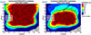 |
Figure 1 EGNOS APV-I combined daily availability for (a) pre-storm conditions on 3 November 2023, and (b) storm conditions on 4 November 2023 that corresponded to a significant decrease of the APV-I availability, especially in the Northern Europe (from >99.9% before the storm to ∼80% during the storm). This prompted the notification of “important/severe” degradation to be sent out, and represents one of only 25 occurrences since 2014 where such strong degradation occurred. |
2 Dataset
Over the past few decades, various observational techniques and instruments have been developed to study the Earth’s ionosphere and thermosphere, offering valuable opportunities to analyze the influence of geomagnetic storms on the IT system through coordinated observations on a global scale (Astafyeva et al., 2015; Nava et al., 2016; Zakharenkova et al., 2016; Aa et al., 2023a,b). In this Section, we describe the data sets used for analyzing the effects of 4–5 November 2023 geomagnetic storms on the ionosphere and thermosphere, to analyze the physical mechanisms behind the features highlighted as anomalous in the IsUG index maps.
2.1 UQRG VTEC maps
One of the most widely used ionospheric parameters is the total electron content, which represents the integrated electron density between the ground-based receivers and GNSS satellites (Garner et al., 2008). These measurements depend on the slanted path of the signal through the ionosphere and plasmasphere, and need to be converted into the vertical total electron content, which can be done, for instance, using mapping functions (Mannucci et al., 1998) or ionospheric tomography (Hernández-Pajares et al., 1999). Several well-established analysis centers are tasked with producing global ionospheric maps (GIMs) of VTEC for the International GNSS Service (IGS) (Hernández-Pajares et al., 2009). GIMs are typically provided in the IONosphere EXchange (IONEX) format with a spatial resolution of 2.5° × 5° geographic latitude (GLat) and longitude (GLon) and temporal resolution from 15 min to 2 h (the techniques used by different IGS analysis centers are described by Roma-Dollase et al., 2018). Within the IGS, the ionospheric working group (Iono-WG) is responsible for deriving the combined IGS GIMs by comparing results from different processing techniques and analysis centers within the community.
One of the VTEC GIMs with high temporal resolution (15 min) and accuracy is the UPC Quarter-hour resolution Rapid GIM (UQRG, Roma-Dollase et al., 2018). UQRG maps are generated by UPC-IonSAT on a daily basis and with a latency of less than 2 days (rapid in IGS terminology) and are available since end of 1996, for instance from the PITHIA e-Science Centre developed under the EU-funded project PITHIA-NRF. The UQRG VTEC GIMs, derived using a two-layer ionospheric tomography, are able to capture realistic features, including in complex regions corresponding to sparse data coverage, such as the polar ionosphere (Hernández-Pajares et al., 2020). They have been used in various applications, for instance, to mitigate efficiently the Faraday rotation induced by the ionosphere in the Low Frequency Array (LOFAR) radioastronomical measurements (Porayko et al., 2023), to generate GIMs of VTEC gradients, and GIMs of ionospheric storm scale indices, fully consistent with the ones generated from raw GNSS measurements with completely different techniques by other authors, as is respectively shown in Liu et al. (2021, 2022). UQRG maps have been proven to be amongst the most reliable GIMs (Adil et al., 2025) and are frequently used by the community (e.g. Nava et al., 2016; Yasyukevich et al., 2018; Zhang & Zhao, 2019; Babu Sree Harsha et al., 2020; Cesaroni et al., 2020; Krishna & Ratnam, 2020; Younas et al., 2020, 2022, 2023; Wielgosz et al., 2021; Wu et al., 2021; Zhukov et al., 2021; Adolfs et al., 2022; Campuzano et al., 2023; Long et al., 2024; Xi et al., 2024, among others).
2.2 Ionospheric storm-time index IsUG
Due to the fact that VTEC values can be vastly different depending on solar activity levels, seasons, local times, and geomagnetic disturbances, Liu et al. (2021) introduced a normalized storm scale index IsUG, which is derived as follows. Using the global UQRG VTEC maps, hourly mean values are derived for every cell on the 2.5° × 5° GLat-GLon grid. These values are subtracted from the 27-day means for the same cell and local time, thus removing the diurnal and seasonal variations, as follows:
 (1)
(1)
where GTEC represents the hourly averaged values, and RTEC is the 27-day averaged value. The 27-day period was chosen as it is consistent with the solar rotation period (for details, see Liu et al., 2021). The values are further normalized by their mean values (μ) and standard deviations (σ) from 1997 to 2014, calculated for every hour and season for each grid cell. The normalized IsUG index can be written down as follows:
 (2)
(2)
After analyzing the statistical distributions of IsUG, Liu et al. (2021) developed an empirical scale of values corresponding to the quiet, negative and positive storm effects, at moderate, strong or severe intensity levels (see Table 1), including the corresponding percentage of occurrence during 1997–2014. Using IsUG allows one to generate realistic global maps of the ionospheric disturbance levels that can be analyzed consistently and compared across varying seasons, local times and geographic locations. Liu et al. (2021) presented statistical analysis of the IsUG values, but the index has not been used for detailed case studies of ionospheric storms yet. Throughout this study, by ionospheric anomalies we specifically refer to variations of the IsUG index: positive IsUG values correspond to VTEC enhancements relative to the 27-day climatological baseline (normalized for solar-cycle and seasonal conditions), whereas negative IsUG values indicate relative VTEC depletions.
The definition and occurrence probability of IsUG derived from UQRG GIMs during the period 1997–2014 (reproduced from Liu et al. (2021)).
2.3 Thermospheric data from GOLD, TIMED and GRACE-FO missions
Thermospheric variability plays an important role in the ionospheric morphology during geomagnetic storms, and therefore we use several available data sets to compare features seen in VTEC and IsUG to the known physical mechanisms. To evaluate the high-latitude thermospheric heating, we use observations by the Global-scale Observations of the Limb and Disk (GOLD) mission. GOLD represents a spectrograph observing Earth’s ultraviolet (UV) emissions at wavelengths from 134 to 162 nm (Eastes et al., 2017; McClintock et al., 2020). The measurements are conducted using two channels (denoted as A and B) in a tilted orientation that allows scanning either the Northern or Southern hemisphere by using two back-to-back plane mirrors. GOLD is placed at the geostationary orbit (−47.5° longitude) and provides scans of a fixed geographic region from −120° to 20° GLon and completes a full-disk scan every ∼2 h from around 8:30 to about 18:30 UT. There are several observational modes, including the occultations, day disk scans and limb scans, that allow deriving several key parameters of the neutral thermosphere (Gan et al., 2024). The TDISK product, provided in the Level 2, contains the effective neutral atmospheric temperatures derived from day disk observations of N2 Lyman-Birge-Hopfield (LBH) emissions and can be used to evaluate the high-latitude heating during storms (for details, see Evans et al., 2024).
To evaluate changes of the thermospheric composition, we use O/N2 observations performed by the Global Ultraviolet Imager (GUVI) onboard the Thermosphere, Ionosphere, mesosphere Energetics and Dynamics (TIMED) satellite (Christensen et al., 2003). The TIMED mission has been operating since 2001, providing observations of several thermospheric quantities, focusing particularly on the lower thermosphere. The GUVI instrument takes spectroradiometric measurements of the far UV (FUV) airglow emission from 120 to 180 nm that are typically due to the major upper atmospheric species (H, O, N2 in emission and O2 in absorption) (Meier et al., 2015). The GUVI observations are used to derive the O/N2 column ratios below the satellite orbit of ∼625 km, providing a global picture every ∼15 orbits (e.g. Astafyeva et al., 2015).
To assess the thermospheric expansion during the 4–5 November events, we use the neutral density observations by the Gravity Recovery and Climate Experiment Follow-On (GRACE-FO) mission. GRACE-FO was launched in May 2018 and consists of two identical satellites on near-polar orbits with altitudes of ∼500 km (Flechtner et al., 2012). Both GRACE-FO satellites are equipped with high precision triaxial accelerometer instruments that allow measuring non-gravitational forces and provide information about the satellites’ linear and angular accelerations (Behzadpour et al., 2021; Siemes et al., 2023). In particular, Siemes et al. (2023) developed an improved method of modeling the radiation pressure (see also Hładczuk et al., 2024) and a consistent calibration technique, which allowed for a derivation of neutral densities along the satellite orbit from accelerometer observations. The corresponding data are provided in open access by the TU Delft.
2.4 LSTID catalog
Ionosondes provide ground-based measurements of relevant ionospheric observables that can be useful to characterize the geomagnetic storm effects. In particular, they play a crucial role in monitoring LSTIDs by providing real-time measurements of ionospheric characteristics such as Maximum Usable Frequency at 3000 km (MUF(3000)) and critical frequency of the F2 layer (foF2). The high-frequency interferometry (HF-INT) method, developed by Altadill et al. (2020), processes data from a comprehensive network of European ionosondes through the Global Ionospheric Radio Observatory (GIRO) DIDBase Fast Chars database in near-real time, identifies quasi-periodic oscillations in the MUF(3000) across multiple ionosonde locations and, performing spectral analysis, detects and characterizes LSTID events by calculating the amplitude, the dominant oscillation period, and the propagation velocity vector. A more detailed explanation of the HF-INT method can be found in Altadill et al. (2020). Based on the results from this method, a detailed LSTID event catalog has been compiled, documenting observed LSTID events with parameters such as onset time, duration, and the average dominant period, amplitude, and propagation velocity for the event duration. This comprehensive open-access catalog is detailed in Segarra et al. (2024) and provides an organized and systematic record of LSTID events over Europe from 2014 to 2023.
3 Results
In this Section, we present observational results for the 4–5 November 2023 events. We first analyze the solar and geomagnetic conditions during this time period, and then show a detailed examination of how these fluctuations influenced the VTEC, analyze the storm-time features highlighted in IsUG maps and the corresponding chain of processes in the ionosphere-thermosphere system.
3.1 Solar wind and geomagnetic conditions
The period of the study corresponded to complex heliospheric conditions. Below, we give an overview of solar and geomagnetic conditions during these events, while the in-depth analysis from L1 in-situ data was presented by Gil et al. (2024), accompanied with modeling results of the EUropean Heliospheric FORecasting Information (EUHFORIA) code (Poedts et al., 2020) . According to their results, the moderate geomagnetic activity on 4 November appears consistent with a corotating interaction region (CIR) reaching Earth. Solar wind density started increasing around 12:45, while the velocity remained low (around ∼330 km/s, which is below the usual quiet-time levels). It should be noted that this event exhibited a sudden storm commencement in the SYM-H index (Fig. 2), which is not typical for CIR-driven storms (Borovsky & Denton, 2006). This was most likely caused by the pressure step due to increased solar wind density. However, the EUHFORIA simulations reveal a glancing hit by a CME, which was propagating southward from the Earth and likely contributed to the SSC formation. IMF Bz reached −13 nT during the storm main phase. The corresponding SYM-H values reached about -60 nT, and maximum Kp level was 4.67. The main phase of the event lasted up until around ∼23:00 (Fig. 2g). Around midnight, the IMF turned northward, and the recovery phase began, lasting for approximately 12 hours. In general, the 4 November event was moderate and relatively short-lived, as SYM-H recovered to almost the pre-storm levels already ∼12 h after the main phase, and Kp levels returned down to 2.0.
 |
Figure 2 Solar wind and geomagnetic conditions during the period of this study. The times of three sudden storm commencements are marked with yellow vertical lines. |
On 5 November, two CMEs hit Earth, producing a strong double-dip geomagnetic storm, classified as a G3 event by NOAA. Gil et al. (2024) note that according to EUHFORIA simulations, these CMEs were propagating through the ongoing CIR. Sheath encounters on 5 November could be identified by increases in the solar wind velocity, density, and plasma β (Fig. 2). Inside the magnetic flux ropes, most of these parameters dropped relative to the sheath, while magnetic field showed smooth rotation, consistent with typical CME signatures (Gil et al., 2024). The rapid southward turning of the IMF around 09:00 UT (reaching −19 nT) and a spike in the solar wind dynamic pressure led to an SSC as seen in the SYM-H index around 09:30 UT. This period also corresponded to a sharp increase of the Kp index (from 2 to 5.67). The second SSC occurred later in the day around 14:00 due to the arrival of the next sheath. IMF Bz magnitude reached −21 nT and remained negative for a prolonged time, leading to a strong minimum of SYM-H of −188 nT and maximum Kp value of 7.33. The main phase of this even lasted until ∼17:00, and the recovery phase lasted for approximately 2 days and corresponded to relatively low IMF magnitudes. EUHFORIA simulations of Gil et al. (2024) indicate the first CME encounter to be glancing, while the second impact was more central; both of them interacted with an ongoing CIR, thus producing a non-textbook storm morphology.
Due to close activation times of the 4 and 5 November events (the recovery after the 4 November event lasted ∼12 hours) and mixed driving, we avoid describing them as independent storms. Instead, when analyzing the ionosphere-thermosphere changes, we view them as parts of the same composite storm. To avoid confusion with the conventional storm-phase terminology (main and recovery phases that refer to periods of ring current buildup and return to quiet conditions, respectively), we refer to the 4 and 5 November activity periods as events rather than phases throughout the paper.
3.2 VTEC and IsUG variations
Figure 3 shows global UQRG maps of the total electron content during the moderate event on 4 November 2023, including the recovery phase the following day. In the pre-storm phase, shown in the top row of Figure 3, the global VTEC morphology followed the expected quiet-time behavior. A hemispheric difference could be seen in VTEC, with higher values in the Southern hemisphere. This period falls within the December solstice (D) season, based on the classification by Lloyd (1874), which divides the year into three four-month intervals: D-season (November–February) and J-season (May–August), centered on the solstices, and E-season (March–April and September–October) combining months around the two equinoxes. As November is at the beginning of the D-season, it generally corresponds to local summer conditions in the Southern Hemisphere and higher ionization rates. In general, a pronounced EIA could be seen before the storm, with the Northern crest being stronger than the Southern one (e.g. at 14 UT). The VTEC values were elevated during the storm compared to the pre-storm conditions around the EIA crests. During the main phase of the event, one could see a development of the storm-enhanced density (SED) plume in the North American region starting around 20:00 UT and persisting for approximately 4 hours. The VTEC values in the SED plume were approximately 50% higher compared to the conditions on 3 November, which are considered to be quiet times (Fig. S1.1 in the Supplementary Material S1). During the main phase, pronounced VTEC enhancements by up to ∼100% could be seen around the auroral oval (Figs. 3 and S1.1). In the Northern hemisphere, they persisted from 18 UT on 4 November until ∼02 UT on 5 November, while in the Southern hemisphere they could be seen until 08 UT on 5 November.
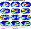 |
Figure 3 VTEC evolution during the 4 November event. VTEC was mostly enhanced, both at high latitudes and around the EIA crests. In the main phase, a SED plume developed over the North American sector around 22:00 UT. |
Figure 4 shows maps of the IsUG storm-time index during the 4 November event (the level specification for this index is given in Table 1). During the pre-storm conditions, the IsUG values remained generally within the quiet range (within ±1), showing only minor variations (top row of Fig. 4). During the main phase, one could observe intense enhancements of IsUG at high latitudes, with positive values ∼4–5, which indicate strong-to-severe positive enhancements of VTEC compared to the 27-day averages. While the initial high-latitude increases were observed already around 20:00 UT on 04 November 2023, the enhancements around the EIA crests first manifested 1–2 hours later, around 21–22 UT. These enhancements also correspond to positive ionospheric storm phases, and indicate strengthening of the equatorial plasma fountain effect. In comparison with raw VTEC values shown in Figure 3, one can see that the EIA crests extended to slightly higher latitudes compared to the pre-storm conditions. Based on the storm-time TEC index, the 4 November event was mostly positive, with no strong negative phase. While some negative disturbances could be observed during the recovery phase in the Southern hemisphere, they were mild and rather localized compared to strong global enhancements of VTEC seen during the main phase.
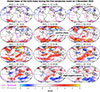 |
Figure 4 Ionospheric storm-time index IsUG during the 4 November 2023 event. The pre-storm values remained close to zero, while during the storm one could see the development of a strong positive phase at high and mid-latitudes, followed by a weak negative phase ∼8 hours later, localized in the Southern hemisphere. |
VTEC variations during the strong event on 5 November (Fig. 5) were markedly different from those during the preceding moderate activity period. During the main phase of the storm, one could see a strong intensification of the equatorial ionization anomaly crests (around 15–20 UT on 05 November), as well as extension of the EIA up to ∼40°–50° quasi-dipole latitude (QDLat), indicating the formation of the superfountain effect (second row in Fig. 5). In the Northern hemisphere, an SED plume could be seen over the North American region during the main phase, starting from ∼18 UT until ∼22 UT. The superfountain effect was particularly strong in the American sector, as shown in the VTEC keograms presented in the Supplementary Material S1 (Fig. S1.2). The corresponding VTEC values were up to 100% higher compared to the quiet times (Fig. S1.1 in the Supplementary Material S1). In terms of the ionospheric storm-time index, these initial TEC enhancements during the 5 November event were classified as severe positive effects (Fig. 6).
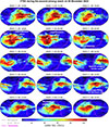 |
Figure 5 VTEC evolution during the strong storm on 5 November 2023. In the main phase (around 18–20 UT), a strengthening of the EIA could be observed, as well as a formation of a SED plume around North America. However, already by 22:00 UT the EIA crests weakened, and subsequently a strong negative phase has developed. |
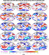 |
Figure 6 IsUG variations during the strong storm on 5 November 2023. In the main phase, there were strongly positive high-latitude VTEC enhancements that quickly involved low and equatorial latitudes. Around 22:00 UT on 05 November, a negative storm phase started to develop. Over the following day, an extreme negative phase occurred, with most pronounced effects in the Southern hemisphere. |
During the 5 November event one could see the formation of an intense negative phase during the storm’s recovery starting from around 22 UT, manifested as weakening and merging of the EIA crests and appearance of dark blue regions at mid-latitudes in Figure 5. The normalized storm-time ionospheric index reveals severe negative changes occurring at mid- and high latitudes (Fig. 6). The depletions of VTEC in the corresponding regions lasted for over 36 hours, until around 12–16 UT on 7 November (see also Figs. S1.3 and S1.4 in the Supplementary Material S1). There was a pronounced hemispheric difference in VTEC during the negative phase, with more intense negative effects in the Southern hemisphere. Furthermore, strong longitudinal differences could be observed in the Southern hemisphere, with much stronger negative effects around Indian and Southern oceans compared to other longitudinal sectors. In the Discussion Section, we offer the interpretation of these asymmetries in relation to thermospheric variations, which are presented in the following Subsection.
3.3 Thermospheric observations by GOLD, TIMED and GRACE-FO missions
Ionospheric variations during geomagnetic storms are strongly influenced by changes in the global circulation of the Earth’s thermosphere (Fuller-Rowell et al., 1994, 1996; Rishbeth, 1998), and in order to show that differences between the later stages of the two events highlighted by IsUG are reflective of realistic physical processes, in this subsection we present observations of the neutral temperatures, densities and composition to later discuss them in combination with the ionospheric changes presented above.
Figure 7 shows O/N2 observations by the GUVI instrument onboard TIMED. During the quiet day on 3 November, there was a strong hemispheric asymmetry, with O/N2 values in the Northern hemisphere in the order of 1.4 compared to ∼0.5 in the Southern hemisphere. During storm-times, the O/N2 distributions were significantly modified. While the values remained relatively stable on 4 November, on 5 November the hemispheric asymmetry was exacerbated and a pronounced depletion down to ∼0.2 appeared around the Southern ocean. It further intensified during the recovery phase of the storm, with values ∼3–4 times lower than during quiet conditions. These regions corresponded to the strongest depletions of VTEC (Figs. 5–6). During the recovery phase after the 5 November event, the O/N2 ratios in the Southern hemisphere showed signs of replenishment around 7–8 November but did not return to their pre-storm values.
 |
Figure 7 O/N2 observations by TIMED/GUVI. A strong decrease occurred in the Southern hemisphere during the 5 November event, with values dropping by a factor of 4 compared to quiet times. |
Figure 8 shows the neutral temperature scans observed by GOLD. Each of the presented images accumulates two scans to provide a global view of both hemispheres. The neutral temperatures did not exhibit significant enhancements during the beginning of the main phase of the 4 November event (scan at 18:30 UT) compared to the quiet-time conditions on 3 November. During the strong event on 5 November, however, there was a notable intensification of neutral temperatures by ∼300 K at high latitudes around the main phase (18:30 UT scan in Fig. 8). The GOLD scans reveal much stronger high-latitude heating compared to quiet times and the 4 November event, as well as an additional equatorial temperature increase. It should be noted that while the scan on 5 November was obtained during the peak of the main phase, for the 4 November event, the scan at 18:30 corresponded to the beginning of the main phase and may not be representative of all the high-latitude heating during the event. For this reason, we complement the GOLD temperature scans with observations of the neutral thermospheric densities by GRACE-FO, shown in Figure 9, that can also be used to evaluate the thermospheric expansion. During the period of the study, GRACE-FO crossed the equator at dawn and dusk sectors (around 06 and 18 hours of magnetic local time). During the two activity periods investigated in this study, one could observe high-latitude neutral density enhancements around the times of spikes in the merging electric field (for the calculation details, see Zhou et al. (2016) and the Hp30 index (Yamazaki et al., 2022). These enhancements subsequently propagated towards the equator, on timescales of around 5–6 hours. During the 4 November event, neutral densities were enhanced by a factor of ∼1.5 compared to quiet times, and the equatorward propagation could be observed in both MLT sectors covered by GRACE. The density enhancements were stronger in the Southern hemisphere and propagated into the Northern hemisphere above the equator (00-06 UT on 5 November). During the period of stronger activity on 5 November, the density also propagated equatorwards from high latitudes. Neutral densities increased by a factor ∼5 compared to the pre-storm conditions, which is much higher than during a milder 4 November event.
 |
Figure 8 Neutral thermospheric temperature scans by GOLD. Neutral temperatures showed pronounced increases around the main phase of the storm at high latitudes (around 18:30 UT on 5 November). |
 |
Figure 9 (a) Geomagnetic Hp30 index, (b) merging electric field, and neutral density observations by GRACE-FO (c) in the dawn and (d) dusk sectors (local times of equatorial crossings 7.5 and 19.5 hours, respectively) throughout the period of the study. |
3.4 LSTIDs
Segarra et al. (2024) catalog reports two distinct LSTID events associated with the 4–5 November geomagnetic storm (see Table 2). Additionally, the catalog reports an extra event in the morning of 4 November, which is related to the solar terminator and thus not attributable to storm activity. Note that the parameters shown in Table 2 correspond to the averages for all the active ionosonde sites for the duration of the LSTID event. During the 4 November event, LSTIDs in Europe began around 19:20 and lasted for 4.1 hours. As reported in the catalog, these LSTIDs propagated southwest with a velocity of 642.62 m/s (with a standard deviation of 76 m/s across all stations shown in Fig. 10). The second LSTID event, recorded on 5 November at 16:15 UT corresponded to the peak of the main phase. During this event, LSTIDs had longer duration of ∼7.3 hours compared to 4.1 hours on 4 November; they also had higher velocities of >∼750 m/s (±96 m/s) that were roughly consistent across all ionosondes (Fig. 10b), except for unusually high velocities (1268 ± 214 m/s) at Juliusruh. The LSTIDs were propagating southward, indicating strong equatorward disturbance neutral winds acting during the 5 November event, compared to less intense winds propagating southwest on 4 November. Figure 10 presents the snapshots of the HF-INT method for the main phases of the 4 and 5 November events, while the full evolution of the velocity vectors is provided in the Supplementary (animations S2 and S3). It should be noted that we use data from the European ionosonde network, as they are available through the Segarra et al. (2024) catalog, and this does not imply the absence of LSTIDs in other longitudinal sectors, where a similar analysis can be performed in future studies.
LSTID events during the 4–6 November 2023 geomagnetic storm from the Segarra et al. (2024) catalog.
 |
Figure 10 Snapshots indicating LSTID activity over Europe on 4 November (a) and 5 November (b) obtained from ionosonde data using the HF-INT method. During the 5 November storm, the LSTID velocities were around 750 m/s and propagated towards the equator, while during the 4 November event the velocities were lower and their vectors were directed southwest. |
4 Discussion
Ionospheric storms are characterized by complex patterns that relate to a multitude of drivers, including electrodynamics, changes of the neutral atmospheric composition and circulation patterns, among others (Mendillo, 2006; Prölss, 2008; Prölss, 2011). The interplay of these drivers is unique for every storm, as shown by many studies analyzing individual events (Astafyeva et al., 2015; Nava et al., 2016; Zakharenkova et al., 2016; Zhou et al., 2016; Cherniak & Zakharenkova, 2017; Aa et al., 2023a,b; Aa et al., 2024b). Even though a significant progress in ionospheric monitoring has been made over the past few decades, developing an ionospheric index that would reflect realistic anomalies on the global scale has been challenging and represents an active area of research. In this study, we use the recently developed IsUG index for a case study of 4–5 November 2023 events and assess its ability to track ionospheric disturbances resulting from physical processes in the IT system.
The moderate geomagnetic activity on 4 November started at around 18:00 UT, with the southward turning of IMF Bz that reached the value of −13 nT and increase in the merging electric field to around 4 mV/m. Around the same time, IsUG maps showed strong positive anomalies at high latitudes, which corresponded well with VTEC enhancements around the auroral oval (Figs. 3 and 4). These enhancements quickly intensified, and around ∼2 hours later positive anomalies could be observed around the EIA crests (Figs. 3 and 4). We interpret these positive changes as the consequence of PPEF acting within the first few hours of the storm. PPEFs generally result from the fast equatorward expansion of the high-latitude convection patterns (Tsurutani et al., 2007). They are known to enhance the eastward component of the equatorial electric field on the dayside, leading to stronger upward E × B drift (Scherliess & Fejer, 1997; Fejer & Scherliess, 1997; Xiong et al., 2016). The enhanced upward drifts lift electrons to higher altitudes which correspond to lower recombination rates, allowing these electrons to remain there for longer times. When transported downward due to ambipolar diffusion, they enhance the EIA (Mendillo, 2006; Zhou et al., 2016). While PPEF effects during daytime lead to positive ionospheric effects, they produce negative VTEC changes on the nightside. Namely, they enhance the westward component of the equatorial electric field leading to the downward E × B drift pushing the electrons into lower layers of the atmosphere with higher recombination rates. During the 4 November event, slight negative anomalies in IsUG could be seen on the nightside around 18–20 UT (Fig. 4), consistent with the PPEF action.
The negative phase following the 4 November event was moderate and rather localized. Approximately 10 hours after the storm commencement, negative IsUG values (corresponding to decreases of VTEC) could be seen in the Southern hemisphere, particularly in the region of Indian and Southern oceans (Fig. 4). They coincide with the depletions of O/N2 ratios seen by TIMED/GUVI (Fig. 7). The O/N2 depletions indicate the uplift of the molecular-rich fraction of the neutral gas from low to high altitudes leading to increased recombination rates, and their link to the formation of the negative storm phases is now well established (Prölss, 2008; Prölss, 2011; Astafyeva et al., 2015; Grandin et al., 2015). The O/N2 values in the Southern hemisphere decreased from the quiet-time value of ∼0.4 to about 0.2 during the event around the region of VTEC depletions (Figs. 7 and 4), and therefore, the observed negative changes are most likely attributed to the thermosphere composition changes. On the other hand, in the Northern hemisphere there were increases in O/N2 ratios and the VTEC changes remained largely positive for the entire duration of the storm (Fig. 4). It should be noted that the maximum latitude sampled by TIMED during the event was around 45° and therefore the coverage of GUVI data does not allow analyzing the Northern hemisphere in sufficient detail, while O/N2 scans by GOLD, shown in the Supplementary Material S1 (Fig. S1.5), provide a broader latitudinal coverage and allow analyzing hemispheric differences. A strong hemispheric asymmetry can be observed in GOLD O/N2 data, with an increase in the Northern hemisphere compared to quiet times (e.g. around 10:30 on 5 November in Fig. S1.5). Due to the fact that the ion production rate generally depends on the concentration of atomic oxygen (Fuller-Rowell et al., 1996), the positive VTEC effects in the Northern hemisphere can be attributed to the increase in the atomic oxygen fraction.
During the much stronger 5 November storm, the positive effects tracked by IsUG were generally similar to the first event, with changes initially occurring at high latitudes and quickly involving the mid- and low latitudes. However, unlike during the 4 November event, there was a notable superfountain effect developing in the first few hours of the storm on 18–20 UT (highlighted with white arrows in Fig. 5). The superfountain-related EIA changes, which involved the extension of the crests up to 40–5° QDLat with increases of VTEC by up to 100%, were classified as severe positive effects in IsUG (Fig. 6; see also Fig. S1.1). We attribute development of the superfountain effect within the first 4 hours of the main phase to a strong PPEF action. As discussed by Tsurutani et al. (2007), during large storms, the strong southward IMF leads to much stronger magnetospheric convection. It creates intense dawn-to-dusk electric field that is superimposed onto the quiet-time eastward equatorial electric field on the dayside, leading to much stronger upward E × B drift lifting the plasma to higher altitudes, sometimes up to 900 km (Lu et al., 2013). Due to the subsequent ambipolar diffusion along the field lines, these particles end up at higher latitudes compared to the quiet times. Figure S1.6 in the Supplementary Material S1 shows the equivalent convection patterns for the period of the study, obtained from the ground-based magnetometer observations by the SuperMag network (Gjerloev, 2012). The convection pattern was much stronger during the 5 November event, which agrees well with the formation of the superfountain effects. An additional way to detect the PPEF action, frequently used in ionospheric studies, is by examining ground magnetic field observations, usually in terms of the difference between one equatorial station and one magnetometer located a few degrees off the magnetic equator (Anderson et al., 2002). For the period of 4–5 November, the magnetometer data were analyzed extensively by Agyei-Yeboah et al. (2025) and also confirm the presence of PPEFs during the initial phases of both events.
The positive phase of the 5 November event was relatively short-lived, and already 3–4 hours after the storm commencement the negative phase started to develop (Figs. 5–6). The negative changes in TEC continued to develop over the following 18 hours and could still be observed for up to 36 hours after the storm commencement (see Figs. S1.3–S1.4 in the Supplementary Material S1). We interpret these negative changes as the consequence of the strong expansion of the neutral atmosphere and resulting thermospheric changes. In particular, the strong high-latitude input led to a strong enhancement of the thermospheric neutral temperature around the main phase (∼18–19 UT on 5 November), seen in GOLD scans (Fig. 8), where temperatures at high latitudes exceeded 1200 K compared to around ∼870 K during the quiet times two days prior. Additionally, thermospheric neutral densities at high latitudes, obtained from accelerometer observations on GRACE-FO, have also seen a significant increase by approximately a factor of 5 compared to quiet times, which also contributed to changing the pressure balance of the neutral thermosphere. The consequences of this intense heating (by over 300 K) and neutral density increase are two-fold. Firstly, strong gradients with respect to the equator are known to drive strong equatorward winds, which set up disturbance dynamo currents that affect the equatorial electrodynamics (Blanc & Richmond, 1980; Richmond et al., 2003). The action of disturbance winds could indeed be seen during the 5 November event starting approximately 4 hours after the storm commencement, manifested by a pronounced weakening of the EIA (Fig. 5 at 22:00). DDEFs take around 4 hours to develop and invert the equatorial electric field to the westward direction, and therefore the EIA weakening is in line with the DDEF development.
The second major consequence of the high-latitude storm-time heating is the uplift of the molecular-rich fraction of the neutral air to higher altitudes, which decreases O/N2 ratios in the respective regions. This effect could indeed be seen in TIMED observations in Figure 7. In the East-Antarctic region, where the most pronounced negative TEC effects occurred, the corresponding O/N2 ratios were particularly low, dropping by approximately a factor of 3–4 compared to the quiet times (Fig. 7). The resulting increases in recombination rates provide the most likely explanation of the respective severe negative anomalies in IsUG. The strong hemispheric asymmetry in O/N2 observed during the event, with stronger drops in the Southern (local summer) hemisphere, can be explained by higher efficiency of the thermospheric expansion during the local summer conditions. In particular, the conductivity due to solar production is higher in the local summer hemispheres, which adds to the Joule heating source by >50% compared to the local winter conditions (Fuller-Rowell et al., 1996). Therefore, the expansion of the molecular-rich air during storm times is expected to occur more efficiently in the local summer hemisphere (in our case, the Southern hemisphere). The corresponding depletions O/N2 in ratios to extremely low values agree well with this explanation. Additionally, the storm-time disturbance neutral winds in the local summer hemispheres are aligned with the background thermospheric summer-to-winter circulation. Therefore, during storms these winds are enhanced and help transport the composition changes to mid- and low latitudes (Fuller-Rowell et al., 1994, 1996). This effect could be seen during the 5 November event, with depletions of O/N2 ratios extending down to the equatorial latitudes (Fig. 7) causing additional depletions of VTEC.
It should also be noted that the 4 November event corresponded to a relatively mild CIR-driven storm, although a potential glancing CME encounter has been identified by Gil et al. (2024). It had a very low solar wind velocity below the average quiet-time levels (around 330 km/s). Nevertheless, this event corresponded to strong southward IMF Bz (−13 nT) and produced changes in the ionosphere that were classified as severe by the EGNOS system, limiting the APV-I availability over Europe. This event underscores the role of solar wind density and IMF Bz polarity on the ionospheric morphology, and gives useful hints for improving the existing empirical models of the ionosphere. Our results demonstrate that the history of several solar wind parameters, including IMF Bz and solar wind velocity and pressure, might need to be considered as driving parameters for the empirical models, alongside the traditional inputs such as Kp and F10.7.
5 Summary and conclusions
Finding ionospheric indices that are suitable for real-time monitoring and represent realistic structures has traditionally been a challenge due to the highly non-linear nature of ionospheric dynamics, driven by both the internal variability and coupling with the magnetosphere and thermosphere. In this study, we analyze the morphology of the ionosphere-thermosphere system on 4–5 November 2023, and evaluate the ability of the recently developed IsUG index maps to track the ionospheric anomalies in relation to the underlying physical processes. The complex heliospheric conditions during this period caused a composite geomagnetic storm with two activity periods: a moderate disturbance on 4 November caused by a CIR compression, and an intense event on 5 November following the additional arrival of two successive CMEs. In both cases, IsUG highlighted initial positive anomalies, which we attribute to prompt penetration electric field (PPEF) effects during the first few hours of both events. On 5 November, stronger convection led to the development of a superfountain effect in the American sector, marked as a severe positive anomaly in IsUG. The delayed ionospheric responses of the two events were significantly different, with a weak and localized negative phase following the 4 November event and severe negative disturbances after the 5 November storm. This difference is linked to varying high-latitude heating. While during the first event the high-latitude heating was weak, an intense heating and thermospheric expansion could be seen during the 5 November storm, causing intense depletions of O/N2 ratios in the Southern hemisphere and disturbance neutral winds that redistributed these changes to low latitudes and caused global negative ionospheric effects.
Our results provide a case study highlighting the variability of the ionosphere-thermosphere system during complex geomagnetic storms. Analyzing such events and delineating the respective drivers is crucial for mitigating the hazards that they pose. Real-time monitoring of such events can be done, for instance, by using the ionospheric IsUG index that is derived from the UQRG VTEC maps. This paper is the first one to apply the IsUG to analyze processes during a geomagnetic storm as a case study. Our results show that features highlighted as anomalous by IsUG align well with physical processes in the ionosphere-thermosphere system depicted by other instruments. The IsUG index can be further updated in the future to take into account the events from the ongoing solar cycle 25 and can be used in various applications related to ionospheric research and space weather monitoring.
Acknowledgments
We thank the participating institutions of the PITHIA-NRF European project for establishing the collaborative infrastructure that enabled access to data used in this study. The editor thanks two anonymous reviewers for their assistance in evaluating this paper.
Funding
This research has been supported by the European Union projects PITHIA-NRF (H2020-INFRAIA-2018-2020101007599) and DISPEC (HORIZON-565 CL4-2023-SPACE-01-71). A.S. is funded by Deutsche Forschungsgemeinschaft (DFG), project number 520916080. E.K. is supported by the DFG Heisenberg grant under number 516641019.
Conflicts of interest
The authors declare no conflicts of interest.
Data availability statement
The solar (wind) data and the SYM-H index were obtained from the OMNIWeb database (https://omniweb.gsfc.nasa.gov/). The Hp30 and Kp indices are provided by GFZ Potsdam (https://kp.gfz-potsdam.de/hp30-hp60). GRACE-FO densities were obtained from TU Delft through the FTP server ftp://thermosphere.tudelft.nl. The GOLD Level 2 data are available at the GOLD Science Data Center and at NASA’s Space Physics Data Facility https://spdf.gsfc.nasa.gov/pub/data/gold/level2/. UQRG maps are available through the e-center of PITHIA-NRF European Union project (https://esc.pithia.eu/data-collections/DataCollection_UPC-RapidNetwork_GIM/).
Supplementary material
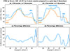 |
Fig. S1.1: Latitudinal profiles of VTEC in the American sector (GLon = -100°) for the 4 and 5 November events compared to the quiet-time baseline on 3 November. All the curves are for 20:00 UT. During the 4 November event, VTEC was enhanced mainly at high latitudes, by up to 50-100%, and also formed an SED plume where VTEC was enhanced by ~70%. During the 5 November storm, a notable superfountain effect could be seen, with the EIA crests extending up to ~30-40° QDLat (see also Figure 5 in the main text), and the corresponding VTEC increases by up to 100%. |
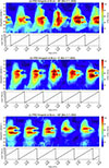 |
Fig. S1.2: UQRG VTEC keograms for the American (a), European (b) and Australian (c) sectors during the period of the study. In the American sector, a notable superfountain effect was formed around 18-20 UT on 5 November (during the storm’s main phase consistent with PPEF action). In the Australian sector, one could observe merging of the EIA crests in the recovery phase of the storm, consistent with thermospheric changes (strongly depleted O/N2 ratios in the region). |
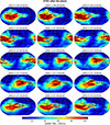 |
Fig. S1.3: VTEC maps on 6-7 November 2023 (after the storm). |
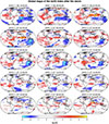 |
Fig. S1.4: Global maps of the IsUG index on 6-7 November 2023 (after the storm). The negative phase could be seen up to 10 UT on 7 November. |
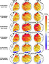 |
Fig. S1.5: GOLD O/N2 scans for the period of the study. During the main storm on 5 November 2023, O/N2 ratios were enhanced at mid-latitudes in the Northern hemisphere but showed a strong decrease at high-latitude regions in the Southern hemisphere. |
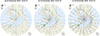 |
Fig. S1.6: Equivalent convection patterns derived from Supermag. During the first moderate event on 4 November, one could see enhanced convection compared to the quiet conditions on 3 November. During the strong 5 November event, the convection patterns were much stronger and expanded down to 40° of latitude. |
Supplementary animation S2: Access Supplementary Material
Supplementary animation S3: Access Supplementary Material
References
- Aa, E, Dzwill P, Zhang SR, Erickson PJ. 2024a. A statistical analysis of the morphology of storm-enhanced density plumes over the North American sector. J Geophys Res Space Physics 129(6): e2024JA032750. https://doi.org/10.1029/2024JA032750. [Google Scholar]
- Aa, E, Zhang SR, Erickson PJ, Wang W, Qian L, et al. 2023a. Significant mid-and low-latitude ionospheric disturbances characterized by dynamic EIA, EPBs, and SED variations during the 13–14 March 2022 geomagnetic storm. J Geophys Res Space Physics 128(8): e2023JA031375. https://doi.org/10.1029/2023JA031375. [Google Scholar]
- Aa, E., Zhang SR, Lei J, Huang F, Erickson PJ, et al. 2024b. Significant midlatitude plasma density peaks and dual-hemisphere SED during the 10–11 May 2024 super geomagnetic storm. J Geophys Res Space Physics 129(11): e2024JA033360. https://doi.org/10.1029/2024JA033360. [Google Scholar]
- Aa, E, Zhang SR, Wang W, Erickson PJ, Coster AJ. 2023b. Multiple longitude sector storm-enhanced density (SED) and long-lasting subauroral polarization stream (SAPS) during the 26–28 February 2023 geomagnetic storm. J Geophys Res Space Physics 128(9): e2023JA031815. https://doi.org/10.1029/2023JA031815. [Google Scholar]
- Adil, MA, Hadas T, Yang H, Hernandez-Pajares M. 2025. Quality assessment of the real-time global ionospheric maps following varying solar dynamics and a severe geomagnetic storm. GPS Solut 29(1): 1–16. https://doi.org/10.1007/s10291-024-01811-7. [Google Scholar]
- Adolfs, M, Hoque MM, Shprits YY. 2022. Storm-time relative total electron content modelling using machine learning techniques. Remote Sens 14(23): 6155. https://doi.org/10.3390/rs14236155. [Google Scholar]
- Agyei-Yeboah, E, Fagundes PR, Tardelli A, Pillat VG, Vieira F, et al. 2025. Global ionospheric response to a G2 and a G3 geomagnetic storms of November 4 and 5 2023. Adv Space Res https://doi.org/10.1016/j.asr.2025.01.046. [Google Scholar]
- Altadill, D, Segarra A, Blanch E, Juan JM, Paznukhov VV, et al. 2020. A method for real-time identification and tracking of traveling ionospheric disturbances using ionosonde data: first results. J Space Weather Space Clim 10: 2. https://doi.org/10.1051/swsc/2019042. [CrossRef] [EDP Sciences] [Google Scholar]
- Anderson, D, Anghel A, Yumoto K, Ishitsuka M, Kudeki E. 2002. Estimating daytime vertical ExB drift velocities in the equatorial F-region using ground-based magnetometer observations. Geophys Res Lett 29(12): 37–31. https://doi.org/10.1029/2001GL014562. [Google Scholar]
- Appleton, E, Ingram L. 1935. Magnetic storms and upper-atmospheric ionisation. Nature 136(3440): 548–549. https://doi.org/10.1038/136548b0. [Google Scholar]
- Astafyeva, E, Zakharenkova I, Förster M. 2015. Ionospheric response to the 2015 St. Patrick’s Day storm: a global multi-instrumental overview. J Geophys Res Space Physics 120(10): 9023–9037. https://doi.org/10.1002/2015JA021629. [Google Scholar]
- Babu Sree Harsha P, Venkata Ratnam D, Lavanya Nagasri M, Sridhar M, Padma Raju K. 2020. Kriging-based ionospheric TEC, ROTI and amplitude scintillation index (S4) maps for India. IET Radar Sonar Navig 14(11): 1827–1836. https://doi.org/10.1049/iet-rsn.2020.0202. [Google Scholar]
- Behzadpour, S, Mayer-Gürr T, Krauss S. 2021. GRACE follow-on accelerometer data recovery. J Geophys Res Solid Earth 126(5): e2020JB021297. https://doi.org/10.1029/2020JB021297. [Google Scholar]
- Berkner, L, Wells H, Seaton S. 1939. Ionospheric effects associated with magnetic disturbances. Terr Magn Atm Electr 44(3): 283–311. https://doi.org/10.1029/TE044i003p00283. [Google Scholar]
- Blanc, M, Richmond A. 1980. The ionospheric disturbance dynamo. J Geophys Res Space Physics 85(A4): 1669–1686. https://doi.org/10.1029/JA085iA04p01669. [Google Scholar]
- Borovsky, JE, Denton MH. 2006. Differences between CME-driven storms and CIR-driven storms. J Geophys Res Space Physics 111(A7): A07S08. https://doi.org/10.1029/2005JA011447. [Google Scholar]
- Bowman, G. 1965. Travelling disturbances associated with ionospheric storms. J Atm Terrestrial Phys 27(11–12): 1247–1261. https://doi.org/10.1016/0021-9169(65)90085-1. [Google Scholar]
- Bremer, J, Cander LR, Mielich J, Stamper R. 2006. Derivation and test of ionospheric activity indices from real-time ionosonde observations in the European region. J Atm Solar-Terrestrial Phys 68(18): 2075–2090. https://doi.org/10.1016/j.jastp.2006.07.003. [Google Scholar]
- Buonsanto, MJ. 1999. Ionospheric storms – a review. Space Sci Rev 88(3): 563–601. https://doi.org/10.1023/A:1005107532631. [CrossRef] [Google Scholar]
- Campuzano, SA, Delgado-Gómez F, Migoya-Orué Y, Rodríguez-Caderot G, Herraiz-Sarachaga M, et al. 2023. Study of ionosphere irregularities over the Iberian Peninsula during two moderate geomagnetic storms using GNSS and Ionosonde Observations. Atmosphere 14(2): 233. https://doi.org/10.3390/atmos14020233. [CrossRef] [Google Scholar]
- Cesaroni, C, Spogli L, Aragon-Angel A, Fiocca M, Dear V, et al. 2020. Neural network based model for global total electron content forecasting. J Space Weather Space Clim 10: 11. https://doi.org/10.1051/swsc/2020013. [CrossRef] [EDP Sciences] [Google Scholar]
- Cherniak, I, Zakharenkova I. 2017. New advantages of the combined GPS and GLONASS observations for high-latitude ionospheric irregularities monitoring: case study of June 2015 geomagnetic storm. Earth Planets Space 69: 1–14. https://doi.org/10.1186/s40623-017-0652-0. [NASA ADS] [CrossRef] [Google Scholar]
- Christensen, A, Paxton L, Avery S, Craven J, Crowley G, et al. 2003. Initial observations with the Global Ultraviolet Imager (GUVI) in the NASA TIMED satellite mission. J Geophys Res Space Physics 108(A12). https://doi.org/10.1029/2003JA009918. [Google Scholar]
- Eastes, R, McClintock WE, Burns A, Anderson D, Andersson L, et al. 2017. The global-scale observations of the limb and disk (GOLD) mission. Space Sci Rev 212, 383–408. https://doi.org/10.1007/s11214-017-0392-2. [CrossRef] [Google Scholar]
- Evans, JS, Correira J, Lumpe JD, Eastes R, Gan Q, et al. 2024. GOLD observations of the thermospheric response to the 10–12 May 2024 Gannon superstorm. Geophys Res Lett 51(16): e2024GL110506. https://doi.org/10.1029/2024GL110506. [Google Scholar]
- Fejer, BG, Jensen JW, and Su SY. 2008. Seasonal and longitudinal dependence of equatorial disturbance vertical plasma drifts. Geophys Res Lett 35(20). https://doi.org/10.1029/2008GL035584. [Google Scholar]
- Fejer, BG, Scherliess L. 1997. Empirical models of storm time equatorial zonal electric fields. J Geophys Res Space Physics 102(A11): 24047–24056. https://doi.org/10.1029/97JA02164. [Google Scholar]
- Flechtner, F, Morton P, Watkins M, Webb F. 2014. Status of the GRACE follow-on mission. In Gravity, geoid and height systems: Proceedings of the IAG Symposium GGHS2012, October 9-12, 2012, Venice, Italy, 117–121. Springer. https://doi.org/10.1007/978-3-319-10837-7_9. [Google Scholar]
- Förster, M, Jakowski N. 2000. Geomagnetic storm effects on the topside ionosphere and plasmasphere: a compact tutorial and new results. Surv Geophys 21: 47–87. https://doi.org/10.1023/A:1006775125220. [Google Scholar]
- Fuller-Rowell, T, Codrescu M, Moffett R, Quegan S. 1994. Response of the thermosphere and ionosphere to geomagnetic storms. J Geophys Res Space Physics 99(A3): 3893–3914. https://doi.org/10.1029/93JA02015. [Google Scholar]
- Fuller-Rowell, TJ, Codrescu MV, Rishbeth H, Moffett RJ, Quegan S. 1996. On the seasonal response of the thermosphere and ionosphere to geomagnetic storms. J Geophys Res Space Physics 101(A2): 2343–2353. https://doi.org/10.1029/95JA01614. [Google Scholar]
- Gan, Q, Eastes RW, Wu YJ, Qian L, Cai X, et al. 2024. Thermospheric responses to the 3 and 4 November 2021 geomagnetic storm during the main and recovery phases as observed by NASA’s GOLD and ICON missions. Geophys Res Lett. 51(1): e2023GL106529. https://doi.org/10.1029/2023GL106529. [Google Scholar]
- Garner, T, Gaussiran Ii T, Tolman B, Harris R, Calfas R, et al. 2008. Total electron content measurements in ionospheric physics. Adv Space Res 42(4): 720–726. https://doi.org/10.1016/j.asr.2008.02.025. [Google Scholar]
- Gil, A, Asvestari E, Mishev A, Larsen N, Usoskin I. 2024. New anisotropic cosmic-ray enhancement (ACRE) event on 5 November 2023 due to complex heliospheric conditions. Sol Phys 299: 97. https://doi.org/10.1007/s11207-024-02338-3. [Google Scholar]
- Gjerloev, J. 2012. The SuperMAG data processing technique. J Geophys Res Space Physics 117(A9). https://doi.org/10.1029/2012JA017683. [Google Scholar]
- Grandin, M, Aikio A, Kozlovsky A, Ulich T, Raita T. 2015. Effects of solar wind high-speed streams on the high-latitude ionosphere: superposed epoch study. J Geophys Res Space Physics 120(12): 10–669. https://doi.org/10.1002/2015JA021785. [Google Scholar]
- Gulyaeva, T, Stanislawska I. 2008. Derivation of a planetary ionospheric storm index. In Annales Geophysicae 26: 2645–2648. Copernicus Publications Göttingen, Germany. https://doi.org/10.5194/angeo-26-2645-2008. [Google Scholar]
- Hernandez-Pajares, M, Juan J, Sanz J. 1999. New approaches in global ionospheric determination using ground GPS data. J Atmos Solar-Terrestrial Phys 61(16): 1237–1247. https://doi.org/10.1016/S1364-6826(99)00054-1. [Google Scholar]
- Hernandez-Pajares, M, Juan J, Sanz J, Aragon-Angel A. 2012. Propagation of medium scale traveling ionospheric disturbances at different latitudes and solar cycle conditions. Radio Sci 47(06), 1–22. https://doi.org/10.1029/2011RS004951. [CrossRef] [Google Scholar]
- Hernandez-Pajares, M, Juan J, Sanz J, Orus R, Garcia-Rigo A, et al. 2009. The IGS VTEC maps: a reliable source of ionospheric information since 1998. J Geod, 83, 263–275. https://doi.org/10.1007/s00190-008-0266-1. [Google Scholar]
- Hernandez-Pajares, M, Lyu H, Aragon-Angel À, Monte-Moreno E, Liu J, et al. 2020. Polar electron content from GPS data-based global ionospheric maps: assessment, case studies, and climatology. J Geophys Res Space Physics 125(6): e2019JA027677. https://doi.org/10.1029/2019JA027677. [Google Scholar]
- Hładczuk, N, van den IJssel J, Kodikara T, Siemes C, Visser P. 2024. GRACE-FO radiation pressure modelling for accurate density and crosswind retrieval. Adv Space Res 73(5): 2355–2373. https://doi.org/10.1016/j.asr.2023.12.059. [CrossRef] [Google Scholar]
- Huang, CS, Sazykin S, Chau JL, Maruyama N, Kelley MC. 2007. Penetration electric fields: efficiency and characteristic time scale. J Atm Solar-Terrestrial Phys, 69(10-11): 1135–1146. https://doi.org/10.1016/j.jastp.2006.08.016. [Google Scholar]
- Jakowski, N, Borries C, Wilken V. 2012. Introducing a disturbance ionosphere index. Radio Sci, 47(04), 1–9. https://doi.org/10.1029/2011RS004939. [CrossRef] [Google Scholar]
- Kelley, MC, Makela JJ, de La Beaujardière O, Retterer J. 2011. Convective ionospheric storms: a review. Rev Geophys, 49(2). https://doi.org/10.1029/2010RG000340. [Google Scholar]
- Kikuchi, T, Ebihara Y, Hashimoto K, Kataoka R, Hori T, et al. 2010. Penetration of the convection and overshielding electric fields to the equatorial ionosphere during a quasiperiodic DP 2 geomagnetic fluctuation event. J Geophys Res Space Physics 115(A5). https://doi.org/10.1029/2008JA013948. [Google Scholar]
- Kikuchi, T, Hashimoto KK, Nozaki K. 2008. Penetration of magnetospheric electric fields to the equator during a geomagnetic storm. J Geophys Res Space Physics 113(A6). https://doi.org/10.1029/2007JA012628. [Google Scholar]
- Kikuchi, T, Lühr H, Kitamura T, Saka O, Schlegel K. 1996. Direct penetration of the polar electric field to the equator during a DP 2 event as detected by the auroral and equatorial magnetometer chains and the EISCAT radar. J Geophys Res Space Physics 101(A8): 17161–17173. https://doi.org/10.1029/96JA01299. [Google Scholar]
- Krasuski, K, Wierzbicki D. 2020. Monitoring aircraft position using EGNOS data for the SBAS APV approach to the landing procedure. Sensors, 20(7): 1945. https://doi.org/10.3390/s20071945. [Google Scholar]
- Krishna, KS, Ratnam DV. 2020. Determination of NavIC differential code biases using GPS and NavIC observations. Geodesy Geodynam 11(2): 97–105. https://doi.org/10.1016/j.geog.2020.01.001. [Google Scholar]
- Liu, Q, Hernández-Pajares M, Lyu H, Nishioka M, Yang H, et al. 2021. Ionospheric storm scale index based on high time resolution UPC-IonSAT global ionospheric maps (IsUG). Space Weather 19(11): e2021SW002853. https://doi.org/10.1029/2021SW002853. [Google Scholar]
- Liu, Q, Hernández-Pajares M, Yang H, Monte-Moreno E, García-Rigo A, et al. 2022. A new way of estimating the spatial and temporal components of the vertical total electron content gradient based on UPC-IonSAT Global Ionosphere Maps. Space Weather: e2021SW002926. https://doi.org/10.1029/2021SW002926. [Google Scholar]
- Lloyd, H., 1874. A treatise on magnetism: general and terrestrial. Longmans, Green, and Company. [Google Scholar]
- Long, F, Gao C, Dong Y, Xu Z. 2024. An EOF-based global plasmaspheric electron content model and its potential role in vertical-slant TEC conversion. Remote Sens 16(11): 1857. https://doi.org/10.3390/rs16111857. [Google Scholar]
- Lu, G, Huba J, Valladares C. 2013. Modeling ionospheric super-fountain effect based on the coupled TIMEGCM-SAMI3. J Geophys Res Space Physics 118(5): 2527–2535. https://doi.org/10.1002/jgra.50256. [Google Scholar]
- Maeda, S, Handa S. 1980. Transmission of large-scale TIDs in the ionospheric F2-region. J Atmos Terrestrial Phys, 42(9-10): 853–859. https://doi.org/10.1016/0021-9169(80)90089-6. [Google Scholar]
- Mannucci, A, Tsurutani B, Iijima B, Komjathy A, Saito A, et al. 2005. Dayside global ionospheric response to the major interplanetary events of October 29–30, 2003 Halloween Storms. Geophys Res Lett 32(12). https://doi.org/10.1029/2004GL021467. [Google Scholar]
- Mannucci, A, Wilson B, Yuan D, Ho C, Lindqwister U, et al. 1998. A global mapping technique for GPS-derived ionospheric total electron content measurements. Radio Sci 33(3): 565–582. https://doi.org/10.1029/97RS02707. [CrossRef] [Google Scholar]
- Matzka, J, Stolle C, Yamazaki Y, Bronkalla O, Morschhauser A. 2021. The geomagnetic Kp index and derived indices of geomagnetic activity. Space Weather, 19(5): e2020SW002641. https://doi.org/10.1029/2020SW002641. [CrossRef] [Google Scholar]
- Mayaud, PN. 1980. Derivation, meaning, and use of geomagnetic indices. Geophys Monogr Series, 22. https://doi.org/10.1029/GM022. [Google Scholar]
- McClintock, WE, Eastes RW, Hoskins AC, Siegmund OH, McPhate JB, et al. 2020. Global-scale observations of the limb and disk mission implementation: 1. Instrument design and early flight performance. J Geophys Res Space Physics 125(5): e2020JA027797. https://doi.org/10.1029/2020JA027797. [Google Scholar]
- Meier, R, Picone J, Drob D, Bishop J, Emmert J, et al. 2015. Remote sensing of Earth’s limb by TIMED/GUVI: retrieval of thermospheric composition and temperature. Earth Space Sci 2(1), 1–37. https://doi.org/10.1002/2014EA000035. [Google Scholar]
- Mendillo, M. 2006. Storms in the ionosphere: patterns and processes for total electron content. Rev Geophys 44(4). https://doi.org/10.1029/2005RG000193. [Google Scholar]
- Nava, B, Rodríguez-Zuluaga J, Alazo-Cuartas K, Kashcheyev A, Migoya-Orué Y, et al. 2016. Middle-and low-latitude ionosphere response to 2015 St. Patrick’s Day geomagnetic storm. J Geophys Res Space Physics 121(4): 3421–3438. https://doi.org/10.1002/2015JA022299. [Google Scholar]
- Nishida, A. 1968. Coherence of geomagnetic DP 2 fluctuations with interplanetary magnetic variations. J Geophys Res 73(17): 5549–5559. https://doi.org/10.1029/JA073i017p05549. [Google Scholar]
- Nishioka, M, Tsugawa T, Jin H, Ishii M. 2017. A new ionospheric storm scale based on TEC and foF2 statistics. Space Weather, 15(1): 228–239. https://doi.org/10.1002/2016SW001536. [Google Scholar]
- Nykiel, G, Cahuasquí JA, Hoque MM, Jakowski N. 2024a. Relationship between GIX, SIDX, and ROTI ionospheric indices and GNSS precise positioning results under geomagnetic storms. GPS Solut, 28(2): 69. https://doi.org/10.1007/s10291-023-01611-5. [Google Scholar]
- Nykiel, G, Ferreira A, Günzkofer F, Iochem P, Tasnim S, et al. 2024b. Large-scale traveling ionospheric disturbances over the European sector during the geomagnetic storm on March 23–24, 2023: energy deposition in the source regions and the propagation characteristics. J Geophys Res Space Physics 129(3): e2023JA032,145. https://doi.org/10.1029/2023JA032145. [Google Scholar]
- Poedts, S, Lani A, Scolini C, Verbeke C, Wijsen N, et al. 2020. EUropean heliospheric FORecasting information asset 2.0. J Space Weather Space Clim 10: 57. https://doi.org/10.1051/swsc/2020047. [Google Scholar]
- Porayko, NK, Mevius M, Hernández-Pajares M, Tiburzi C, Olivares Pulido G, et al. 2023. Validation of global ionospheric models using long-term observations of pulsar Faraday rotation with the LOFAR radio telescope. J Geod 97(12): 116. https://doi.org/10.1007/s00190-023-01806-1. [Google Scholar]
- Prölss, G, Očko M. 2000. Propagation of upper atmospheric storm effects towards lower latitudes. Adv Space Res 26(1): 131–135. https://doi.org/10.1016/S0273-1177(99)01039-X. [CrossRef] [Google Scholar]
- Prölss, GW. 2008. Ionospheric storms at mid-latitude: a short review. in Midlatitude Ionospheric Dynamics and Disturbances, edited by P. M. Kintner Jr., A. J. Coster, T. Fuller-Rowell, A. J. Mannucci, M. Mendillo, and R. A. Heelis. Geophys Monogr Series 181: 9–24. https://doi.org/10.1029/181GM03. [Google Scholar]
- Prölss, GW. 2011. Density perturbations in the upper atmosphere caused by the dissipation of solar wind energy. Surv Geophys 32: 101–195. https://doi.org/10.1007/s10712-010-9104-0. [Google Scholar]
- Richmond, A, Peymirat C, Roble R. 2003. Long-lasting disturbances in the equatorial ionospheric electric field simulated with a coupled magnetosphere-ionosphere-thermosphere model. J Geophys Res Space Physics 108(A3). https://doi.org/10.1029/2002JA009758. [Google Scholar]
- Rishbeth, H. 1998. How the thermospheric circulation affects the ionospheric F2-layer. J Atm Solar-Terrestrial Phys 60(14): 1385–1402. https://doi.org/10.1016/S1364-6826(98)00062-5. [Google Scholar]
- Roma-Dollase, D, Hernández-Pajares M, Krankowski A, Kotulak K, Ghoddousi-Fard R, et al. 2018. Consistency of seven different GNSS global ionospheric mapping techniques during one solar cycle. J Geod 92(6): 691–706. https://doi.org/10.1007/s00190-017-1088-9. [CrossRef] [Google Scholar]
- Rout, D, Kumar A, Singh R, Patra S, Karan D, et al. 2025. Evidence of unusually strong equatorial ionization anomaly at three local time sectors during the mother’s day geomagnetic storm on 10–11 May 2024. Geophys Res Lett 52(2): e2024GL111269. https://doi.org/10.1029/2024GL111269. [Google Scholar]
- Scherliess, L, Fejer BG. 1997. Storm time dependence of equatorial disturbance dynamo zonal electric fields. J Geophys Res Space Physics 102(A11): 24037–24046. https://doi.org/10.1029/97JA02165. [Google Scholar]
- Segarra, A, Altadill D, de Paula V, Navas-Portella V. 2024. Catalogue LSTID. https://doi.org/10.34810/data1383. [Google Scholar]
- Siemes, C, Borries C, Bruinsma S, Fernandez-Gomez I, Hładczuk N, et al. 2023. New thermosphere neutral mass density and crosswind datasets from CHAMP, GRACE, and GRACE-FO. J Space Weather Space Clim 13: 16. https://doi.org/10.1051/swsc/2023014. [CrossRef] [EDP Sciences] [Google Scholar]
- Smith, J, Kast A, Geraschenko A, Morton YJ, Brenner MP, et al. 2024. Mapping the ionosphere with millions of phones. Nature 635(8038): 365–369. https://doi.org/10.1038/s41586-024-08072-x. [Google Scholar]
- Tedd, B, Morgan M. 1985. TID observations at spaced geographic locations. J Geophys Res Space Physics 90(A12): 12307–12319. https://doi.org/10.1029/JA090iA12p12307. [Google Scholar]
- Tsagouri, I, Belehaki A, Koutroumbas K, Tziotziou K, Herekakis T. 2023. Identification of large-scale travelling ionospheric disturbances (LSTIDs) based on Digisonde observations. Atmosphere 14(2): 331. https://doi.org/10.3390/atmos14020331. [CrossRef] [Google Scholar]
- Tsurutani, B, Verkhoglyadova O, Mannucci A, Araki T, Sato A, et al. 2007. Oxygen ion uplift and satellite drag effects during the 30 October 2003 daytime superfountain event. In Annales Geophysicae, vol. 25, 569–574. Copernicus Publications Göttingen, Germany. https://doi.org/10.5194/angeo-25-569-2007. [Google Scholar]
- Venkatesh, K, Patra A, Balan N, Fagundes P, Tulasi Ram S, et al. 2019. Superfountain effect linked with 17 March 2015 geomagnetic storm manifesting distinct F3 layer. J Geophys Res Space Physics 124(7): 6127–6137. https://doi.org/10.1029/2019JA026721. [Google Scholar]
- Wang, C, Min X, Hu H. 2025. An ionospheric disturbed index based on ROTI. Space Weather 23(6): e2025SW004445. https://doi.org/10.1029/2025SW004445. [Google Scholar]
- Wielgosz, P, Milanowska B, Krypiak-Gregorczyk A, Jarmołowski W. 2021. Validation of GNSS-derived global ionosphere maps for different solar activity levels: case studies for years 2014 and 2018. GPS Solut 25(3): 103. https://doi.org/10.1007/s10291-021-01142-x. [Google Scholar]
- Wilken, V, Kriegel M, Jakowski N, Berdermann J. 2018. An ionospheric index suitable for estimating the degree of ionospheric perturbations. J Space Weather Space Clim 8: A19. https://doi.org/10.1051/swsc/2018008. [CrossRef] [EDP Sciences] [Google Scholar]
- Wu, Q, Zhang P, Sun M, Liu S, Wang H, Chen S. 2021. Performance evaluation of GIMs released by different IGS ionosphere associate analysis centers in ionospheric constrained single-frequency precise point positioning. Adv Space Res 68(12): 4834–4856. https://doi.org/10.1016/j.asr.2020.12.006. [Google Scholar]
- Xi, H, Jiang H, An J, Cheng N, Bai T, et al. 2024. Determining the optimal thin layer height for single-station ionospheric modeling and its influence on the estimation of DCB. GPS Solut 28(3): 136. https://doi.org/10.1007/s10291-024-01679-7. [Google Scholar]
- Xiong, C, Lühr H, Fejer BG. 2015. Global features of the disturbance winds during storm time deduced from CHAMP observations. J Geophys Res Space Physics 120(6): 5137–5150. https://doi.org/10.1002/2015JA021302. [Google Scholar]
- Xiong, C, Lühr H, Fejer BG. 2016. The response of equatorial electrojet, vertical plasma drift, and thermospheric zonal wind to enhanced solar wind input. J Geophys Res Space Physics 121(6): 5653–5663. https://doi.org/10.1002/2015JA022133. [Google Scholar]
- Yamazaki, Y, Matzka J, Stolle C, Kervalishvili G, Rauberg J, et al. 2022. Geomagnetic activity index Hpo. Geophys Res Lett 49(10): e2022GL098860. https://doi.org/10.1029/2022GL098860. [CrossRef] [Google Scholar]
- Yasyukevich, Y, Astafyeva E, Padokhin A, Ivanova V, Syrovatskii S, et al. 2018. The 6 September 2017 X-class solar flares and their impacts on the ionosphere, GNSS, and HF radio wave propagation. Space Weather 16(8): 1013–1027. https://doi.org/10.1029/2018SW001932. [CrossRef] [Google Scholar]
- Younas, W, Amory-Mazaudier C, Khan M, Amaechi PO. 2023. Climatology of global, hemispheric and regional electron content variations during the solar cycles 23 and 24. Adv Space Res 71(1): 16–28. https://doi.org/10.1016/j.asr.2022.07.029. [Google Scholar]
- Younas, W, Amory-Mazaudier C, Khan M, Fleury R. 2020. Ionospheric and magnetic signatures of a space weather event on 25–29 August 2018: CME and HSSWs. J Geophys Res Space Physics 125(8): e2020JA027981. https://doi.org/10.1029/2020JA027981. [Google Scholar]
- Younas, W, Khan M, Amory-Mazaudier C, Amaechi PO, Fleury R. 2022. Middle and low latitudes hemispheric asymmetries in O/N2 and TEC during intense magnetic storms of solar cycle 24. Adv Space Res 69(1): 220–235. https://doi.org/10.1016/j.asr.2021.10.027. [Google Scholar]
- Zakharenkova, I, Astafyeva E, Cherniak I. 2016. GPS and GLONASS observations of large-scale traveling ionospheric disturbances during the 2015 St. Patrick’s Day storm. J Geophys Res Space Physics 121(12): 12–138. https://doi.org/10.1002/2016JA023332. [Google Scholar]
- Zhang, Q, Zhao Q. 2019. Analysis of the data processing strategies of spherical harmonic expansion model on global ionosphere mapping for moderate solar activity. Adv Space Res 63(3): 1214–1226. https://doi.org/10.1016/j.asr.2018.10.031. [Google Scholar]
- Zhou, YL, Lühr H, Xiong C, Pfaff RF. 2016. Ionospheric storm effects and equatorial plasma irregularities during the 17–18 March 2015 event. J Geophys Res Space Physics 121(9): 9146–9163. https://doi.org/10.1002/2016JA023122. [Google Scholar]
- Zhukov, AV, Yasyukevich YV, Bykov AE. 2021. GIMLi: Global Ionospheric total electron content model based on machine learning. GPS Solut 25(1): 19. https://doi.org/10.1007/s10291-020-01055-1. [Google Scholar]
- Zou, S, Moldwin MB, Ridley AJ, Nicolls MJ, Coster AJ, et al. 2014. On the generation/decay of the storm-enhanced density plumes: role of the convection flow and field-aligned ion flow. J Geophys Res Space Physics 119(10): 8543–8559. https://doi.org/10.1002/2014JA020408. [Google Scholar]
Cite this article as: Smirnov A, Asamoah EN, Navas-Portella V, Kronberg EA, Lühr H, Liu Q, & Hernández-Pajares M. 2026. Global IsUG index maps for tracking ionospheric variability: a case study of the 4–5 November 2023 geomagnetic storm. J. Space Weather Space Clim. 16, 17. https://doi.org/10.1051/swsc/2026008.
All Tables
The definition and occurrence probability of IsUG derived from UQRG GIMs during the period 1997–2014 (reproduced from Liu et al. (2021)).
LSTID events during the 4–6 November 2023 geomagnetic storm from the Segarra et al. (2024) catalog.
All Figures
|
Figure 1 EGNOS APV-I combined daily availability for (a) pre-storm conditions on 3 November 2023, and (b) storm conditions on 4 November 2023 that corresponded to a significant decrease of the APV-I availability, especially in the Northern Europe (from >99.9% before the storm to ∼80% during the storm). This prompted the notification of “important/severe” degradation to be sent out, and represents one of only 25 occurrences since 2014 where such strong degradation occurred. |
| In the text | |
|
Figure 2 Solar wind and geomagnetic conditions during the period of this study. The times of three sudden storm commencements are marked with yellow vertical lines. |
| In the text | |
|
Figure 3 VTEC evolution during the 4 November event. VTEC was mostly enhanced, both at high latitudes and around the EIA crests. In the main phase, a SED plume developed over the North American sector around 22:00 UT. |
| In the text | |
|
Figure 4 Ionospheric storm-time index IsUG during the 4 November 2023 event. The pre-storm values remained close to zero, while during the storm one could see the development of a strong positive phase at high and mid-latitudes, followed by a weak negative phase ∼8 hours later, localized in the Southern hemisphere. |
| In the text | |
|
Figure 5 VTEC evolution during the strong storm on 5 November 2023. In the main phase (around 18–20 UT), a strengthening of the EIA could be observed, as well as a formation of a SED plume around North America. However, already by 22:00 UT the EIA crests weakened, and subsequently a strong negative phase has developed. |
| In the text | |
|
Figure 6 IsUG variations during the strong storm on 5 November 2023. In the main phase, there were strongly positive high-latitude VTEC enhancements that quickly involved low and equatorial latitudes. Around 22:00 UT on 05 November, a negative storm phase started to develop. Over the following day, an extreme negative phase occurred, with most pronounced effects in the Southern hemisphere. |
| In the text | |
|
Figure 7 O/N2 observations by TIMED/GUVI. A strong decrease occurred in the Southern hemisphere during the 5 November event, with values dropping by a factor of 4 compared to quiet times. |
| In the text | |
|
Figure 8 Neutral thermospheric temperature scans by GOLD. Neutral temperatures showed pronounced increases around the main phase of the storm at high latitudes (around 18:30 UT on 5 November). |
| In the text | |
|
Figure 9 (a) Geomagnetic Hp30 index, (b) merging electric field, and neutral density observations by GRACE-FO (c) in the dawn and (d) dusk sectors (local times of equatorial crossings 7.5 and 19.5 hours, respectively) throughout the period of the study. |
| In the text | |
|
Figure 10 Snapshots indicating LSTID activity over Europe on 4 November (a) and 5 November (b) obtained from ionosonde data using the HF-INT method. During the 5 November storm, the LSTID velocities were around 750 m/s and propagated towards the equator, while during the 4 November event the velocities were lower and their vectors were directed southwest. |
| In the text | |
|
Fig. S1.1: Latitudinal profiles of VTEC in the American sector (GLon = -100°) for the 4 and 5 November events compared to the quiet-time baseline on 3 November. All the curves are for 20:00 UT. During the 4 November event, VTEC was enhanced mainly at high latitudes, by up to 50-100%, and also formed an SED plume where VTEC was enhanced by ~70%. During the 5 November storm, a notable superfountain effect could be seen, with the EIA crests extending up to ~30-40° QDLat (see also Figure 5 in the main text), and the corresponding VTEC increases by up to 100%. |
| In the text | |
|
Fig. S1.2: UQRG VTEC keograms for the American (a), European (b) and Australian (c) sectors during the period of the study. In the American sector, a notable superfountain effect was formed around 18-20 UT on 5 November (during the storm’s main phase consistent with PPEF action). In the Australian sector, one could observe merging of the EIA crests in the recovery phase of the storm, consistent with thermospheric changes (strongly depleted O/N2 ratios in the region). |
| In the text | |
|
Fig. S1.3: VTEC maps on 6-7 November 2023 (after the storm). |
| In the text | |
|
Fig. S1.4: Global maps of the IsUG index on 6-7 November 2023 (after the storm). The negative phase could be seen up to 10 UT on 7 November. |
| In the text | |
|
Fig. S1.5: GOLD O/N2 scans for the period of the study. During the main storm on 5 November 2023, O/N2 ratios were enhanced at mid-latitudes in the Northern hemisphere but showed a strong decrease at high-latitude regions in the Southern hemisphere. |
| In the text | |
|
Fig. S1.6: Equivalent convection patterns derived from Supermag. During the first moderate event on 4 November, one could see enhanced convection compared to the quiet conditions on 3 November. During the strong 5 November event, the convection patterns were much stronger and expanded down to 40° of latitude. |
| In the text | |
Current usage metrics show cumulative count of Article Views (full-text article views including HTML views, PDF and ePub downloads, according to the available data) and Abstracts Views on Vision4Press platform.
Data correspond to usage on the plateform after 2015. The current usage metrics is available 48-96 hours after online publication and is updated daily on week days.
Initial download of the metrics may take a while.