| Issue |
J. Space Weather Space Clim.
Volume 16, 2026
|
|
|---|---|---|
| Article Number | 7 | |
| Number of page(s) | 10 | |
| DOI | https://doi.org/10.1051/swsc/2026005 | |
| Published online | 06 April 2026 | |
Technical Article
Thermospheric mass density derived in near real time from space debris
Swedish Defence Research Agency, Stockholm, Sweden
* Corresponding author: This email address is being protected from spambots. You need JavaScript enabled to view it.
Received:
5
November
2025
Accepted:
13
February
2026
Abstract
Near-Earth space is becoming increasingly congested. A rapid increase in the number of orbiting objects around Earth underscores the need for accurate tracking and prediction of space objects. Space weather constitutes the most important source of uncertainty in low-Earth orbit, where solar and geomagnetic activity can cause abrupt changes in the neutral mass density and satellite drag. In this study, we present a computationally efficient and operationally feasible approach to estimating the globally averaged thermospheric mass density in near real time using publicly available Two-Line Element (TLE) data from space debris objects. The method constitutes a potential basis of a TLE-based density estimation for continuous monitoring of low-Earth orbit, providing a complement to existing modeling efforts in support of space situational awareness. By implementing the method, while simulating real-time limitations, we estimate the thermospheric density during 2018–2024 using 2348 debris objects between 200 and 800 km altitude. Validation against satellite-derived densities shows an excellent result that exceeds that of commonly used empirical models, even during geomagnetic storms. Finally, we demonstrate the utility of the method to nowcast the decay rate of a fictional satellite during the May 2024 Gannon geomagnetic storm.
Key words: Atmospheric density / Geomagnetic storm / Satellite drag / Space debris / Thermosphere
Publisher note: a link to the Supplementary Material was added on 10 April 2026.
© A. Johlander et al., Published by EDP Sciences 2026
 This is an Open Access article distributed under the terms of the Creative Commons Attribution License (https://creativecommons.org/licenses/by/4.0), which permits unrestricted use, distribution, and reproduction in any medium, provided the original work is properly cited.
1 Introduction
Space weather has a profound impact on space operations. The near-Earth radiation and plasma environment can affect satellite performance, affecting on-board computers, solar panels, and communications (e.g., Baker, 2000; Pulkkinen, 2007). Space weather can therefore threaten critical space systems and, through them, even national security interests. One of the most substantial impacts is on the density of the thermosphere (∼90–900 km), where variations driven by solar activity and geomagnetic conditions alter the drag experienced by satellites and space debris (Buzulukova & Tsurutani, 2022). Meanwhile, the increasing population of defunct satellites, spent rocket stages, and fragments from collisions, together with new satellite megaconstellations, creates a congested and difficult environment in low-Earth orbit. Space weather effects further complicate collision risk assessments (Bussy-Virat et al., 2018; Hejduk & Snow, 2018), increasing the risk of unforeseen collisions in orbit. The risk of cascading collisions that increase debris generation (e.g., Kessler & Cour-Palais, 1978) underscores the need for space object tracking and monitoring.
The neutral part of the upper atmosphere is a multi-species gas where the temperature and mass density are closely linked to space weather (Fuller-Rowell & Solomon, 2010; Berger et al., 2020; Thayer et al., 2021). Solar radiation, particularly in the extreme ultraviolet and soft X-ray wavelengths, directly heats the thermosphere, leading to its expansion and consequently increasing atmospheric drag on satellites (Lilensten et al., 2008). This radiation is modulated by active regions on the Sun and the solar cycle, leading to variations on timescales ranging from days to years. Furthermore, during periods of enhanced geomagnetic activity and geomagnetic storms, currents flowing in the ionosphere interact with the neutral atmosphere, driving winds and thermospheric heating. This causes the atmosphere to expand and the atmospheric mass density to increase in low-Earth orbit (Buzulukova & Tsurutani, 2022). Elevated drag during such events causes satellites to lose altitude, and in cases of particularly low orbits, may even lead to premature atmospheric reentry (Berger et al., 2023). In satellite operations, it is important to resolve atmospheric drag on timescales of around 1 day, as well as resolving the effects, averaged over an orbit, on at least the scale height of the thermosphere, which is about 25–75 km at these altitudes (Emmert, 2015).
In satellite operations, the effects of satellite drag are typically inferred from thermospheric models. Commonly used empirical atmospheric models are the MSISE models from the Naval Research Laboratory (Picone et al., 2002; Emmert et al., 2021b), the Jacchia-Bowman model JB2008 (Bowman et al., 2008), and the Drag Temperature Model (DTM) versions 2013 and 2020 (Bruinsma, 2015; Bruinsma & Boniface, 2021). Another operational model is the U.S. Air Force’s High Accuracy Satellite Drag Model (HASDM), which incorporates satellite tracking data to precisely model the atmosphere (Storz et al., 2005). Physics-based models like the Thermosphere-Ionosphere-Electrodynamics General Circulation Model (TIE-GCM) (Qian et al., 2014) are computationally expensive, limiting their practicality for real-time operational use, though efforts toward operationalization are ongoing (Mehta & Licata, 2025). Combining physics-based models with data assimilation and machine learning can enable real-time operations and forecasting, making them suitable for operational use (e.g., Sutton, 2018; Licata & Mehta, 2023; Mutschler et al., 2023).
The atmospheric density can also be inferred from satellite tracking data (Doornbos, 2011). The rate of altitude decay of a satellite is directly linked to the mass density of the atmosphere (Picone et al., 2005). Using Two-Line Orbital Elements (TLE) data from satellites and space debris, Emmert (2009) constructed a long-term dataset of globally averaged thermospheric densities spanning the period 1967 to 2007, with a temporal resolution of 3–6 days. This dataset was subsequently extended to 2019 by Emmert et al. (2021a), who also refined the methodology by utilizing special perturbations or state vectors of the objects’ position and velocity. There is, however, still a lack of methods to calculate atmospheric densities in real or near-real time with sufficient temporal resolution to capture the highly dynamic ionosphere–thermosphere interactions during geomagnetic storms.
In this study, we introduce a method for estimating globally averaged thermospheric density in near-real time using a computationally efficient approach. The method leverages widely available TLE data from space debris to derive mass density estimates with a temporal resolution of approximately 12–20 h. While the irregular update interval of TLEs inherently leads to a few-hour delay between the measurements and when a full altitude profile of the mass density can be derived, the method still potentially provides valuable drag estimation on relevant time scales of less than a day. Comparisons with spacecraft-inferred densities indicate that the method accurately reproduces satellite drag levels, including during periods of intense geomagnetic activity, and exhibits significantly lower deviations compared to empirical models. As a demonstration, we apply the method to track atmospheric density and satellite drag dynamics during the geomagnetic storm in May 2024, highlighting its capability for rapid response to space weather events.
2 Method
2.1 Data
We utilize TLE, or general perturbations data of space debris objects, obtained from the United States Space Force’s 18th Space Defense Squadron (18SDS) via the Space-Track database. A TLE is a representation of the orbital state of a space object at a specified epoch and is collated from a number of measurements, usually by radar for objects in low-Earth orbit. The data is collected through the United States Space Surveillance Network and is widely used for Space Situational Awareness (SSA) applications (Sridharan & Pensa, 1998; Geul et al., 2017). The network tracks every artificial object in orbit larger than approximately 10 cm, maintains a satellite catalog and providing orbital elements and SSA services such as reentry and conjunction messages. The 18SDS also provides so-called special perturbations (SP), consisting of high-quality state vectors derived directly from radar tracking. Although SP data can be used to accurately determine thermospheric mass density (Emmert et al., 2021a), it is generally not publicly available and thus less widely utilized. Consequently, in this study we use the more accessible TLE format.
2.2 Computing inverse ballistic coefficients
To calculate mass density from space debris TLEs in near real-time, we follow the methodology of Picone et al. (2005) and Emmert (2009), incorporating modifications to enhance computational efficiency and thereby make the approach more practical for operational use. Furthermore, to ensure the method is usable in near-real-time applications, we restrict the input data to only the information available at the time each specific TLE was generated, simulating real-time use.
The first step in obtaining the average mass density of an object in orbit is to determine its inverse ballistic coefficient. The inverse ballistic coefficient is a measure of the rate of deceleration an object experiences due to drag and is defined as β = CDA/m, where CD is the drag coefficient, m is the object’s mass, and A is the cross-sectional area. A space object’s model-estimated inverse ballistic coefficient, here denoted βm can be determined by considering the object’s orbital decay rate combined with an empirical model of atmospheric mass density. This can be performed with any empirical or physics-based model and is an estimate of the true physical β and therefore inherently scaled to the specific atmospheric model which is used (Doornbos et al., 2013).
With the assumption that all work done on the object is due to atmospheric drag, βm can be calculated by considering a pair of TLEs and the orbital decay between them (Emmert et al., 2006). The inverse ballistic coefficient derived from a specific atmospheric model between a pair of TLEs is given by
 (1)
(1)
where μ is the gravitational parameter of Earth, n is the mean motion of the object in the TLEs in radians per second, ρm is the mass density given by the model, v is the orbital speed of the object in a non-rotating frame given by orbit propagation, and F is a dimensionless factor to correct for the relative motion of the atmosphere to the inertial frame due to Earth’s rotation and thermospheric winds (King-Hele, 1987; Picone et al., 2005). The dominant winds at these altitudes are driven by pressure gradients induced by solar forcing and flow mainly from the dayside to the nightside of Earth (Hedin et al., 1991; Dhadly et al., 2023). The effects of these winds therefore generally cancel out for a full orbit, which means only considering the corotation wind is generally valid here.
In order to compute βm, we first obtain the model mass density along the object’s orbit between the TLEs in a pair. The orbit is propagated backward in time from the most recent TLE in each pair using the Simplified General Perturbations 4 (SGP4) propagator (Hoots & Roehrich, 1980). The SGP4 propagator provides the object’s position and velocity with sufficient accuracy to obtain the atmospheric mass densities and calculate the numerator in equation (1). We further require a minimum of 3 h between the TLEs in a pair to ensure that the object has had enough time for the decay signal to be clear. If two TLEs are too close in time, we consider the subsequent TLE as part of the pair instead. Additionally, we limit the maximum separation between the TLE pairs to 3 days. Previously, e.g., Emmert (2009) instead used 3 days as a minimum separation between TLE pairs. While this approach ensures a lower noise level, using shorter integration times, as is done here, leads to higher temporal resolution of the derived atmospheric density.
Because space debris objects lack active attitude control, we assume their true aerodynamic properties remain constant over time. In order to only use information available at the creation of the second TLE in the pair, we compute a weighted backward-looking median inverse ballistic coefficient  . This median is weighted on the time difference between the TLEs in each individual pair and uses individual measurements of βm from the object’s first TLE pair to a time 45 days preceding the time of the current TLE-pair. This time lag is chosen because atmospheric models often use 81 or 90-day time-centered averages of space weather indices like F10.7 (Tapping, 2013), which would not have been available in a near-real-time scenario.
This method assumes constant physical aerodynamic properties for each object, but updates the model-estimated  as more measurements would have been available in the simulated near-real-time scenario. This is different from the method (Emmert, 2009), who used constant model-estimates of the inverse ballistic coefficient over a calendar year and scaled them, in addition to an atmospheric model, to reference objects in orbit. The approach here is more suitable for near-real time use as it only relies on historical data and, as we shall see below, allows for light-weight computations of the atmospheric densities once values of
  are calculated.
2.3 Computing atmospheric mass density
In order to compute the orbit-averaged mass density for a given TLE pair without relying on space weather indices or an external atmospheric model, we restrict our analysis to objects in near-circular orbits. Here, we limit our analysis to eccentricities below 0.0025 which is described in Section 2.4. Under the assumption of circular orbits, the denominator in equation (1) simplifies greatly, and no further assumptions regarding the distribution of the mass density along the orbit are necessary. In this case, the orbital speed of the object is constant at  and
and
 (2)
(2)
where Δt is the time between the TLEs in the pair, and 〈F〉 is the average correction factor F between the TLEs. The value of 〈F〉 can be obtained from the SGP4 propagation combined with the atmospheric model, but since the model may not be available at the time of the observation, and to maintain an efficient and lightweight computation, we use an approximate value, given by King-Hele (1987), which for circular orbits is
 (3)
(3)
where ΩE is the angular rotation speed of Earth, and i is the inclination of the object’s orbit. We estimate that the errors introduced in equation (2) amount to less than 1% relative to the full SGP4 integration. Then, finally, the derived observed mass density can be computed by
 (4)
(4)
This, with the ballistic coefficient pre-computed from equation (1), provides a computationally highly efficient way of computing the orbit-averaged mass density of a space object.
We would here like to discuss the limitations of the TLE data format. The TLEs are provided by 18SDS and have, since around 2013, used forward-propagated orbit estimates. This adjustment includes a short forward projection beyond the last observation, which means that the TLEs reflect not only past measurements, but also short-term predictions that depend on space weather forecasts, which depend on the atmospheric model used in the orbit propagation (Hejduk et al., 2013; Oltrogge & Ramrath, 2014), which introduces an inherent dependence on said forecasts. A way to get around this dependence is to use special perturbation data directly, which have no such dependence, like Emmert et al. (2021a). Nevertheless, since the TLEs are readily available and enable a computationally lightweight method suitable for near-real-time monitoring of thermospheric density, they are still suitable for this work.
In principle, any empirical or physics-based model can be used to obtain the inverse ballistic coefficient of an object using the method described above. In this work, we implement and evaluate the method using the JB2008 JB2008 (Bowman et al., 2008), as well as the NRLMSISE–00 and 2.0 models (Picone et al., 2002; Emmert et al., 2021b) separately. Figure 1 shows the results from the method implemented on two pieces of space debris using the JB2008 model to compute  . The values derived using the JB2008 model are shown here because they provide slightly better results than the other two models (see Sect. 3.2). A known issue with this model is its dependence on the space weather input data provided by Space Environment Technologies, specifically the SOLSFMY file, in which post-processing or reanalysis of space weather conditions means that model outputs for past dates may change over time as new versions of the file are released. The JB2008 model computations used here were performed in March 2025.
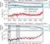 |
Figure 1 Examples of derived mass densities for two debris objects. (a and c) Average orbital altitude in black and orbital eccentricity in blue on the right y-axis. The dashed line shows eccentricity 0.0025, which is later used as an upper limit for the analysis. (b and d) Orbit-averaged mass densities from the JB2008 model in black and derived from TLEs. Gray shading indicates times when the eccentricity is above the chosen limit. The panel titles show object name, international designator (or COSPAR ID), and the catalogue number assigned to the object. |
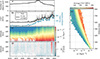 |
Figure 2 Results from deriving atmospheric density from space debris TLEs. (a) Number of objects used over time. (b) Daily and 81-day average of F10.7 in black and the monthly sunspot number in blue on the right axis. (c) Derived mass density as a function of altitude. (d) Ratio between mass density derived from TLEs and given by the JB2008 model. (e) 〈ρ〉 from all TLE pairs as a function of altitude, colored after the average F10.7. Only bins with more than 10 TLE pairs are shown. |
The first object, shown in Figures 1a–1b, is a piece that originates from the 2009 Iridium 33 – Kosmos 2251 collision. It first appeared in the TLE catalogue in July 2009 in a nearly circular orbit at ∼790 km altitude. As the eccentricity is low, we can derive the orbit-averaged density 〈ρ〉 45 days after the initial TLE. The resulting mass density closely tracks the JB2008 values, with larger deviations only at altitudes above ∼700 km.
The second object, shown in Figures 1b–1c, originates from the destructive test of an antisatellite weapon on the Kosmos 1408 satellite. The object first appeared in the TLE catalog in December 2021, roughly one month after the weapons test. Again, the TLE-derived mass densities can be determined 45 days after the initial TLE. Since the method is applicable to circular orbits, we restrict our analysis to eccentricities less than 0.0025 (see Sect. 2.4). Therefore, when the eccentricity is greater than this limit, the method is not suitable for determining 〈ρ〉. These time intervals for the second object are shaded in Figures 1c–1d. In general, our method accurately reproduces the JB2008 model densities using TLE from space debris objects with circular orbits.
2.4 Object selection
A large number of objects are required to obtain the global density profiles of the upper atmosphere (e.g., Emmert, 2009). To avoid including maneuvering satellites, we limit our analysis to objects classified as either debris or rocket bodies by the 18SDS. In this work, we apply the method described above to the years 2018–2024, which constitute the end of solar cycle 24 and roughly the first half of solar cycle 25 (Pesnell, 2020; Interrante, 2024). Therefore, we initially select objects from the US satellite catalog that were in orbit during this period.
We limit our analysis to debris objects in circular, low-Earth orbits, as orbital eccentricity introduces small errors to the derived mass density. However, by assuming circular orbits, the computations do not require atmospheric models or further orbit propagation. We estimate that the main source of uncertainty arising from a small eccentricity is the variable altitude during the orbit. In order to keep this uncertainty low, we only apply equation (4) when the eccentricity ϵ is below 0.0025, which corresponds to less than 10 km variations in geocentric distance in low-Earth orbit. We further limit our analysis to altitudes below 800 km. While previous studies by Emmert (2009) and Emmert et al. (2021a) considered objects below 600 km, we estimate that the method remains reliable above these altitudes. Although uncertainties increase slightly at higher altitudes, as illustrated in Figure 1b, the derived densities remain consistent with model predictions.
Earth’s ellipsoid shape will introduce similar uncertainties as orbital eccentricity in the density profiles. Here we define the altitude of an object’s orbit as the mean geodetic altitude, i.e., the distance from the object to the geoid surface. The ellipsoid shape of Earth, therefore, introduces an intrinsic ambiguity of approximately ±10 km in altitude (Moritz, 2000), which is comparable to the maximum uncertainty from the slightly eccentric orbits.
Finally, we apply several selection criteria to ensure data reliability. First, we limit the fraction of TLE pairs that show an increase, rather than a decay of the orbital altitude. These increases in orbital energy would yield negative mass densities and are due to noise in the TLE data Emmert (2009), since the space debris objects are unable to perform orbit-raising maneuvers. Emmert (2009) previously excluded objects where more than 25% of TLE pairs showed an increase in altitude. Here, we use a stricter 2% limit to keep the noise level in the TLE-derived densities low while still maintaining a relatively large sample size, which assures a better altitude coverage. Second, to exclude objects with unstable or changing aerodynamic properties, we discard objects whose computed βm that exhibit large variations. Large deviations may result from unmodeled effects such as solar radiation pressure or from further fragmentation and collisions. To avoid these effects due to unstable inverse ballistic coefficients and to sort out objects that, for example, undergo fragmentation during the studied interval, we require that both the median and the mean absolute deviation of βm are within 100% of the median value. These criteria ensure that the remaining objects maintain a sufficiently stable βm for reliable thermospheric mass density estimation. In total, 894 objects, or roughly 34% of the objects, were rejected due to either noisy orbits or unstable inverse ballistic coefficients.
The number of objects used in the analysis will naturally vary over time as new debris is generated, orbits circularize, or objects reenter the atmosphere (see Fig. 2a). Over the time period 2018–2024, a total of 2348 separate objects were used. A large proportion of these objects originates from well-known debris-generating events such as the destruction of Fengyun 1C (Johnson et al., 2008), the collision between Iridium 33 and Kosmos 2251 (Pardini & Anselmo, 2023), the breakup of Resurs O1 (Anz-Meador et al., 2023), and, with the largest number of objects originating from the destruction of Kosmos 1408 in November 2021 (e.g., Kastinen et al., 2023).
3 Results
3.1 Derived dataset of globally averaged mass density
We apply the method to obtain a simulated near-real-time, globally averaged mass density profile for the years 2018 to 2024. Figure 2 summarizes the results from this time period. We can see a clear increase in the number of objects used in the analysis following the destruction of Kosmos 1408 in November 2021 in Figure 2a. The number of space debris objects decreases after this as the solar cycle ramps up, as seen in the solar flux F10.7-index and the sunspot number (Clette & Lefèvre, 2015; Clette et al., 2016) in Figure 2b. This is due to an increase in mass density and drag in low-Earth orbits since direct heating from extreme ultraviolet and soft X-rays causes a greater number of objects to reenter the atmosphere. The median time difference between the TLEs in a pair varies between approximately 12 and 20 h during this time period, which means that the data set has a relatively high temporal resolution.
Figure 2c shows the globally averaged mass density profiles over time. These profiles are averages of orbit-averaged mass density values, derived from each TLE pair across all selected debris objects. As the number of contributing objects is large, and because a single orbit typically samples a wide range of latitudes and local times, the individual orbit-averaged densities can be translated into global density profiles (Emmert, 2009). This is achieved by binning the data into equally spaced altitude bins, with edges from 200 to 800 km and widths of 25 km. The bins are selected to be larger than the altitude uncertainties, while also ensuring a sufficient number of TLE pairs in each bin. Other bin-widths produce similar results to those presented here. The time series in each altitude bin is calculated using a Gaussian kernel smoothing. Since the median time resolution of TLE pairs is at best ∼12 h, we set the time resolution to 6 h and the width of the kernel smoothing to ±6 h, in order to ensure that all variations in the mass density data are captured. This timeseries data for 2018–2024 is made available as a supplemental material to this paper.
The computed mass density shows a clear dependence on the solar cycle. Figure 2c shows the globally averaged mass density, using values of βm given by the JB2008 model, as a function of altitude. We see a clear expansion of the thermosphere and an increase in density as solar cycle 25 progressed. Additionally, there is a clear ∼27-day periodicity in the density, corresponding to the solar rotation period and variation in solar flux (Poblet & Azpilicueta, 2018). Figure 2e shows the globally averaged mass density profiles from 2018 to 2024, with the color showing the average F10.7 solar flux index. Similarly, we here see the well-known dependence of mass density in the thermosphere on the solar cycle and solar activity levels (e.g., Walterscheid, 1989).
Since the results are based on inverse ballistic coefficients calculated using the JB2008 model, the computed mass density will, on average, match the model densities, but there are significant differences. This is because TLE-derived densities depend on the orbit evolution of the space objects, with the model densities serving only as a scaling reference through the inverse ballistic coefficients. Figure 2d shows the ratio between the computed from TLE data and modeled densities. First, we see a clear oscillation in the ratio, with a period of one year throughout the time period. This discrepancy corresponds to the annual variation in mass density (Paetzold & Zschörner, 1961). It is possible that the JB2008 model, during this time period, underestimates the mass density during the primary minimum of the seasonal variations, which occurs during the northern hemisphere summer (Qian et al., 2009; Emmert, 2015). This type of variation in the density ratio is less apparent when compared with the NRLMSISE–00 and 2.0 models (not shown).
During a period centered around June 2024, there was a notable discrepancy between the mass density derived from TLEs and the model value. As shown in Figure 2c, the computed densities are significantly higher than the model values, highlighting a limitation of the JB2008 model. There is likely an issue with the solar indices in the data file that is used to compute the model densities (Bruinsma et al., 2018). Since the JB2008 computations for this study were performed in March 2025, this discrepancy may be reduced or eliminated in the future as the solar indices are reprocessed. This highlights the limitations of the chosen underlying model for this method and suggests that alternative models may be more appropriate for future implementations of the method. At the same time, as we shall see in Section 3.2, it also shows a case where the underlying atmospheric model JB2008 significantly underestimates the mass density, while the method described here successfully captures the true density.
Figure 2d also shows the density ratio dependence on altitude. It is clear that there is a trend for lower ratios at altitudes below ∼300 km, as the objects are about to reenter the inner atmosphere. This is likely due to the assumption of constant β, as it does not fully hold at these altitudes. The drag coefficient CD of an object is dependent not just on the shape, but also on the composition, temperature, and density of the surrounding atmosphere (Doornbos, 2011). In general, this dependency leads to a lower CD at lower altitudes (e.g., Moe & Moe, 2005; Vallado & Finkleman, 2014; Walker et al., 2014; Mehta et al., 2023), which in turn leads to the method described here underestimating the mass density as such changes in CD are not modeled. Despite this, the method still correctly models decay rates of objects at these altitudes.
3.2 Validation
To validate and test this method for deriving atmospheric mass density from TLEs in near-real-time, we compare the computed densities to those observed by spacecraft in low-Earth orbit. For this comparison and validation, we use data from the Gravity Recovery and Climate Experiment Follow-on (GRACE-FO) mission (Landerer et al., 2020) as well as from the Swarm mission (Friis-Christensen et al., 2008). These are the two missions with instrumentation that observe the in-situ mass density of the upper atmosphere during the period of this study.
The GRACE-FO mission was launched in 2018 and consists of two satellites separated along-track in a polar orbit at roughly 490 km altitude. We use mass density data derived from the accelerometer instrument (ACC) on board the satellites (Siemes et al., 2023; Hładczuk et al., 2024). The Swarm mission, meanwhile, comprises three satellites: Swarm A and Swarm C, which orbit closely together at approximately 450 km altitude, and Swarm B, which operates at a slightly higher altitude of about 500 km. For Swarm, we use mass density observations derived by estimating the acceleration using precise orbit determination (POD) from GPS data from the spacecraft (March et al., 2019; van den IJssel et al., 2020).
The results of the validation against GRACE-FO measurements are summarized in Figure 3. Specifically, the figure shows the orbit-averaged mass density observed by GRACE-FO and from the JB2008 model, as well as the globally averaged mass density obtained from the TLE data interpolated from its 25-kilometer resolution to the mean altitude of the spacecraft. We see a general agreement between the three time series over the entire period studied here. One exception is the period around July 2024, where JB2008 predicts an unrealistically low density (see discussion in Sect. 3.1). The TLE-derived density, however, successfully captures the values measured by GRACE-FO during this period, as it relies only on historical model densities.
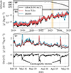 |
Figure 3 Comparison of orbit-averaged densities derived from accelerometer measurements onboard GRACE-FO to the density from space debris TLEs. (a) Average orbital altitude of GRACE-FO. (b) Average densities from GRACE-FO in black, from TLEs in red, and from the JB2008 model in blue. (c) Same as (b) but zoomed in on three geomagnetic storms in 2024. (d) Dst index with the three geomagnetic storms marked with arrows. |
The method also accurately tracks the spacecraft-derived density during geomagnetic storms. Figure 3c shows the densities during a two-week interval where three separate geomagnetic storms occurred (e.g., Dimmock et al., 2024; Pancheva et al., 2024; Li et al., 2025). The first storm measured a G3, and the last two G4 on the NOAA space weather scales Hanslmeier (2002). Figure 3d shows the Dst index (Sugiura, 1963) during these storms and shows clear dips that indicate disturbed geomagnetic storm conditions. As we can see in Figure 3c, the storms cause clear increases in mass density along the orbit of GRACE-FO. During this time, both the JB2008 model and, especially, the density derived from space debris TLEs show excellent agreement with accelerometer data from GRACE-FO. This shows that the method described here can accurately nowcast satellite drag in low-Earth orbit, even during geomagnetic storms.
We now do a more formal validation of the method over a longer time. We compare the mass density derived from TLEs in the method described above with observed densities by the GRACE-FO and Swarm satellites from 2019 to 2024, since GRACE-FO was launched in 2018. Table 1 shows scorecards in the same format used by Bruinsma et al. (2018). The empirical JB2008 and NRLMSISE-00 and 2.0 models are also included for reference and comparison. The spacecraft and model densities are downsampled to the temporal resolution of the dataset described above, of 6 h, but as we discussed earlier, the true temporal resolution of the TLE-derived densities is at best ∼12 h. We can see that, compared to GRACE-FO measurements, the method described here slightly overestimates the mass density with an average (total) observed-to-computed ratio of 0.82 (0.88). The density ratios are naturally close to those of the JB2008 model, since this model is used as a scaling reference. The NRLMSISE models overestimate the density to an even higher degree, as can be seen in Table 1. A similar trend is shown with the Swarm satellites in Table 1. Absolute atmospheric densities are difficult to measure unambiguously and generally rely on assumptions about spacecraft aerodynamic properties or instrument calibration. Models are therefore typically scaled to reference measurements, see Bruinsma et al. (2018). The observed-to-computed density ratios are therefore likely due to differences in the absolute scaling between the data set and models (van den IJssel et al., 2020; Siemes et al., 2023). The absolute density values obtained with this method are dependent on which model is chosen to compute βm, and it is possible that some other models, not tested here, would produce densities that are on average more similar to the satellite measurements.
Average (total) observed-to-computed density ratio, standard deviation [%], and correlation coefficient. Scorecard after Bruinsma et al. (2018) of the calculated densities from TLEs of space debris and empirical models compared to densities observed by the GRACE-FO and Swarm A and B spacecraft. Swarm C is omitted because its values are essentially identical to Swarm A’s.
We now turn to how well the method estimates variations in neutral density caused by space weather and other effects. Table 1, in addition to density ratios, also shows both the standard deviation of the density ratios and the Pearson correlation coefficient between the densities from TLEs and the models (Bruinsma et al., 2018). We can see that the near real-time estimation from the TLE data has significantly lower standard deviations of the density ratio, and, in nearly all cases, a higher correlation coefficient than the three empirical models tested here. When using inverse ballistic coefficients computed with NRLMSISE-00 and 2.0 (not shown), the TLE-derived densities yield similar statistical performance to those shown here that use JB2008, but the density ratios align more closely with the respective model itself. It is therefore clear that the method we present here outperforms these methods in nowcasting of satellite drag on these time-scales.
3.3 Example – May 2024 Geomagnetic storm
Finally, we demonstrate a simple use-case of the method described here during the May 2024 Gannon geomagnetic storm. The geomagnetic storm measured G5 on the NOAA scale and was caused by a number of coronal mass ejections that impacted Earth on May 10–11 (Hajra et al., 2024) and had a significant impacts on satellite orbits and operations (Parker & Linares, 2024).
Figure 4 shows an overview of the storm. Panels a and b show solar wind data from the plasma and magnetic field instruments onboard the Wind spacecraft (Lepping et al., 1995; Ogilvie et al., 1995), which is positioned in the first Lagrange point upstream of Earth. We see that the first interplanetary shock, seen as a sudden increase in solar wind speed, density, and magnetic field strength associated with the coronal mass ejections, reached Wind at around 17:00 UTC on May 10. We see in Figure 4a that the magnetic field in the complex structure of sheath and magnetic cloud plasma, after the initial shock, is predominantly southward with Bz < 0, see (Hajra et al., 2024) for details. This southward field caused the geomagnetic storm, which can be seen in both Dst (Nose et al., 2015) and Hp30, a Kp-like an index with 30-minute resolution that can exceed Kp’s maximum value of 9 (Yamazaki et al., 2022), see Figure 4c.
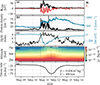 |
Figure 4 Overview of the G5 geomagnetic storm in May 2024 and solar wind observations from the Wind spacecraft. (a) Solar wind magnetic field strength and z-component in the geocentric solar magnetic coordinate system. (b) Solar wind proton density in black and speed on the right axis in blue. (c) Geomagnetic Hp30 index in black and Dst on the right axis in blue. (d) TLE-derived thermospheric mass density as a function of altitude. (e) Orbital decay of a fictional, GRACE-like satellite. The two vertical dashed lines show the arrival of the first interplanetary shock and the time of maximum satellite drag, respectively. |
The geomagnetic storm led to a sharp increase in satellite drag in low-Earth orbit. As shown in Figure 4d, the atmospheric mass density increased at all altitudes during the storm. Figure 4e shows the corresponding rise in the orbital decay rate of a fictional satellite in a circular orbit at 490 km. The decay rate is approximated by  , where the orbit and inverse ballistic coefficient are based on a nominal GRACE-like satellite (Wen et al., 2019), similar to that used by Krauss et al. (2024). We see a clear increase in the mass density at all altitudes and an increase in orbit decay rate greater than a factor of four at 490 km. The greatest level of satellite decay is reached approximately 24 h after the arrival of the initial shock wave, and the enhanced decay rate lasts for approximately 1–2 days, mostly consistent with earlier studies (Oliveira et al., 2017; Oliveira & Zesta, 2019). The decay rate would be difficult to model during the geomagnetic storm, but this method could be used to give a near-real-time estimate of the drag, which would be valuable in satellite operations.
4 Conclusions
In this paper, we present a data-driven, computationally efficient, and operationally feasible method of computing the effects of satellite drag in near-real time. We use TLE tracking data for a large number of space debris objects to infer the mass density in the range of 200–800 km. The method we present is a modified version of existing methods (e.g., Picone et al., 2005; Emmert et al., 2006, 2017), and uses only objects with circular orbits which enables the analysis to be performed without the direct use of atmospheric models, space weather indices, or further orbit propagation, after the object’s inverse ballistic coefficients have been estimated, which makes the method lightweight and suitable for satellite operations.
We implement this method at the end of solar cycle 24 and at the beginning of solar cycle 25 in the years 2018–2024. Using only information that was available at the time of the measurements, we simulate near-real-time atmospheric mass density computations. The dataset is compiled of a total of 2348 objects and readily reproduces the well-known dependence of atmospheric density on solar cycle and activity levels. The median time difference between TLE pairs, and therefore the time resolution of the mass density data, is roughly 12–20 h throughout this period. Combined with an altitude resolution of 25 km, the method captures relevant space-weather processes that affect the decay rate of satellites (Emmert, 2015). The dataset is provided along with this paper.
Validation against spacecraft-derived mass densities shows an excellent performance of the method. The mass density derived from space debris TLEs reproduces the mass density on timescales of days, even during intense geomagnetic storms. Overall, the method showed a better agreement with densities measured by the GRACE-FO and Swarm spacecraft than the JB2008, NRLMSIS–00, and NRLMSIS 2.0 empirical models.
Finally, we demonstrate a simple use-case of the method during the May 2024 Gannon storm. We observe an elevated satellite drag for several days during the storm, with a peak roughly one day after the arrival of the first coronal mass ejection. This information would have been available during the storm, highlighting the potential use of this method to provide timely drag estimations, which is critical for satellite operations and collision risk assessments. Potential future work includes integrating the data from this method with atmospheric models or machine learning, which may extend it to non-circular orbits, and exploring uses for the method in operational space situational awareness.
Acknowledgments
We would like to thank all data providers who made this work possible. This includes the 18SDS for TLE data, the World Data Center for Geomagnetism in Kyoto for the Dst indices, the Dominion Radio Astrophysical Observatory for the F10.7 data, WDC-SILSO, Royal Observatory of Belgium, for the sunspot number data, GFZ Potsdam, for the Hp30 indices, the Wind MFI and SWE instrument teams for the solar wind data, and TU Delft for making the spacecraft-derived mass densities used here publicly available. Density model values were calculated using the pyatmos (Li, 2024) and pymsis (Lucas, 2024) Python packages. The editor thanks Eelco Doornbos and an anonymous reviewer for their assistance in evaluating this paper.
Funding
This work is supported by the Swedish Armed Forces’ Research and Technology Development Programme.
Data availability statement
The orbital data of the debris objects used in this study are available at the United States Space Force’s Space-Track orbital catalog https://www.space-track.org. Space weather input data for the JB2008 model were provided by Space Environment Technologies https://spacewx.com/jb2008/. The Dst indices are provided by the WDC for Geomagnetism, Kyoto, and obtained through the GSFC/SPDF OMNIWeb interface https://omniweb.gsfc.nasa.gov. The sunspot data are provided by WDC-SILSO, Royal Observatory of Belgium, Brussels, and are available through https://www.sidc.be/SILSO/datafiles. The F10.7 solar flux data are recorded at the Dominion Radio Astrophysical Observatory, and provided through https://spaceweather.gc.ca/. The geomagnetic Hp 30 data are provided by GFZ Potsdam and are available through https://kp.gfz-potsdam.de/en/. Solar wind data from Wind are available from https://wind.nasa.gov/. Swarm and GRACE-FO density are available through http://thermosphere.tudelft.nl/.
Supplementary material
Supplementary File 1: Orbit-averaged mass densities calculated from TLEs. The file is in json format and contains values as well as standard deviations of the atmospheric mass density as a function of time and geodetic altitude. Access Supplementary Material
References
- Anz-Meador P, Opiela Jacobs J, Liou JC. 2023. History of on-orbit satellite fragmentations. (16th edn). Technical Publication. NASA/TP-20220019160, Orbital Debris Program Office, National Aeronautics and Space Administration, Lyndon B. Johnson Space Center: Houston, TX. https://ntrs.nasa.gov/citations/20220019160. [Google Scholar]
- Baker D. 2000. The occurrence of operational anomalies in spacecraft and their relationship to space weather. IEEE Trans Plasma Sci 28(6): 2007–2016. [Google Scholar]
- Berger TE, Dominique M, Lucas G, Pilinski M, Ray V, Sewell R, Sutton EK, Thayer JP, Thiemann E. 2023. The thermosphere is a drag: The 2022 starlink incident and the threat of geomagnetic storms to low earth orbit space operations. Space Weather 21(3): e2022SW003330. [CrossRef] [Google Scholar]
- Berger TE, Holzinger MJ, Sutton EK, Thayer JP. 2020. Flying through uncertainty. Space Weather 18(1): e2019SW002373. [Google Scholar]
- Bowman BW, Tobiska K, Marcos F, Huang C, Lin C, Burke W. 2008. A new empirical thermospheric density model JB2008 using new solar and geomagnetic indices AIAA 2008-6438. In: AIAA/AAS Astrodynamics Specialist Conference and Exhibit. American Institute of Aeronautics and Astronautics. https://doi.org/10.2514/6.2008-6438. [Google Scholar]
- Bruinsma S. 2015. The DTM-2013 thermosphere model. J Space Weather Space Clim 5: A1. [CrossRef] [EDP Sciences] [Google Scholar]
- Bruinsma S, Boniface C. 2021. The operational and research DTM-2020 thermosphere models. J Space Weather Space Clim 11: 47. [CrossRef] [EDP Sciences] [Google Scholar]
- Bruinsma S, Sutton E, Solomon SC, Fuller-Rowell T, Fedrizzi M. 2018. Space weather modeling capabilities assessment: neutral density for orbit determination at low earth orbit. Space weather 16(11): 1806–1816. [Google Scholar]
- Bussy-Virat CD, Ridley AJ, Getchius JW. 2018. Effects of uncertainties in the atmospheric density on the probability of collision between space objects. Space Weather 16(5): 519–537. [Google Scholar]
- Buzulukova N, Tsurutani B. 2022. Space weather: from solar origins to risks and hazards evolving in time. Front Astron Space Sci 9: 1017103. [Google Scholar]
- Clette F, Cliver EW, Lefèvre L, Svalgaard L, Vaquero JM, Leibacher JW. 2016. Preface to topical issue: recalibration of the sunspot number. Solar Phys 291: 2479–2486. [Google Scholar]
- Clette F, Lefèvre L. 2015. SILSO sunspot number V2.0. WDC SILSO. Royal Observatory of Belgium (ROB). https://doi.org/10.24414/qnza-ac80. [Google Scholar]
- Dhadly M, Sassi F, Emmert J, Drob D, Conde M, Wu Q, Makela J, Budzien S, Nicholas A. 2023. Neutral winds from mesosphere to thermosphere – past, present, and future outlook. Front Astron Space Sci 9: 1050586. [Google Scholar]
- Dimmock AP, Lanabere V, Johlander A, Rosenqvist L, Yordanova E, Buchert S, Molenkamp S, Setréus J. 2024. Investigating the trip of a transformer in Sweden during the 24 April 2023 storm. Space Weather 22(11): e2024SW003948. [Google Scholar]
- Doornbos E, Bruinsma S, Pilinski MD, Bowman B. 2013. The need for a standard for satellite drag computation to improve consistency between thermosphere density models and data sets. In: Proceedings of the 6th European Conference on Space Debris – ESA SP-723. Darmstadt, Germany: ESA Space Debris Office. Available at https://conference.sdo.esoc.esa.int/proceedings/sdc6/paper/130. [Google Scholar]
- Doornbos EN. 2011. Thermospheric density and wind determination from satellite dynamics. Ph.D. Thesis, Delft University of Technology. [Google Scholar]
- Emmert JT. 2009. A long-term data set of globally averaged thermospheric total mass density. J Geophys Res Space Phys 114(A6): A06315. [Google Scholar]
- Emmert JT. 2015. Thermospheric mass density: a review. Adv Space Res 56(5): 773–824. [CrossRef] [Google Scholar]
- Emmert JT, Dhadly MS, Segerman AM. 2021a. A globally averaged thermospheric density data set derived from two-line orbital element sets and special perturbations state vectors. J Geophys Res Space Phys 126(8): e2021JA029,455. [Google Scholar]
- Emmert JT, Drob DP, Picone JM, Siskind DE, Jones M Jr., et al. 2021b. NRLMSIS 2.0: a whole-atmosphere empirical model of temperature and neutral species densities. Earth Space Sci 8(3): e2020EA001321. [Google Scholar]
- Emmert JT, Meier RR, Picone JM, Lean JL, Christensen AB. 2006. Thermospheric density 2002–2004: TIMED/GUVI dayside limb observations and satellite drag. J Geophys Res Space Phys 111(A10): A10S16. [Google Scholar]
- Emmert JT, Warren HP, Segerman AM, Byers JM, Picone JM. 2017. Propagation of atmospheric density errors to satellite orbits. Adv Space Res 59(1): 147–165. [CrossRef] [Google Scholar]
- Friis-Christensen E, Lühr H, Knudsen D, Haagmans R. 2008. Swarm–an earth observation mission investigating geospace. Adv Space Res 41(1): 210–216. [CrossRef] [Google Scholar]
- Fuller-Rowell T, Solomon SC. 2010. Flares, coronal mass ejections, and atmospheric responses. In: Heliophysics: space storms and radiation: causes and effects, Siscoe GL, Schrijver CJ (Eds.) Cambridge: Cambridge University Press, pp. 321–358. [Google Scholar]
- Geul J, Mooij E, Noomen R. 2017. Assessment and modelling of space surveillance network. In: Proceedings of the 7th European Conference on Space Debris. Darmstadt, Germany: ESA Space Debris Office. https://conference.sdo.esoc.esa.int/proceedings/sdc7/paper/1014. [Google Scholar]
- Hajra R, Tsurutani BT, Lakhina GS, Lu Q, Du A. 2024. Interplanetary causes and impacts of the 2024 May superstorm on the geosphere: an overview. Astrophys J 974(2): 264. [Google Scholar]
- Hanslmeier A. 2002. The NOAA space weather scales. Dordrecht: Springer Netherlands. ISBN 978-0-306-48211-3. [Google Scholar]
- Hedin AE, Biondi MA, Burnside RG, Hernandez G, Johnson RM, et al.. 1991. Revised global model of thermosphere winds using satellite and ground-based observations. J Geophys Res Space Phys 96(A5): 7657–7688. [Google Scholar]
- Hejduk MD, Casali SJ, Cappellucci DA, Ericson NL, Snow DE. 2013. A catalogue-wide implementation of general perturbations orbit determination extrapolated from higher-order theory solutions–AAS 13–240. In: Proceedings of the AAS/AIAA Space Flight Mechanics Meeting, Kauai, HI. [Google Scholar]
- Hejduk MD, Snow DE. 2018. The effect of neutral density estimation errors on satellite conjunction serious event rates. Space Weather 16(7): 849–869. [CrossRef] [Google Scholar]
- Hładczuk NA, van den Ijssel JKodikara T, Siemes C, Visser P. 2024. GRACE-FO radiation pressure modelling for accurate density and crosswind retrieval. Adv Space Res 73(5): 2355–2373. [CrossRef] [Google Scholar]
- Hoots FR, Roehrich RL. 1980. Models for propagation of NORAD element sets. Fort Belvoir, VA: Defense Technical Information Center. https://doi.org/10.21236/ADA093554. [Google Scholar]
- Interrante AA. 2024. NASA, NOAA announce that the sun has reached the solar maximum period. NASA Scientific Visualization Studio. [Google Scholar]
- Johnson NL, Stansbery E, Liou JC, Horstman M, Stokely C, Whitlock D. 2008. The characteristics and consequences of the break-up of the Fengyun-1C spacecraft. Acta Astronaut 63: 128–135. [Google Scholar]
- Kastinen D, Vierinen J, Grydeland T, Kero J. 2023. Using radar beam-parks to characterize the Kosmos-1408 fragmentation event. Acta Astronaut 202: 341–359. [Google Scholar]
- Kessler DJ, Cour-Palais BG. 1978. Collision frequency of artificial satellites: the creation of a debris belt. J Geophys Res Space Phys 83(A6): 2637–2646. [Google Scholar]
- King-Hele DG. 1987. Satellite orbits in an atmosphere: theory and applications (1st edn). Dordrecht: Springer. ISBN 978-0-216-92252-5. [Google Scholar]
- Krauss S, Drescher L, Temmer M, Suesser-Rechberger B, Strasser A, Kroisz S. 2024. SODA – a tool to predict storm-induced orbit decays for low earth-orbiting satellites. J Space Weather Space Clim 14: 23. [Google Scholar]
- Landerer FW, Flechtner FM, Save H, Webb FH, Bandikova T, et al. 2020. Extending the global mass change data record: GRACE follow-on instrument and science data performance. Geophys Res Lett 47(12): e2020GL088306. [CrossRef] [Google Scholar]
- Lepping RP, Acũna MH, Burlaga LF, Farrell WM, Slavin JA, et al. 1995. The WIND magnetic field investigation. Space Sci Rev 71(1): 207–229. [CrossRef] [Google Scholar]
- Li C. 2024. Python package–Pyatmos 1.2.7. Available at https://github.com/lcx366/ATMOS. [Google Scholar]
- Li T, Zheng D, He C, Ye F, Yuan P, Yao Y, Liao M, Xie J. 2025. Ionospheric response to the 24–27 February 2023 solar flare and geomagnetic storms over the European region using a machine learning-based tomographic technique. Space Weather 23(1): e2024SW004146. [Google Scholar]
- Licata RJ, Mehta PM. 2023. Reduced order probabilistic emulation for physics-based thermosphere models. Space Weather 21(5): e2022SW003345. [Google Scholar]
- Lilensten J, Dudok de Wit T, Kretzschmar M, Amblard P-O, Moussaoui S, Aboudarham J, Auchère F. 2008. Review on the solar spectral variability in the EUV for space weather purposes. Ann Geophys 26(2): 269–279. [Google Scholar]
- Lucas G. 2024. Python package–Pymsis. Zenodo. https://doi.org/10.5281/zenodo.14188070. [Google Scholar]
- March G, Doornbos EN, Visser PNAM. 2019. High-fidelity geometry models for improving the consistency of CHAMP, GRACE, GOCE and Swarm thermospheric density data sets. Adv Space Res 63(1): 213–238. [CrossRef] [Google Scholar]
- Mehta PM, Licata RJ. 2025. TIE-GCM ROPE–Dimensionality reduction: Part I. Space Weather 23(1): e2024SW004,185. [Google Scholar]
- Mehta PM, Paul SN, Crisp NH, Sheridan PL, Siemes C, March G, Bruinsma S. 2023. Satellite drag coefficient modeling for thermosphere science and mission operations. Adv Space Res 72(12): 5443–5459. [Google Scholar]
- Moe K, Moe MM. 2005. Gas–surface interactions and satellite drag coefficients. Planet Space Sci . 53 (8): 793–801. [Google Scholar]
- Moritz H. 2000. Geodetic reference system 1980. J Geodesy . 74 (1): 128–133. [Google Scholar]
- Mutschler SM, Axelrad P, Sutton EK, Masters D. 2023. Physics-based approach to thermospheric density estimation using CubeSat GPS data. Space Weather 21(1): e2021SW002997. [Google Scholar]
- Nose M, Sugiura M, Kamei T, Iyemori T, Koyama Y. 2015. Dst index. Kyoto: World Data Center for Geomagnetism. https://doi.org/10.17593/14515-74000. [Google Scholar]
- Ogilvie KW, Chornay DJ, Fritzenreiter RJ, Hunsaker F, Keller J. et al. 1995. SWE, a comprehensive plasma instrument for the wind spacecraft. Space Sci Rev. 71 (1): 55–77. [CrossRef] [Google Scholar]
- Oliveira DM, Zesta E. 2019. Satellite orbital drag during magnetic storms. Space Weather 17(11): 1510–1533. [CrossRef] [Google Scholar]
- Oliveira DM, Zesta E, Schuck PW, Sutton EK. 2017. Thermosphere global time response to geomagnetic storms caused by coronal mass ejections. J Geophys Res Space Phys 122(10): 10762–10782. [Google Scholar]
- Oltrogge D, Ramrath J. 2014. Parametric characterization of SGP4 theory and TLE positional accuracy. in: Advanced Maui Optical and Space Surveillance Technologies Conference, E87. Available at https://amostech.com/TechnicalPapers/2014/Poster/OLTROGGE.pdf. [Google Scholar]
- Paetzold HK, Zschörner H. 1961. An annual and a semiannual variation of the upper air density. Geofisica Pura Applicata 48(1): 85–92. [Google Scholar]
- Pancheva D, Mukhtarov P, Bojilova R. 2024. Response to geomagnetic storm on 23–24 March 2023 long-lasting longitudinal variations of the global ionospheric TEC. Adv Space Res 73(12): 6006–6028. [Google Scholar]
- Pardini C, Anselmo L. 2023. The short-term effects of the cosmos 1408 fragmentation on neighboring inhabited space stations and large constellations. Acta Astronaut 210: 465–473. [Google Scholar]
- Parker WE, Linares R. 2024. Satellite drag analysis during the May 2024 gannon geomagnetic storm. J Spacecr Rockets 61(5): 1412–1416. [Google Scholar]
- Pesnell WD. 2020. Lessons learned from predictions of solar cycle 24. J Space Weather Space Clim 10: 60. [Google Scholar]
- Picone JM, Emmert JT, Lean JL. 2005. Thermospheric densities derived from spacecraft orbits: accurate processing of two-line element sets. J Geophys Res Space Phys 110(A3): A03301. [Google Scholar]
- Picone JM, Hedin AE, Drob DP, Aikin AC. 2002. NRLMSISE-00 empirical model of the atmosphere: statistical comparisons and scientific issues. J Geophys Res Space Phys 107(A12): SIA 15–1–SIA 15–16. [Google Scholar]
- Poblet FL, Azpilicueta F. 2018. 27-day variation in solar-terrestrial parameters: global characteristics and an origin based approach of the signals. Adv Space Res 61(9): 2275–2289. [Google Scholar]
- Pulkkinen T. 2007. Space weather: terrestrial perspective. Living Rev Solar Phys 4(1): 1. [CrossRef] [Google Scholar]
- Qian L, Burns AG, Emery BA, Foster B, Lu G, Maute A, Richmond AD, Roble RG, Solomon SC, Wang W. 2014. The NCAR TIE-GCM. In: Chapter 7: Modeling the ionosphere – thermosphere system. American Geophysical Union, pp. 73–83. ISBN 978-1-118-70441-7. https://doi.org/10.1002/9781118704417.ch7. [Google Scholar]
- Qian L, Solomon SC, Kane TJ. 2009. Seasonal variation of thermospheric density and composition. J Geophys Res Space Phys 114(A1): A01312. [CrossRef] [Google Scholar]
- Siemes C, Borries C, Bruinsma S, Fernandez-Gomez I, Hładczuk N, den Ijssel J, Kodikara T, Vielberg K, Visser P. 2023. New thermosphere neutral mass density and crosswind datasets from CHAMP, GRACE, and GRACE-FOJ Space Weather Space Clim 13: 16. [CrossRef] [EDP Sciences] [Google Scholar]
- Sridharan R, Pensa AF. 1998. U.S. space surveillance network capabilities. Proc SPIE 3434: 88–100. [Google Scholar]
- Storz MF, Bowman BR, Branson MJI, Casali SJ, Tobiska WK. 2005. High accuracy satellite drag model (HASDM). Adv Space Res 36(12): 2497–2505. [Google Scholar]
- Sugiura M. 1963. Hourly values of equatorial Dst for the IGY. Ann Int Geophys Year 35: 9–45. [Google Scholar]
- Sutton EK. 2018. A new method of physics-based data assimilation for the quiet and disturbed thermosphere. Space Weather 16(6): 736–753. [CrossRef] [Google Scholar]
- Tapping KF. 2013. The 10.7 Cm solar radio flux (F10.7). Space Weather 11(7): 394–406. [CrossRef] [Google Scholar]
- Thayer JP, Tobiska WK, Pilinski MD, Sutton EK. 2021. Chapter 5: Remaining issues in upper atmosphere satellite drag. In: Space weather effects and applications. American Geophysical Union, pp. 111–140. ISBN 978-1-119-81557-0. https://doi.org/10.1002/9781119815570.ch5. [Google Scholar]
- Vallado DA, Finkleman D. 2014. A critical assessment of satellite drag and atmospheric density modeling. Acta Astronaut 95: 141–165. [CrossRef] [Google Scholar]
- van den IJssel J, Doornbos E, Iorfida E, March G, Siemes C, Montenbruck O. 2020. Thermosphere densities derived from swarm GPS observations. Adv Space Res 65(7): 1758–1771. [CrossRef] [Google Scholar]
- WalkerA, Mehta P, Koller J. 2014. Drag coefficient model using the Cercignani–Lampis–Lord gas–surface interaction model. J Spacecr Rockets 51(5): 1544–1563. [CrossRef] [Google Scholar]
- Walterscheid RL. 1989. Solar cycle effects on the upper atmosphere – implications for satellite drag. J Spacecr Rockets 26(6): 439–444. [Google Scholar]
- Wen HY, Kruizinga G, Paik M, Landerer F, Bertiger W, Sakumura C, Bandikova T, Mccullough C. 2019. Gravity recovery and climate experiment follow-on (GRACE-FO) level-1 data product user handbook. Technical Report JPL D-56935 (URS270772), NASA Jet Propulsion Laboratory, California Institute of Technology. [Google Scholar]
- Yamazaki Y, Matzka J, Stolle C, Kervalishvili G, Rauberg J, Bronkalla O, Morschhauser A, Bruinsma S, Shprits YY, Jackson DR. 2022. Geomagnetic activity index HPO. Geophys Res Lett 49(10): e2022GL098860. [CrossRef] [Google Scholar]
Cite this article as: : Johlander A, Papadogiannakis S & Rasmusson O. 2026. Thermospheric mass density derived in near real time from space debris. J. Space Weather Space Clim. 16, 7. https://doi.org/10.1051/swsc/2026005.
All Tables
Average (total) observed-to-computed density ratio, standard deviation [%], and correlation coefficient. Scorecard after Bruinsma et al. (2018) of the calculated densities from TLEs of space debris and empirical models compared to densities observed by the GRACE-FO and Swarm A and B spacecraft. Swarm C is omitted because its values are essentially identical to Swarm A’s.
All Figures
|
Figure 1 Examples of derived mass densities for two debris objects. (a and c) Average orbital altitude in black and orbital eccentricity in blue on the right y-axis. The dashed line shows eccentricity 0.0025, which is later used as an upper limit for the analysis. (b and d) Orbit-averaged mass densities from the JB2008 model in black and derived from TLEs. Gray shading indicates times when the eccentricity is above the chosen limit. The panel titles show object name, international designator (or COSPAR ID), and the catalogue number assigned to the object. |
| In the text | |
|
Figure 2 Results from deriving atmospheric density from space debris TLEs. (a) Number of objects used over time. (b) Daily and 81-day average of F10.7 in black and the monthly sunspot number in blue on the right axis. (c) Derived mass density as a function of altitude. (d) Ratio between mass density derived from TLEs and given by the JB2008 model. (e) 〈ρ〉 from all TLE pairs as a function of altitude, colored after the average F10.7. Only bins with more than 10 TLE pairs are shown. |
| In the text | |
|
Figure 3 Comparison of orbit-averaged densities derived from accelerometer measurements onboard GRACE-FO to the density from space debris TLEs. (a) Average orbital altitude of GRACE-FO. (b) Average densities from GRACE-FO in black, from TLEs in red, and from the JB2008 model in blue. (c) Same as (b) but zoomed in on three geomagnetic storms in 2024. (d) Dst index with the three geomagnetic storms marked with arrows. |
| In the text | |
|
Figure 4 Overview of the G5 geomagnetic storm in May 2024 and solar wind observations from the Wind spacecraft. (a) Solar wind magnetic field strength and z-component in the geocentric solar magnetic coordinate system. (b) Solar wind proton density in black and speed on the right axis in blue. (c) Geomagnetic Hp30 index in black and Dst on the right axis in blue. (d) TLE-derived thermospheric mass density as a function of altitude. (e) Orbital decay of a fictional, GRACE-like satellite. The two vertical dashed lines show the arrival of the first interplanetary shock and the time of maximum satellite drag, respectively. |
| In the text | |
Current usage metrics show cumulative count of Article Views (full-text article views including HTML views, PDF and ePub downloads, according to the available data) and Abstracts Views on Vision4Press platform.
Data correspond to usage on the plateform after 2015. The current usage metrics is available 48-96 hours after online publication and is updated daily on week days.
Initial download of the metrics may take a while.