| Issue |
J. Space Weather Space Clim.
Volume 16, 2026
Topical Issue - Severe space weather events of May 2024 and their impacts
|
|
|---|---|---|
| Article Number | 6 | |
| Number of page(s) | 16 | |
| DOI | https://doi.org/10.1051/swsc/2025059 | |
| Published online | 02 March 2026 | |
Research Article
LOFAR uniqueness under extreme ionospheric conditions: The May 2024 Mother’s Day superstorm
1
Istituto Nazionale di Geofisica e Vulcanologia, Via di Vigna Murata 605, 00143 Rome, Italy
2
Physics and Astronomy Department “Augusto Righi”, University of Bologna, Via Zamboni 33, 40126 Bologna, Italy
3
SpacEarth Technology, Viale dell’Astronomia 18, 00144 Rome, Italy
4
Space Environment and Radio Engineering (SERENE) research group, University of Birmingham, Edgbaston, Birmingham, B15 2TT, UK
5
ASTRON – The Netherlands Institute for Radio Astronomy, Oude Hoogeveensedijk 4, 7991 PD Dwingeloo, The Netherlands
6
Space Radio-Diagnostics Research Centre, University of Warmia and Mazury, ul. Romana Prawochenskiego 9, 10-719 Olsztyn, Poland
7
Center for Solar-Terrestrial Research, New Jersey Institute of Technology, Newark, NJ 07102, USA
8
Department of Electronic and Electrical Engineering, University of Bath, Claverton Down, Bath, BA2 7AY, UK
9
Centrum Badań Kosmicznych Polskiej Akademii Nauk, Bartycka 18 A, 00-716 Warsaw, Poland
10
Riga Technical University, 6A Kipsalas Street, Rīga, LV-1048, Latvia
11
Ventspils University of Applied Sciences, Engineering Research Institute “Ventspils International Radio Astronomy Center”, Ventspils, LV-3601, Latvia
* Corresponding author: This email address is being protected from spambots. You need JavaScript enabled to view it.
Received:
23
May
2025
Accepted:
18
December
2025
Abstract
The May 2024 Mother’s Day superstorm, the strongest since November 2003, triggered significant ionospheric disturbances. Indeed, during the superstorm, the ionosphere above Europe was transformed into a severely depleted, super-high-altitude plasma structure extending beyond 1500 km above Earth’s surface. We highlight the unique contributions of the LOw Frequency ARray (LOFAR) to ionospheric weather research on this extreme event. Originally designed for radio astronomy, LOFAR’s extensive European network of 52 stations and wide-band capabilities enable high-resolution ionospheric monitoring at both local and regional scales. Leveraging LOFAR measurements, we characterise a plethora of ionospheric effects that occurred during the main and early recovery phases of the storm. We did this by observing significant signal fading associated with the equatorward expansion of the auroral oval during the main phase and by capturing high-speed moving ionospheric irregularities (up to ~800 m/s), and quantifying extreme ionospheric uplift (up to 1500 km) under conditions where conventional HF instruments were not usable due to the occurrence of D-layer absorption, ionospheric G-conditions and uplift above ionosonde altitude range. In this investigation, we harness the unique capabilities of LOFAR to direct view into the structure and dynamics of the ionosphere under the most extreme space weather conditions. Our results confirm LOFAR as an insightful instrument for ionospheric research, offering critical capabilities for advancing storm impact assessment, forecasting, and mitigation strategies.
Key words: LOFAR / Mid-latitude ionosphere / Extreme geomagnetic storm / Ionospheric radio propagation
© R. Ghidoni et al., Published by EDP Sciences 2026
 This is an Open Access article distributed under the terms of the Creative Commons Attribution License (https://creativecommons.org/licenses/by/4.0), which permits unrestricted use, distribution, and reproduction in any medium, provided the original work is properly cited.
1 Introduction
In May 2024, several X-class solar flares originating from Active Region (AR) 13664 triggered multiple coronal mass ejections (CMEs) (Romano et al., 2024; Ippolito et al., 2025). These events culminated on May 10th–11th in the most significant geomagnetic storm since those observed in late 2003, hereafter referred to as the May 2024 Mother’s Day Superstorm (Spogli et al., 2024; Elvidge & Themens, 2025; Jin et al., 2025), following the name convention which has been mostly used in Europe (Chabanski et al., 2025). Classified as an extreme G5-level geomagnetic storm, it was marked by the Kp index reaching its maximum value of 9 for a sustained period, a Dst index drop to −412 nT, and a SYM-H index minimum of −518 nT (Tulasi Ram et al., 2024). While the storm’s peak intensity was estimated as a 1-in-12.5-year event, its prolonged duration, with Kp exceeding 8 for at least 24 h, was exceptionally rare, corresponding to a 1-in-41-year event (Elvidge & Themens, 2025).
This superstorm triggered vast disturbances at the global level, including widespread auroras seen at unusually low latitudes (Foster et al., 2024; Kataoka et al., 2024; Spogli et al., 2024; Chernyshov et al., 2025; Elvidge & Themens, 2025) and significant impacts on the ionosphere-thermosphere system (Themens et al., 2024; Tulasi Ram et al., 2024; Ranjan et al., 2024; Jin et al., 2025).
In the European sector, the storm prompted dramatic ionospheric disturbances, including fast-moving TEC enhancements, equatorward expansion of the auroral oval, poleward expansion of the Northern crest of the Equatorial Ionospheric Anomaly (EIA), and intense ionospheric scintillation phenomena triggered by ionospheric irregularities across a large range of scales.
Specifically, both in situ satellite measurements and ground-based Global Navigation Satellite System (GNSS) observations revealed a significant and rapid depletion of plasma density across high-to-mid latitudes (above 50° magnetic latitude) starting shortly after the storm onset (Jin et al., 2025). This plasma density depletion has been found to be prominent over the Mediterranean sector and Italy (Spogli et al., 2024), originating from a significant ionospheric trough and polar holes and expanded equatorward, lasting for approximately three days before recovering (Jin et al., 2025). This negative ionospheric storm phase is largely attributed to thermospheric composition changes, specifically a decrease in the [O]/[N2] ratio driven by storm-time heating and circulation changes (Spogli et al., 2024; Jin et al., 2025). The depletion was so severe that the F2-layer was effectively absent over high latitudes on May 11th (Themens et al., 2024) and decreased by about 70% with respect to quiet conditions over the Italian mid-latitudes (Spogli et al., 2024). As highlighted by Pierrard et al. (2025), the observed plasma depletion is likely attributable not only to reduced ionization within the F2 layer but also to a contracted plasmapause position. This interpretation supports the hypothesis that the pronounced electron density depletion is associated with plasmaspheric erosion processes.
In the initial storm phases, substantial plasma lifting occurred within the Storm Enhanced Density (SED) plume, with ionospheric peak heights (hmF2) increasing by 150–300 km, reaching up to 630 km over mid-latitudes in the American sector (Themens et al., 2024). Similar hmF2 increases were noted over Italy (Spogli et al., 2024). It has also been reported at low latitudes because of the prompt penetration of electric fields of magnetospheric origin (Fagundes et al., 2025) following the strongly undershielding conditions of the Region 1 and Region 2 Field Aligned Currents at the Interplanetary CME shock arrival (Wei et al., 2015). This lifting contributed to initially enhanced plasma densities before the depletion phase dominated.
In this context, the extensive network of radio telescopes termed LOFAR(van Haarlem et al., 2013) provides the precious opportunity to investigate the ionospheric response, focusing on the severely depleted, super-high-altitude plasma structuring found in Europe.
Recently, LOFAR capabilities have extended beyond astronomy, generating considerable interest in its potential to probe the Earth’s ionosphere (see, e.g. Mevius et al., 2016; Fallows et al., 2020). LOFAR has made significant contributions to ionospheric physics. Boyde et al. (2022) used LOFAR to infer the presence of a small-scale Travelling Ionospheric Disturbance (TID) in the terrestrial ionosphere. The ionospheric effects of plasma structures associated with a medium-scale TID (MSTID), substructure within such a feature, and variations within a sporadic-E layer were reported by Dorrian et al. (2023), Trigg et al. (2024), and Wood et al. (2024), respectively. The effects of multiple TIDs that occurred simultaneously are reported by Fallows et al. (2020). A statistical study (Boyde et al., 2025) has shown that the ionospheric waves are primarily directed in the opposite direction to the prevailing wind, suggesting that they result from quasi-vertically propagating Atmospheric Gravity Waves (AGWs). LOFAR has also been used, often in conjunction with companion datasets like those provided by GNSS measurements, to unveil the physics lying below the formation of ionospheric irregularities (Forte et al., 2022; Flisek et al, 2023) and their dynamics (Grzesiak et al., 2022; Ghidoni et al., 2024).
This study underscores the exceptional capability of LOFAR to capture ionospheric dynamics through high-band antenna observations. For the first time, LOFAR revealed intense scintillation caused by tenuous F-region “bubbles”, capturing fast-moving irregularities (~800 m/s) and quantifying extreme ionospheric uplifting during a period when conventional HF instruments were inoperable, providing a direct view into the structure and dynamics of the ionosphere under the most extreme space weather conditions.
The paper is structured as follows. Section 2 describes the LOFAR data and companion datasets, along with the velocity estimation techniques and the method for deriving an effective ionospheric altitude; Section 3 presents and discusses the key observational results, in particular during the main and recovery phases of the storm, focusing on the high-speed moving irregularities and extreme uplift. Finally, Section 4 provides the concluding remarks.
2 Data and methods
This section introduces the LOFAR data and the related methods to calculate plasma drift velocities and the effective altitude of the ionospheric irregularity (Sect. 2.1), and the companion datasets (Sect. 2.2) to complement LOFAR-based observations: GNSS receivers, ionosondes, and magnetometers.
2.1 LOFAR data
The locations of the LOFAR antennas across Europe are reported in Figure 1. Panel a) shows the locations of the International Stations (IS, red dots), along with the magnetometers of the International Monitor for Auroral Geomagnetic Effects (IMAGE) networks (Tanskanen, 2009) (blue dots) and European ionosondes (green dots). Panel b) shows the position of the Remote Stations (RS), and panel c) illustrates the positions of the Core Stations (CS), which are key to some of our analysis methods.
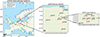 |
Figure 1 Location of LOFAR antennas. Panel a) shows the position of International stations (red dots), IMAGE magnetometers (blue dots), and Ionosondes (green dots). Panel b) shows the position of Remote stations, and panel c) shows the position of Core stations. |
During the May 2024 Mother’s Day superstorm, LOFAR was performing various standard interferometric observations for radio astronomical purposes either with the low band antennas (LBA: 10–90 MHz) or with the high band antennas (HBA: 110–190 MHz). The solar and ionospheric activity during geomagnetic storms makes it difficult to interpret the data for astronomical sciences. However, the station autocorrelations of bright sources show rapid flux amplitude variations due to ionospheric scintillation and can and have therefore been used to study the ionosphere (e.g. Fallows et al., 2020; Flisek et al., 2023; Wood et al., 2024; Ghidoni et al., 2024).
Every LOFAR dataset contains the intensity of the signal coming from the source selected for the observation, measured by every antenna. Data are at a 1-second temporal resolution and at a 0.195 MHz frequency resolution.
Among the LOFAR observations, we also utilise the Incremental Development of LOFAR Space Weather (IDOLS) dataset1. IDOLS represents a unique operational mode within LOFAR’s ionospheric monitoring capabilities, in which a single LOFAR core station (CS032LBA) collects high-resolution intensity data continuously over extended time periods. This setup enables long-duration tracking of ionospheric activity at a fixed location for space weather purposes, offering an uninterrupted view of scintillation and signal variability throughout the storm’s evolution.
The period of available LOFAR observations, along with the K-index from the Dourbes magnetometer and the electrojet indicators IE, IL, and IU derived by IMAGE magnetometers, are shown in Figure 2 and summarized in Table 1.
 |
Figure 2 Panel a) shows the K-index from Dourbes from 15:00 UT on May 9th until 02:00 UT on May 14th. The color of the bars indicates the NOAA Space Weather Scale for geomagnetic storms4. Panel b) shows the electrojet indicators IE, IL, and IU for IMAGE magnetometers. The grey bars represent the five all-stations LOFAR observations, while the blue one represent the period of available IDOLS data. |
Details of the LOFAR observations employed in the analysis. The table provides the associated letter code for each observation, as reported in Figure 2, the LOFAR observation ID, the observed celestial radio source, the antenna type used (LBA or HBA), and the start and end times (UTC) for each observation period.
2.1.1 Dynamic spectra and S4
To remove the slow variations of signal intensity due to non-ionospheric origin, a normalisation algorithm is applied to the dynamic spectra of LOFAR amplitude recorded by each HBA and LBA. A running median filter is applied independently to each frequency channel. The window size for the median filter is 30 min, which suppresses slow variations in the received signal power.
In addition to the normalised dynamic spectra, we calculate the amplitude scintillation index (S4) (Fremouw et al., 1978; Yeh & Liu, 1982), a measure of signal intensity variations:
 (1)
(1)
where I represent the normalized signal intensity, and < … > indicates the mean value over the considered interval. While the GNSS ionospheric community commonly calculates S4 over 60-second intervals, we employ a 180-second window chosen to ensure the calculation interval exceeds the typical cycle period of the observed scintillation variations (Wood et al., 2024).
It is noteworthy that the system noise is neglected in this formula. For very bright sources like Cassiopeia A, the system equivalent flux density can be neglected, but this is not necessarily the case for every 3C source.
S4 intensifies in the presence of ionospheric irregularities smaller than the Fresnel scale for a given wavelength/frequency and observational geometry. LOFAR operates in the HF/VHF band, allowing it to probe irregularities on the order of a few kilometres (see, e.g. Ghidoni et al., 2024). The scale dependence of S4 in LOFAR observations is primarily governed by the Fresnel scale, which determines the dominant irregularity size responsible for scintillation at a given frequency.
2.1.2 Velocity based on cross-correlation
Using LOFAR CSs, it is possible to estimate the velocity of ionospheric irregularities passing across the field of view of the antennas (Fallows et al., 2020). Specifically, from the normalised power measured at a specific frequency by each antenna, the velocity can be expressed in the following form:
 (2)
(2)
where B represents the matrix of distances between the Ionospheric Pierce Points (IPPs) of every couple of LOFAR core stations, while T is a vector containing the time lag between the signals of every pair of antennas. The element (i, j) of matrix B represents the distance between each IPP of station i at the time we are calculating the lag and station j at the time we are calculating the lag plus the lag.
For HBA observations, the velocity of ionospheric irregularities was determined using data at 140 MHz. This frequency was selected to mitigate potential noise introduced by instrument limitations at the boundaries of the available frequency range (110–190 MHz), allowing for a clearer signal dominated by ionospheric effects. The algorithm is a two-step process. First, to find the optimal signal lag, we calculate the cross-correlation between pairs of signals from CSs. Then, we identify the lag that produces the highest cross-correlation value. This determines the best time alignment for the signals. We consider Fast Fourier Transform (FFT) convolutions performed on six-minute windows for the first CS and a one-minute window for the second CS. This is done every 30 s.
To mitigate the impact of the data resolution, for each time step, we analyse the peak cross-correlation time and a window of 11 s around it. We then apply a cubic spline interpolation on the selected cross-correlation values and determine the lag corresponding to that of the spline. This approach allows for more precise lag estimates despite the one-second time integration of the data and has recently been demonstrated to be effective in characterizing ionospheric dynamical changes in response to storm conditions (Ghidoni et al., 2024).
This method works under Taylor’s hypothesis (Taylor & Lond, 1935), which assumes frozen-in approximation, resulting in a bulk velocity of the ionospheric structure being uniform, i.e., much larger than the velocity at which the structure itself changes its shape.
The validity of the frozen-in assumption has been verified (not shown) using the approach described in Grzesiak et al. (2022).
2.1.3 Velocity based on Fresnel frequency estimates
An alternative method for estimating the velocity of ionospheric irregularities involves the determination of the Fresnel frequency and Fresnel scale, again under the holding of Taylor’s hypothesis. The absolute value of the relative velocity between the irregularity velocity and the IPP velocity, termed also as “scan velocity”, can be estimated via (Forte & Radicella, 2002; Spogli et al., 2021):
 (3)
(3)
where vF is the velocity retrieved with this Fresnel-based approach (hereafter referred as Fresnel velocity) relative to a selected frequency; dF is the Fresnel scale of the same frequency, and fF is the Fresnel frequency, estimated from the roll-off frequency of the Fourier transform of the dynamic power spectra.
The velocity of ionospheric irregularities is determined using HBA intensity data at 140 MHz and IDOLS data at 60 MHz. As for the cross-correlation algorithm, this frequency was selected to mitigate potential noise introduced by instrument limitations at the boundaries of the available frequency range, allowing for a clearer signal dominated by ionpospheric effects.
To determine the roll-off frequency, a Fourier transform is applied to the power spectral density (PSD) of a five-minute time series at a single frequency.
Then, a piecewise model is fitted to the spectrum to identify the transition point corresponding to the roll-off frequency fR. The process is described in Ghidoni et al. (2024).
The expression of the Fresnel scale (dF) is:
 (4)
(4)
in which h is the altitude of the irregularity layer, and λ is the wavelength at which the observation is performed. For oblique incidence, the distance between the antenna and the irregularity layer becomes h/sin(θ), where θ is the elevation angle of the observation. Additionally, the cross-section is an ellipse, not a circle; this adds another azimuth dependence due to the size of the apparent major axis with respect to the ideal circular irregularity (Teunissen & Montenbruck, 2017).
To accurately model auroral precipitation effects, we also need to move beyond assuming circular irregularities and consider the typical field-aligned sheet-like structures (Wernik et al., 2007). This requires an additional correction of the Fresnel scale based on the angle ϕ between the magnetic field lines ( ) and the Line of Sight (
 of the observation.
For field-aligned sheets, a structure with a Fresnel scale size, when viewed from a direction parallel to  will appear much larger when viewed from a different angle. The correction requires multiplying the Fresnel scale by a factor
  .
.
While we can determine the  direction and retrieve
  from the International Geomagnetic Reference Field (IGRF 13: Alken et al., 2021) model, we need to assume an elongation ratio (a) to correct the ‘Fresnel scale dF for ϕ. The elongation ratio will be assumed as 10, as reported as a reasonable value for the magnetic field–aligned rods by Wernik et al. (2007).
A primary limitation of this method is that it estimates only the scan velocity, rather than providing the full velocity vector of the irregularities (see, e.g. Spogli et al., 2021 and references therein). Nevertheless, due to the typically lower LOFAR IPP velocities than plasma ones (for polar sources like Cassiopeia A is of the order of 5–30 m/s, depending on the elevation angle), the resulting error introduced in the analysis is expected to be minimal.
2.1.4 Effective altitude retrieval
In both methods to retrieve the velocity, the altitude of the irregularity layer used to project the IPPs is a free parameter. Increasing the altitude increases dF in the Fresnel algorithm, resulting in an increment of the velocity. At the same time, it reduces the distance between IPPs in the cross-correlation algorithm, resulting in a decrease in the velocity. It is possible to vary the altitude until the two algorithms return the same velocity. This permits us, for every time step at which we measure the velocities, to estimate an effective altitude at which we can project the ionospheric irregularities, assuming the single thin layer approximation.
Beforehand, velocities obtained from both methods were smoothed to remove spikes with a Savitzky-Golay (Savitzky & Golay, 1964) filter with a window length of 15 points and a second-order polynomial.
To obtain a meaningful comparison between the two velocity estimates, a further refinement is required. The cross-correlation-based velocity estimate is a measurement in the plane connecting the IPPs (i.e., the tangent plane to the modelled ionospheric thin layer). However, the Fresnel method measures the magnitude of the velocity in the plane orthogonal to the vector (which has horizontal and vertical components and is only a projection of the full velocity vector). To compare the velocities obtained by the two independent methods, we project the cross-correlation velocity in the plane perpendicular to the LOFAR  , as this is the plane where we are able to reconstruct the speed using the Fresnel method described in Section 2.1.3.
This projection enables a more accurate comparison of the velocities, thereby facilitating the determination of the height without introducing substantial additional complexity.
The introduction of an effective altitude provides a simplified, two-dimensional representation of the complex, three-dimensional ionosphere by collapsing it into a single equivalent layer that encompasses the spatial distribution of electron density irregularities responsible for signal scintillation. This is a unique measurement that only the peculiarity of LOFAR CSs can provide. Indeed, our effective altitude is the only reliable estimation provided in the literature about the strong ionospheric uplift in the European sector (Spogli et al., 2024). Our assumption of a rapidly and vertically evolving single ionospheric layer as the primary source of scintillation is discussed in Section 3.
2.2 Companion datasets
2.2.1 GNSS TEC
Beyond their primary use in positioning, GNSS receivers are valuable for ionospheric studies. Recorded GNSS signals on two frequencies by ground-based receivers enable the calculation of the Total Electron Content (TEC), which is the path-integrated plasma density along the line of sight between the receiver and satellite. For this study, TEC was acquired from the Madrigal Database (Rideout & Coster, 2006; Vierinen et al., 2016), which maintains a long-time record of TEC observations from thousands of receivers spanning dozens of different GNSS receiver networks. Dynamics of plasma structures can also be described using the Rate of TEC Index (ROTI) that describes TEC fluctuations in short time intervals (5 min from 30 s GNSS observables in this study). ROTI has been introduced by Pi et al. (1997) and is calculated as a standard deviation of the time derivative of TEC (often referred to as Rate of TEC – ROT):
 (5)
(5)
2.2.2 Ionosonde data
Ionosondes are HF radars measuring ionospheric parameters up to the ionospheric peak density. In order to determine the electron density profile, the echoes from the ordinary mode of reflection must first be isolated, i.e., scaled, and inverted from virtual height to true height (Huang & Reinisch, 1996). The process of isolating the ordinary mode trace, however, is often challenging, particularly during disturbed periods, when automated methods are susceptible to large errors with poor flagging of issues (Themens et al., 2022); therefore, for case studies like this, manual scaling of the ionogram traces is necessary. In our case here, we use the SAO Explorer software package for interpreting, scaling, and inverting the ionogram traces into electron density profiles. Manual scaling was conducted by DT using SAO Explorer on a device with a 1080p resolution touchscreen and a power threshold of 4 dB.
There is a high density of ionosonde stations covering Europe with an extensive East-to-West span and multiple local time zones, as seen in Figure 1a. This spatial and temporal coverage is optimal for the validation of the East-to-West plasma drift in the vertical TEC (vTEC) maps, described below. As the plasma structures traverse the continent, the suggested station location at successively offset longitudes enables the same disturbance to be traced sequentially through multiple local-time sectors. The overview of ionosonde’s data availability at various European stations between 9th May and 13th May 2024, colour‐coding each ionospheric parameter (e.g. hmF2, foF2, etc.), is seen in Supplementary material A. White intervals represent periods where no data were collected, or the observation failed to produce valid measurements, or if the confidence level of the data collected is unknown. Stations showing predominantly continuous colour bands have more complete records during the specified timeframe, whereas those with frequent white spaces or short colour segments indicate missing data, thus resulting in a lack of complete coverage of the ionosphere during that time period. The majority of the ionosondes were unable to produce a result on the morning of the 11th May, highlighting the importance of alternative measurements, at times when such “information blackout” is observed.
Given the necessity to manually scale all the data to obtain accurate results, the focus of this work is on the three nearest ionosondes to the LOFAR Core stations: Juliusruh, Chilton and Dourbes (Green labels in Fig. 1a).
2.2.3 Magnetometer data
Auroral electrojets cause geomagnetic field perturbations, which can be observed with ground magnetometers (Johnsen, 2013). The equatorward extent of the heightened auroral activity is marked by the auroral equatorward boundary (AEB). We leverage magnetometer data to investigate the relative position of the AEB and LOFAR IPPs. Within the scope, we use the disturbance horizontal component of geomagnetic field measurements obtained from the SuperMAG (Gjerloev, 2012) network, with the yearly and daily variations removed. The data have a one-minute time resolution and cover the European sector. We interpolate the measurements on a 1° in latitude and 1° in longitude grid and calculate the gradient along the meridians. We detect the AEB as a minimum latitude above 40°, where the gradient of the horizontal component of the disturbed field is positive.
The main limitations of this method are the discontinuity of the auroral jets near the magnetic midnight, which can affect the AEB determination towards the end of observation C, as well as insufficient data coverage at the western flank of the study area. The latter means that the results for stations in the UK and Ireland should be treated with caution.
3 Results and discussion
3.1 May 10th 21:35–23:35 UTC (LOFAR dataset C – source: 3C380)
During the period from 21:35 to 23:15 UTC on May 10th, the dynamic spectra were recorded for both the Core and International LBA LOFAR stations, using 3C380 as the target radio source. An example of the dynamic spectra (CS002LBA) is shown in Figure 3, while the other spectra are reported in Supplementary material B. It is noteworthy that 3C380’s flux density is lower than other sources (i.e., Cassiopeia A), a factor that may introduce a significant challenge in achieving coherent signal reception. The data reveal that during periods of intense ionospheric activity, the ionosphere exhibits increased absorption of radio waves, particularly around 22:15 UTC and 23:15 UTC, as depicted by the darker stripes in all the core stations’ signals. To substantiate this observation, we investigated the co-temporal ionospheric conditions using complementary observational data. The resulting vTEC maps at six distinct time intervals during the LOFAR observation period are presented in Figure 4. The colourbar in this plot is intentionally saturated at 25 TECu to enhance the visualization of the primary ionospheric behaviour within the 0–25 TECu range. In these maps, the green dots represent the IPPs of the LOFAR Remote and International LBA stations, projected to an altitude of 350 km. The rapidly evolving auroral oval is visible in yellow as a vTEC enhancement, which is intersected by the IPPs, showing that LOFAR’s line-of-sight passed directly through the auroral oval for a period of at least 2 h during the peak of the storm.
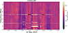 |
Figure 3 LOFAR CS002LBA dynamic spectra for observation L2040075, covering the period of May 10th from 21:35 until 23:35 UTC. The astronomical source of the signal is 3C380. |
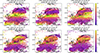 |
Figure 4 Selected vTEC maps in the European sector for the period of May 10th from 21:35 until 23:15 UTC. The resolution is 1° in latitude and 1° in longitude. The green dots represent the position of the IPPs of LOFAR remote and international stations projected to an altitude of 350 km. Units are in TECu. |
The auroral nature of this disturbance is further confirmed by ionosonde observations from Juliusruh (top panels), Chilton (middle panels), and Dourbes (bottom panels) in Figure 5.
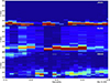 |
Figure 5 Total echo power summed across all ionospheric echoes from the Juliusruh (top), Chilton (middle), and Dourbes (bottom) ionosondes between 21:35 UTC and 23:35 UTC on May 10th, 2024. The plots were generated in arbitrary decibel units. Interpretation should be considered only qualitatively. |
Figure 5 shows a clear decrease in total echo power at Juliusruh, indicative of either attenuated echoes or a reduced number of echoes at 22:13, 22:18, 22:38, 22:43, and 22:48 UTC. Examining the ionograms (not shown), these decreases in total echo power are associated with an increase in the lowest frequency for which there is a return from the ionosphere (fmin) and a reduction in echo power. These periods of elevated fmin and reduced echo power correspond well with the decreases in LOFAR amplitude seen at the German stations (Supplementary material B), suggesting that those decreases in power were likely the result of enhanced medium and high energy particle precipitation, rather than scattering. At Chilton, we similarly see increased fmin at 22:10 UTC and 22:20 UTC (reduced total power after 23:10 UTC is due to there being fewer E-Region echoes rather than attenuation), and at Dourbes, we see increased fmin at 22:20, 22:25, and 22:35 UTC, which also correspond with the observed decreases in source power detected by LOFAR.
This type of absorption observed in LOFAR source data is typically associated with flaring activity. However, it is reported here to result from intense structuring of lower ionospheric layers due to the superstorm.
To further corroborate that ionospheric irregularities sensed by LOFAR during the considered time interval are due to the equatorward displacement of the auroral oval, we analysed the disturbed field.
Figure 6 shows the disturbed magnetic field reconstructed by the magnetometers in a latitudinal range from 40° to 70° N for the entire duration of the LOFAR observation. The solid black line represents the equatorward boundary of the auroral oval, while the two white dashed lines represent the minimum and maximum latitude reached by the LOFAR IPPs projected at an altitude of 120 km, similar to what is reported in Figure 5. By further inspecting the available data from networks of SuperDARN radars (not shown) produced at a temporal resolution of 2 min, it is fully demonstrated that the equatorward expansion of the auroral boundary throughout the storm interval is consistent with the solid black line illustrated within Figure 6.
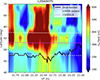 |
Figure 6 Disturbance field measured by the magnetometers as a function of time and latitude. The solid black line represents the equatorward position of the auroral oval, while the two white dashed lines represent the minimum and maximum latitude reached by the LOFAR IPPs (from FR and SE stations, respectively), while the magenta line represents the position of the CS002 IPPs. All the data are projected at an altitude of 120 km. |
Figure 6 illustrates further that the LOFAR CS002 IPPs, projected at an altitude of 120 km, are located inside the estimated boundary of the auroral oval, thereby supporting our hypothesis that the observed ionospheric disturbances are associated with E-layer irregularities located within the displaced auroral oval.
Taken together, these results – LOFAR fading, GNSS TEC enhancement, ionosonde evidence of auroral plasma, and magnetometer boundary shifts – all converge on a consistent physical interpretation: the LOFAR stations observed direct ionospheric effects from the equatorward expansion of the auroral oval during the peak of the May 10th storm. This multi-instrument validation highlights LOFAR’s value in capturing mesoscale ionospheric responses.
3.2 May 11th 03:40–11:40 UT (LOFAR dataset D – source CASSIOPEIA A)
At the beginning of the superstorm’s recovery phase, LOFAR demonstrated its uniqueness by capturing ionospheric dynamics under conditions in which all other ground-based instruments failed to provide a complete picture. To corroborate this, we first examine the S4 index to assess the overall scintillation activity during the morning of May 11th. Figure 7 presents the S4 index calculated over 180-second intervals for the LOFAR station CS002HBA0, spanning the period from 03:40 to 11:40 UTC on May 11th and across a frequency range of 110–190 MHz. The S4 measured for all the other core and international stations is reported in Supplementary material C.
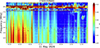 |
Figure 7 LOFAR S4 data from CS002HBA0 for observation L2040001, covering the period of May 11th from 3:40 until 11:40 UTC. The astronomical source of the signal is Cassiopeia A. The plot represents the S4 index, measured at 180s. |
As expected, S4 patterns are very similar across all CSs, with the exception of CS103HBA0, which displays elevated noise levels potentially originating from antenna-specific factors rather than ionospheric effects. The largest S4 values are observed before 06:00 UTC, while scintillation activity is almost absent after 09:00 UTC.
We investigate the concurrent ionospheric conditions using vTEC maps at six distinct time intervals (04:00, 05:00, 06:00, 07:00, 08:00, 09:00 UTC). These maps (Fig. 8a) have a spatial resolution of 1° in latitude and 1° in longitude. In the maps, the green and the red dots represent the IPPs of LOFAR RSs and ISs projected to an altitude of 350 km.
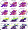 |
Figure 8 vTEC (panel a) and ROTI (panel b) map on the European sector every hour for the period of May 11th from 04:00 until 09:00 UTC. The resolution is 1° in latitude and 1° in longitude. The green dots (Panel a) and the red dots (Panel b) represent the position of the IPPS of LOFAR Remote and International LBA antennas. All the data are projected at an altitude of 350 km. Units are in TECu. |
The vTEC maps in Figure 8a reveal consistently low values (always < 25 TECu) throughout the observational period, particularly evident after 05:00 UTC. ROTI maps (Fig. 8b) highlight the boundaries of the auroral oval; however, the geographical position of the oval depends on the assumed altitude for the projection of the IPPs. All the points of Figure 8 are projected at an altitude of 350 km, which is questionable, as anticipated in the text and demonstrated further. This ambiguity complicates the interpretation of the physical processes responsible for the observed signal disturbances.
To further investigate this phenomenon of reduced TEC and its potential implications for auroral oval identification, we examine ionogram data obtained from the Chilton, Dourbes, and Juliusruh ionosondes recorded from 04:00 UTC to 11:00 UTC on May 11th. The analysis of the ionograms reveals a dominance of absorption features and an absence of discernible traces. These types of absorption features are also apparent within the spectrometers provided by Sodankylä Geophysical Observatory2. During this period, the ionosphere is in G-condition, meaning that the F2 layer has been significantly depleted and is either not present or is present but at a density lower than that of plasma density at peak F1 layer, NmF1. G-conditions make the reconstruction of the ionospheric vertical electron density profile, from the ionosondes data, impossible during the negative phase of the storm and the uplift event, as shown in Supplementary material A.
To investigate the position of the LOFAR IPPs (at 120 km) with respect to the position of the AEB, Figure 9 shows the disturbed magnetic field reconstructed by the magnetometers in a latitudinal range from 40° to 70° N for the entire duration of the LOFAR observation. The solid black line represents the position of the equator-ward position of the auroral oval, while the two white dashed lines represent the minimum and maximum latitude reached by the LOFAR antennas – French (FR) and Swedish (SE) stations respectively-, while the magenta line represents the position of the CS002. In this case, the magenta line lies closer to the equatorward boundary of the auroral oval than it did on the night of May 10th, even extending below it at times.
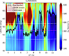 |
Figure 9 Disturbance field measured by the magnetometers as a function of time and latitude. The solid black line represents the equatorward position of the auroral oval, while the two white dashed lines represent the minimum and maximum latitude reached by the LOFAR IPPs (from FR and SE stations, respectively), while the magenta line represents the position of the CS002 IPPs. All the data are projected at an altitude of 120 km. |
Bearing in mind the limitations in assuming 120 km as the height of the IPPs, this configuration is associated with a weaker spectral disturbance, thereby enabling more reliable measurements of the velocity of sub-auroral structures, highlighted in the paper by Themens et al. (2024). Then, before proceeding with the velocity estimates with the methods reported in Sections 2.1.2 and 2.1.3, we checked the robustness and reliability of the Fresnel algorithm against IDOLS observations, and details of such a consistency check are provided in Supplementary material D.
Figure 10 reports the velocities estimated by the two independent methods applied to the data at 140 MHz.
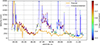 |
Figure 10 Velocity estimates during the storm by using cross-correlation and velocity from Fresnel Frequency identification. The orange line represents the mean velocity of all the core stations obtained using Fresnel algorithm, while the blue line represents the velocity obtained by the cross-correlation algorithm. The colour of the dots of the cross-correlation velocity represents the mean cross-correlation of every baseline at every time interval. Both algorithms refer to LOFAR intensity data at 140 MHz projected at an altitude of 350 km. |
The orange line represents the mean velocity of all the CSs obtained using the Fresnel algorithm, while the blue line represents the velocity obtained by the cross-correlation algorithm. The colour of the dots of the cross-correlation velocity represents the mean cross-correlation of every baseline at every time interval. To exemplify the comparison between the methods, both project the IPPs at an altitude of 350 km, and the cross-correlation velocity has been projected in the same plane observed by the Fresnel algorithm, the plane perpendicular to the line of sight of the core stations’ antennas.
When considering 350 km altitude for the ionospheric layer producing scintillations, both algorithms yield velocities of a similar order of magnitude (hundreds of m/s); however, discrepancies in the numerical values are evident, particularly during the interval from 06:00 to 09:30 UTC. After 9:30 UTC, the mean cross-correlation starts lowering, which also corresponds to the period when the frozen-in assumption begins to fade, as checked by means of the method reported in Grzesiak et al. (2022) (not shown).
3.2.1 Effective altitude evaluation and comparison with ionosonde measurements
Following the method described in Section 2.1.4, we estimate an effective altitude of the irregularity layer. This is based on using the latter as a free parameter in both velocity estimates at each timestamp, and by imposing that the two methods return the same velocity. The reader is reminded that, in principle, the Fresnel-based velocity can be retrieved with any instrument that has single-frequency capability roughly in the HF to L-band range and records signals with a Nyquist frequency meaningfully exceeding the Fresnel frequency for a specific wavelength and observation geometry. In contrast, the cross-correlation-based velocity is specific to the LOFAR CSs configuration, which enables the unique determination of the effective ionospheric altitude.
In Figure 11a, the green line represents the effective altitude reconstructed by the comparison of the cross-correlation and Fresnel algorithms for the velocity reconstruction. The colour of the scatter plots represents the relative percentage error between the two velocity methods at the found effective altitude. S4 values, measured at the same frequency of 140 MHz, are also shown as a red line. The yellow line represents the hmF2 reconstructed by the Dourbes ionosonde, used as a reference. Data stopped around 4:35 UTC. After this time, the ionosondes were not able to reconstruct the altitude. However, the result shows, even for just a short period of time, a reasonable match.
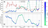 |
Figure 11 In panel a), the green line represents the effective altitude reconstructed by the comparison of the cross-correlation and Fresnel algorithms for the velocity reconstruction. The color of the scatter plots represents the relative percentage error between the two velocity methods. The comparison is done with the velocities measured using the 140 MHz data, as reported in the plot title. S4 values, measured at the same frequency, are also shown as a red line. Panel b) shows the velocity obtained by the cross-correlation method, measured at the effective altitude. The color of the scatter plots represents the relative percentage error between the two velocity methods. |
The comparison algorithm can reconstruct a velocity for the entire duration of the observation. The altitude remains around 500 km until 6:00 UTC in the morning.
Then there is a sudden jump of over 1000 km. Around 8:30 UTC, the altitude starts to rise and reaches 3000 km. This corresponds, however, to a region with a low S4 (<0.03). This decreases the reliability of both the cross-correlation and Fresnel algorithms and so the accuracy of the reconstructed altitude. It is indeed hard to believe that the ionosphere could have reached such a huge height, reminding us how the meaning of the effective altitude must be carefully interpreted.
Indeed, it is important to distinguish the error metric shown in Figure 11 from the absolute effective altitude uncertainty. The plotted error represents the relative consistency between the two velocity retrieval algorithms. While the algorithms mathematically converge with a difference of only ~3% at 09:00 UTC, the physical reliability of the estimate is constrained by the signal conditions.
Specifically, this peak altitude corresponds to a period where the S4 index drops below 0.03 (weak scattering regime). Under such conditions, the determination of the Fresnel frequency becomes increasingly sensitive to noise in the power spectral density, which can lead to systematic artifacts in the altitude retrieval. Consequently, the spike to 3000 km likely represents a breakdown of the method’s sensitivity or the thin-screen assumption rather than a physical plasma uplift to magnetospheric heights. For this reason, we consider the sustained uplift to ~1500 km observed prior to this drop in S4 as the only reliable measurement of the maximum ionospheric vertical displacement.
The strong uplift in the European sector stands out as one of the Mother’s Day superstorm’s most striking phenomena. While traditional instruments experienced a blackout during this specific event, LOFAR was able to continue operating, making it the primary instrument currently providing an estimate of this uplift’s actual magnitude.
The upward displacement resulted mostly from increased Joule heating, which caused the thermosphere to expand rapidly. The heating in an expanded oval drives powerful storm-time thermospheric winds that blow equatorward. This created disturbed neutral composition changes and the large-scale plasma transport, which produced the dramatic uplift (Pierrard et al., 2025).
Figure 11b shows the velocity obtained by the cross-correlation method at the effective altitude, with scatter plot colours representing the relative percentage error between the two velocity methods. At the maximum vertical displacement, the velocity was observed to ramp up to more than 800 m/s. This fast, mostly westward plasma flow is consistent with phenomena such as Polarization Jets/Sub-Auroral Ion Drifts, similar to those reported in the American sector by Themens et al. (2024) and in Eastern Europe by Chernyshov et al. (2025). These phenomena are here detected by LOFAR as km-scale irregularities occurring below the AEB. This differentiates from the small-to-medium scale irregularities detected by the scintillation receivers in the Scandinavian sector within the auroral oval, reported partly in Themens et al. (2024), and further investigated by checking the scintillation data from receivers in Finland managed by the Finnish Meteorological Institute and available in the electronic Space Weather upper atmosphere3, managed by Istituto Nazionale di Geofisica e Vulcanologia (not shown).
Furthermore, the increased westward flow is also consistent with the very low (down to about −1500 nT) values of the IU index (Fig. 2b) that characterised the first half of May 11th. This indicates that strong electric fields in the inner magnetosphere map down to the subauroral region and drive the extremely fast plasma drift.
These LOFAR measurements provide a simultaneous observation of a deeply upward-displaced and fast-moving ionosphere following the superstorm.
The retrieval of the effective altitude also provides a clearer picture of the geographical location of the irregularity layer, which is imprecise in TEC-based and other representations that assume a fixed altitude for the IPPs. Specifically, Figure 12 illustrates the IPPs of LOFAR station CS002HBA0. These IPPs are projected onto both the effective altitude of the ionospheric irregularities (yellow-red markers) derived through our methodology and a fixed altitude of 350 km (blue markers).
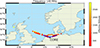 |
Figure 12 Position of LOFAR CS002HBA0 IPPs (yellow-red dots) projected at the effective altitude and at an altitude of 350 km (blue dots). The black X represents the position of the LOFAR core stations. |
Notably, a discernible spatial displacement is observed between the IPP locations determined using the inferred effective altitude and those predicated on the conventional 350 km assumption. This discrepancy underscores the utility of our approach in refining the localization of ionospheric irregularities perturbing LOFAR observations. The retrieved effective altitude is particularly valuable in conditions where ionosonde data are unavailable or inconclusive and constitutes a peculiar measurement, possible only because of the joint use of the two methods on LOFAR data.
3.3 Implications for radio astronomy
Astronomical radio observations at the lowest frequencies (below 20 MHz) have gained interest for many reasons. Science at these frequencies includes direct radio detection of Jupiter-like exoplanets, stellar flare studies, and extragalactic science studying steep-spectrum radio sources like fossil radio plasma from radio galaxies. In normal conditions, the lowest frequencies are not available for ground-based observatories due to the ionospheric cut-off. Also, the lowest frequency observations are often problematic due to ionospheric distortions and radio frequency interference that is reflected from the ionosphere (Chiang et al., 2020).
Between 09:00 UTC and 16:00 UTC on 12th May 2024, the IDOLS observation of Cassiopeia A, made using the CS032, operating between 10 and 80 MHz, did not show significant structuring due to ionospheric effects, based upon the S4 index (Fig. 13). Therefore, at this time, the ionospheric conditions were likely to have been particularly good for very low frequency radio observations. As these conditions occurred some time after the main phase of the geomagnetic storm, it may be possible to use high levels of geomagnetic activity as a precursor for such conditions and to schedule LOFAR observations accordingly.
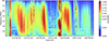 |
Figure 13 LOFAR data for IDOLS observation, covering the period from May 10th at 13:30 UTC until May 14th at 08:30 UTC. The astronomical source of the signal is Cassiopeia A. The plot represents the S4 index, measured at 180s, of the CS0032LBA. |
4 Conclusions
In this investigation, we harnessed the unique capabilities of the LOFAR radio telescope to directly probe the structure and dynamics of the ionosphere during the most extreme space weather conditions of the last two decades.
During the main phase of the superstorm, LOFAR LBA observations of the 3C380 source revealed significant signal fading, coinciding with the equatorward displacement of the auroral oval and related occurrence of E-layer irregularities due to particle precipitation.
Furthermore, the favourable post-storm ionospheric conditions on May 12th, 2024, enable high-quality LOFAR observations of the redshifted H-alpha spectral line, suggesting geomagnetic activity may serve as a precursor for planning such observations.
In addition to ionospheric disturbances, LOFAR also captured a class X 3.9 solar flare and an associated solar radio burst on the morning of May 10th (Supplementary material E), demonstrating its capability to observe both solar and ionospheric phenomena during extreme space weather events.
However, it is during the early hours of the recovery phase on May 11th that LOFAR revealed its uniqueness as an ionospheric probing instrument.
Indeed, LOFAR HBA observations from Cassiopeia A between 04:00 UT and 11:00 UT allowed us to reconstruct fast-moving ionospheric irregularities, for which we estimated drift velocities reaching up to ~800 m/s, associated with a strong upward displacement of the ionosphere, whose effective altitude reached up to 1500 km. LOFAR enabled this first and peculiar determination thanks to the application of two independent techniques – one based on cross-correlation and the other on Fresnel frequency analysis. Indeed, an ionospheric uplift, the lower boundary of which has been found to be up to 1000 km in various sectors, has been reported in the literature, based on ionosonde data (see, e.g. Spogli et al., 2024; Fagundes et al., 2025; Paul et al., 2025). However, we derived the effective, time-resolved estimate of the ionospheric altitude. This approach is particularly valuable in conditions where ionosonde data are unavailable or inconclusive, or when fixing the altitude of IPPs may lead to misleading interpretations. The identified fast plasma flow has been ascribed to Polarization Jets/Sub-Auroral Ion Drifts drifting mostly westward and coinciding with long-lasting conditions of strong westward auroral electrojet activity (IU index down to −1500 nT). The upward displacement resulted mostly from increased Joule heating, which caused the thermosphere to expand rapidly. The heating in an expanded oval drives powerful storm-time thermospheric winds that blow equatorward. This created disturbed composition changes and the large-scale plasma transport, which produced the dramatic uplift observed over Europe.
These results demonstrate the unique capability of LOFAR to provide precious ionospheric information under extreme space weather conditions, offering complementary insights where conventional ground-based instruments may provide a limited picture.
Acknowledgments
We would like to acknowledge the LOFAR Ionospheric Research Group (LIRG) for valuable discussions, collaboration, and support that contributed to this research.
R.B. and L.S. are grateful to Michael Pezzopane (INGV) for the insightful discussion and help with ionosonde data
This paper is based (in part) on results obtained with LOFAR-ERIC equipment. LOFAR (van Haarlem et al., 2013) is the Low Frequency Array designed and constructed by ASTRON. The editor thanks two anonymous reviewers for their assistance in evaluating this paper.
Funding
This work was funded by the Horizon 2020 Programme of the European Commission under Grant Agreement 101007599, project PITHIA-NRF.
P.F., K.K., and A.K. acknowledge the Ministry of Science and Higher Education of Poland for granting funds for the Polish contribution to the LOFAR ERIC, LOFAR2.0 upgrade (decision number: 2021/WK/2) and for maintenance of the LOFAR PL-612 Bałdy station (decision number: 28/530020/SPUB/SP/2022) and Lamkowko Satellite Observatory (decision number: 22/566625/SPUB/SP/2023).
The work at the University of Bath was supported by the UK Natural Environment Research Council (NERC) [grant numbers NE/R009082/1, NE/V002597/1, NE/W003074/1].
L.S., L.A., and C.C. acknowledge the Space It Up project funded by the Italian Space Agency, ASI, and the Ministry of University and Research, MUR, under contract n. 2024-5-E.0- CUP n. I53D24000060005
D.R.T. acknowledges the support of the UK Met Office’s ARCTIC programme and UK NERC FINESSE (NE/W003147/1) and DRIIVE (NE/W003368/1) grants.
A.W., G.D., and B.B. acknowledge the support of the Leverhulme Trust under Research Project Grant RPG-2020-140.
K.B. acknowledges the support of the Office of Naval Research (ONR grant N000142312161)
This publication is part of the project LOFAR Data Valorization (LDV) [project numbers 2020.031, 2022.033, and 2024.047] of the research programme Computing Time on National Computer Facilities using SPIDER that is (co-)funded by the Dutch Research Council (NWO), hosted by SURF through the call for proposals of Computing Time on National Computer Facilities.
Conflicts of Interest
The authors declare no conflicts of interest.
Data availability statement
The k-index data for the Dourbes observatory are provided by the Royal Meteorological Institute (http://ionosphere.meteo.be/geomagnetism/ground_K_dourbes/)
The FMI-IMAGE electrojet indicators and magnetometers data are available at https://space.fmi.fi/image/www/index.php.
GNSS data were obtained from the Madrigal Database, which aggregates data from a global network of GNSS receivers. The data used in this study were accessed via: https://cedar.openmadrigal.org.
Ionosondes data are provided by: https://giro.uml.edu/didbase/.
Magnetometers data are available at: https://supermag.jhuapl.edu/.
The SuperDARN radars data are available at https://superdarn.ca/.
The Sodankylä spectrometers can be observed through https://www.sgo.fi/Data/SpectRiometer/spectrioData.php.
Supplementary material
Supplementary material A
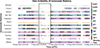 |
Figure A1. Data availability for multiple European ionosonde stations from 9 May to 14 May 2024, with each coloured bar representing a specific ionospheric parameter (e.g., foF2, foF1, etc.) measured at a given station over the set time.The black rectangle highlights the morning of 11 May, when the European ionosonde network experienced an “information blackout”. |
Supplementary material B
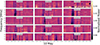 |
Figure B1. LOFAR data for observation L2040075, covering the period of May 10th from 21:35 until 23:35 UTC. The astronomical source of the signal is 3C380. The plot represents the normalised dynamic spectra of the CS002, RS106 and International LBA stations. |
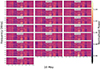 |
Figure B2. LOFAR dynamic spectra for observation L2040075, covering the period of May 10th from 21:35 until 23:35 UTC. The astronomical source of the signal is 3C380. The plot represents the data of the Core LBA stations. |
Supplementary material C
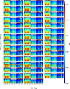 |
Figure C1. LOFAR data for observation L2040001, covering the period of May 11th from 3:40 until 11:40 UTC. The astronomical source of the signal is Cassiopeia A. The plot represents the S4 indexes, measured at 180s, of all the HBA Core antennas. |
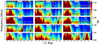 |
Figure C2. LOFAR data for observation L2040001, covering the period of May 11th from 3:40 until 11:40 UTC. The astronomical source of the signal is Cassiopeia A. The plot represents the S4 indexes, measured at 180s, of the CS002, RS106 and International HBA0 antennas. |
Supplementary material D
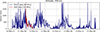 |
Figure D1. Velocity measured using Fresnel algorithm for IDOLS data (blue line) at 60 MHz and for L2040001 observation (red line) at 140 MHz. |
Supplementary material E
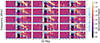 |
Figure E1. LOFAR normalized intensity data for observation L2040063, covering the period of May 10th from 05:58 until 07:58 UTC. The blue line represents the X-ray flux from GOES. |
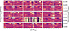 |
Figure E2. LOFAR normalized intensity data for observation L2040071, covering the period of May 10th from 11:25 until 13:25 UTC. Around 12:30 UTC the all the data show a rapid increment at the same instants. This represents the arrival of a solar radio burst. |
References
- Alken, P, Thébault E, Beggan CD, Amit H, Aubert J, et al. 2021. International geomagnetic reference field: the thirteenth generation. Earth Planets Space 73: 49. https://doi.org/10.1186/s40623-020-01288-x. [NASA ADS] [CrossRef] [Google Scholar]
- Boyde, B, Wood AG, Dorrian GD, de Gasperin F, Mevius M. 2025. Statistics of travelling ionospheric disturbances observed using the LOFAR radio telescope. J Space Weather Space Clim 14: 21. https://doi.org/10.1051/swsc/2025002. [Google Scholar]
- Boyde, B, Wood A, Dorrian G, Fallows R, Themens D, et al. 2022. Lensing from small-scale travelling ionospheric disturbances observed using LOFAR. J Space Weather Space Clim 12: 34. https://doi.org/10.1051/swsc/2022030. [CrossRef] [EDP Sciences] [Google Scholar]
- Chabanski, S, de Montety F, Lilensten J, Poedts S, Spogli L. 2025. The power of a name: Toward a unified approach to naming space weather events. Perspect Earth Space Scientists 6 (1): e2025CN000285. https://doi.org/10.1029/2025CN000285. [Google Scholar]
- Chernyshov, AA, Klimenko MV, Nosikov IA, Borchevkina OP, Timchenko AV, et al. 2025. Effects in the upper atmosphere and ionosphere in the subauroral region during Victory Day 2024 Geomagnetic Storm (May 10–12, 2024). Adv Space Res 76 (12): 7325–7350. https://doi.org/10.1016/j.asr.2025.02.015. [Google Scholar]
- Chiang, HC, Dyson T, Egan E, Eyono S, Ghazi N, et al. 2020. The array of long baseline antennas for taking radio observations from the sub-antarctic. J Astron Instrum 09 (04): 2050019. https://doi.org/10.1142/S2251171720500191. [Google Scholar]
- Dorrian, G, Fallows R, Wood A, Themens DR, Boyde B, et al. 2023. LOFAR observations of substructure within a traveling ionospheric disturbance at mid-latitude. Space Weather 21: e2022SW003198. https://doi.org/10.1029/2022SW003198. [CrossRef] [Google Scholar]
- Elvidge, S, Themens DR. 2025. The probability of the May 2024 geomagnetic superstorm. Space Weather 23 (1): e2024SW004113. https://doi.org/10.1029/2024SW004113. [Google Scholar]
- Fagundes, P, Pillat V, Habarulema J, Muella M, Venkatesh K, et al. 2025. Equatorial ionization anomaly disturbances (EIA) triggered by the May 2024 solar Coronal Mass Ejection (CME): The strongest geomagnetic superstorm in the last two decades. Adv Space Res 76 (12): 7375–7389. https://doi.org/10.1016/j.asr.2025.02.007. [Google Scholar]
- Fallows, RA, Forte B, Astin I, Allbrook T, Arnold A, et al. 2020. A LOFAR observation of ionospheric scintillation from two simultaneous travelling ionospheric disturbances. J Space Weather Space Clim 10: 10. https://doi.org/10.1051/swsc/2020010. [CrossRef] [EDP Sciences] [Google Scholar]
- Flisek, P, Forte B, Fallows R, Kotulak K, Krankowski A, et al. 2023. Towards the possibility to combine LOFAR and GNSS measurements to sense ionospheric irregularities. J Space Weather Space Clim 13: 27. https://doi.org/10.1051/swsc/2023021. [Google Scholar]
- Forte, B, Radicella SM. 2002. Problems in data treatment for ionospheric scintillation measurements. Radio Sci 37 (6): 1096. https://doi.org/10.1029/2001RS002508. [Google Scholar]
- Forte, B, RA Fallows, Bisi MM, Zhang J, Krankowski A, et al. 2022. Interpretation of radio wave scintillation observed through LOFAR radio telescopes. Astrophys J Suppl Ser 263 (2): 36. https://doi.org/10.3847/1538-4365/ac6deb. [CrossRef] [Google Scholar]
- Foster, JC, Erickson PJ, Nishimura Y, Zhang SR, Bush DC, et al. 2024.Imaging the May 2024 extreme aurora with ionospheric total electron content. Geophys Res Lett 51 (20): e2024GL111981. https://doi.org/10.1029/2024GL111981. [Google Scholar]
- Fremouw, EJ, Leadabrand RL, Livingston RC, Cousins MD, Rino CL, et al. 1978. Early results from the DNA Wideband satellite experiment–Complex-signal scintillation. Radio Sci 13 (1): 167–187. https://doi.org/10.1029/RS013i001p00167. [CrossRef] [Google Scholar]
- Ghidoni, R, Spogli L, Mevius M, Cesaroni C, Alfonsi L, Beser K, et al. 2024. Ionospheric response to the January 2022 geomagnetic storm using LOFAR and GNSS. J Space Weather Space Clim 15: 18. https://doi.org/10.1051/swsc/2025052. [Google Scholar]
- Gjerloev, JW. 2012. The SuperMAG data processing technique. J Geophys Res 117: A09213. https://doi.org/10.1029/2012JA017683. [Google Scholar]
- Grzesiak, M, Pożoga M, Matyjasiak B, Przepiórka D, Beser K, et al. 2022. Determining ionospheric drift and anisotropy of irregularities from LOFAR core measurements: Testing hypotheses behind estimation. Remote Sens 14 (18): 4655. https://doi.org/10.3390/rs14184655. [Google Scholar]
- Huang, X, Reinisch BW. 1996. Vertical electron density profiles from digisonde ionograms. The average representative profile. Ann Geophys 39(4). https://doi.org/10.4401/ag-4010. [Google Scholar]
- Ippolito, A, Alberti T, Giannattasio F. 2025. Modeling the magnetic connection from earth to solar corona during the May 11 geomagnetic superstorm. Astrophys J 979 (2): 146. https://doi.org/10.3847/1538-4357/ada35a. [Google Scholar]
- Jin, Y, Kotova D, Clausen LBN, Miloch WJ. 2025. Significant plasma density depletion from high- to mid-latitude ionosphere during the Super Storm in May 2024. Geophys Res Lett 52(5): e2024GL113997. https://doi.org/10.1029/2024GL113997. [Google Scholar]
- Johnsen, MG. 2013. Real-time determination and monitoring of the auroral electrojet boundaries. J Space Weather Space Clim 3: A28. https://doi.org/10.1051/swsc/2013050. [Google Scholar]
- Kataoka, R, Reddy SA, Nakano S, Pettit J, Nakamura Y. 2024. Extended magenta aurora as revealed by citizen science. Sci Rep 14: 25849. https://doi.org/10.1038/s41598-024-75184-9. [Google Scholar]
- Mevius, M, van der Tol S, Pandey V, Vedantham H, Brentjens M, et al. 2016. Probing ionospheric structures using the LOFAR radio telescope. Radio Sci 51(7):927–941. https://doi.org/10.1002/2016RS006028. [CrossRef] [Google Scholar]
- Paul, KS, Moses M, Haralambous H, Oikonomou C. 2025. Effects of the Mother’s Day superstorm (10–11 May 2024) over the global ionosphere. Remote Sens 17 (5): 859. https://doi.org/10.3390/rs17050859. [Google Scholar]
- Pi, X, Mannucci AJ, Lindqwister UJ, Ho CM. 1997. Monitoring of global ionospheric irregularities using the worldwide GPS network. Geophys Res Lett 24 (18): 2283–2286. https://doi.org/10.1029/97GL02273. [CrossRef] [Google Scholar]
- Pierrard, V, Verhulst TG, Chevalier JM, Bergeot N, Winant A. 2025.Effects of the geomagnetic superstorms of 10–11 May 2024 and 7–11 October 2024 on the ionosphere and plasmasphere. Atmosphere 16 (3): 299. https://doi.org/10.3390/atmos16030299. [Google Scholar]
- Ranjan, AK, Nailwal D, Sunil Krishna MV, Kumar A, Sarkhel S. 2024. Evidence of potential thermospheric overcooling during the May 2024 geomagnetic superstorm. J Geophys Res: Space Phys 129 (12): e2024JA033148. https://doi.org/10.1029/2024JA033148. [Google Scholar]
- Rideout, W, Coster A. 2006. Automated GPS processing for global total electron content data. GPS Solu 10: 219–228. https://doi.org/10.1007/s10291-006-0029-5. [CrossRef] [Google Scholar]
- Romano, P, Elmhamdi A, Marassi A, Contarino L. 2024. Analyzing the sequence of phases leading to the formation of the active region 13664, with potential Carrington-like characteristics. Astrophys J Lett 973 (1): L31. https://doi.org/10.3847/2041-8213/ad77cb. [Google Scholar]
- Savitzky, A, Golay MJE. 1964. Smoothing and differentiation of data by simplified least squares procedures. Anal Chem 36 (8): 1627–1639. https://doi.org/10.1021/ac60214a047. [Google Scholar]
- Spogli, L, Alberti T, Bagiacchi P, Cafarella L, Cesaroni C, et al. 2024. The effects of the May 2024 Mother’s Day superstorm over the mediterranean sector: from data to public communication. Ann Geophys 67 (2): PA218. https://doi.org/10.4401/ag-9117. [Google Scholar]
- Spogli, L, Ghobadi H, Cicone A, Alfonsi L, Cesaroni C, et al. 2021. Adaptive phase detrending for GNSS scintillation detection: A case study over antarctica. IEEE Geosci Remote Sens Lett 19: 1–5. https://doi.org/10.1109/LGRS.2021.3067727. [Google Scholar]
- Tanskanen, EI. 2009. A comprehensive high‐throughput analysis of substorms observed by IMAGE magnetometer network: Years 1993–2003 examined. J Geophys Res: Space Phys 114 (A5): A05204. https://doi.org/10.1029/2008JA013682. [Google Scholar]
- Taylor, GI, Lond A. 1935. Statistical theory of turbulence. Proc R Soc 151 (873): 421–444. https://doi.org/10.1098/rspa.1935.0158. [Google Scholar]
- Teunissen, P, Montenbruck O. 2017. Springer handbook of global navigation satellite systems. Springer International. https://doi.org/10.1007/978-3-319-42928-1. [Google Scholar]
- Themens, DR, Elvidge S, McCaffrey A, Jayachandran PT, Coster A, et al. 2024. The high latitude ionospheric response to the major May 2024 geomagnetic storm: A synoptic view. Geophys Res Lett 51: e2. https://doi.org/10.1029/2024GL111677. [Google Scholar]
- Themens, DR, Reid B, Elvidge S. 2022. ARTIST ionogram autoscaling confidence scores: Best practices. URSI Radio Sci Lett 4: 1–5. https://doi.org/10.46620/22-0001. [Google Scholar]
- Trigg, H, Dorrian GD, Boyde B, Wood AG, Fallows RA, et al. 2024. Observations of high definition symmetric quasi-periodic oscillations in the mid-latitude ionosphere with LOFAR. J Geophys Res Space Phys 129 (7): 2023JA032336. https://doi.org/10.1029/2023JA032336. [Google Scholar]
- Tulasi Ram, S, Veenadhari B, Dimri AP, Bulusu J, Bagiya M, et al. 2024. Super-intense geomagnetic storm on 10–11 May 2024: Possible mechanisms and impacts. Space Weather 22: e2024SW004126. https://doi.org/10.1029/2024SW004126. [Google Scholar]
- van Haarlem, MP, Wise MW, Gunst AW, Heald G, McKean JP, et al. 2013. LOFAR: The low-frequency array. Astron Astrophys 556: A2. https://doi.org/10.1051/0004-6361/201220873. [Google Scholar]
- Vierinen, J, Coster AJ, Rideout WC, Erickson PJ, Norberg J. 2016. Statistical framework for estimating GNSS bias. Atmos Meas Tech 9: 1303–1312. https://doi.org/10.5194/amt-9-1303-2016. [Google Scholar]
- Wei, Y, Zhao B, Li G, Wan W. 2015. Electric field penetration into Earth’s ionosphere: A brief review for 2000–2013. Sci Bull 60 (8): 748–761. https://doi.org/10.1007/s11434-015-0749-4. [Google Scholar]
- Wernik, AW, Alfonsi L, Materassi M. 2007. Scintillation modeling using in situ data. Radio Sci 42: RS1002. https://www.doi.org/10.1029/2006RS003512. [Google Scholar]
- Wood, A, Dorrian G, Boyde B, Fallows R, Themens D, et al.. 2024. Quasi-stationary substructure within a sporadic E layer observed by the Low-Frequency Array (LOFAR). J Space Weather Space Clim 14: 27. https://doi.org/10.1051/swsc/2024024. [CrossRef] [EDP Sciences] [Google Scholar]
- Yeh, KC, Liu CH. 1982. Radio wave scintillations in the ionosphere. Proc IEEE 70 (4): 324–360. https://doi.org/10.1109/PROC.1982.12313. [CrossRef] [Google Scholar]
Cite this article as: Ghidoni R, Spogli L, Dorrian G, Mevius M, Flisek P, et al. 2026. LOFAR uniqueness under extreme ionospheric conditions: The May 2024 Mother’s Day superstorm. J. Space Weather Space Clim. 16, 6. https://doi.org/10.1051/swsc/2025059.
All Tables
Details of the LOFAR observations employed in the analysis. The table provides the associated letter code for each observation, as reported in Figure 2, the LOFAR observation ID, the observed celestial radio source, the antenna type used (LBA or HBA), and the start and end times (UTC) for each observation period.
All Figures
|
Figure 1 Location of LOFAR antennas. Panel a) shows the position of International stations (red dots), IMAGE magnetometers (blue dots), and Ionosondes (green dots). Panel b) shows the position of Remote stations, and panel c) shows the position of Core stations. |
| In the text | |
|
Figure 2 Panel a) shows the K-index from Dourbes from 15:00 UT on May 9th until 02:00 UT on May 14th. The color of the bars indicates the NOAA Space Weather Scale for geomagnetic storms4. Panel b) shows the electrojet indicators IE, IL, and IU for IMAGE magnetometers. The grey bars represent the five all-stations LOFAR observations, while the blue one represent the period of available IDOLS data. |
| In the text | |
|
Figure 3 LOFAR CS002LBA dynamic spectra for observation L2040075, covering the period of May 10th from 21:35 until 23:35 UTC. The astronomical source of the signal is 3C380. |
| In the text | |
|
Figure 4 Selected vTEC maps in the European sector for the period of May 10th from 21:35 until 23:15 UTC. The resolution is 1° in latitude and 1° in longitude. The green dots represent the position of the IPPs of LOFAR remote and international stations projected to an altitude of 350 km. Units are in TECu. |
| In the text | |
|
Figure 5 Total echo power summed across all ionospheric echoes from the Juliusruh (top), Chilton (middle), and Dourbes (bottom) ionosondes between 21:35 UTC and 23:35 UTC on May 10th, 2024. The plots were generated in arbitrary decibel units. Interpretation should be considered only qualitatively. |
| In the text | |
|
Figure 6 Disturbance field measured by the magnetometers as a function of time and latitude. The solid black line represents the equatorward position of the auroral oval, while the two white dashed lines represent the minimum and maximum latitude reached by the LOFAR IPPs (from FR and SE stations, respectively), while the magenta line represents the position of the CS002 IPPs. All the data are projected at an altitude of 120 km. |
| In the text | |
|
Figure 7 LOFAR S4 data from CS002HBA0 for observation L2040001, covering the period of May 11th from 3:40 until 11:40 UTC. The astronomical source of the signal is Cassiopeia A. The plot represents the S4 index, measured at 180s. |
| In the text | |
|
Figure 8 vTEC (panel a) and ROTI (panel b) map on the European sector every hour for the period of May 11th from 04:00 until 09:00 UTC. The resolution is 1° in latitude and 1° in longitude. The green dots (Panel a) and the red dots (Panel b) represent the position of the IPPS of LOFAR Remote and International LBA antennas. All the data are projected at an altitude of 350 km. Units are in TECu. |
| In the text | |
|
Figure 9 Disturbance field measured by the magnetometers as a function of time and latitude. The solid black line represents the equatorward position of the auroral oval, while the two white dashed lines represent the minimum and maximum latitude reached by the LOFAR IPPs (from FR and SE stations, respectively), while the magenta line represents the position of the CS002 IPPs. All the data are projected at an altitude of 120 km. |
| In the text | |
|
Figure 10 Velocity estimates during the storm by using cross-correlation and velocity from Fresnel Frequency identification. The orange line represents the mean velocity of all the core stations obtained using Fresnel algorithm, while the blue line represents the velocity obtained by the cross-correlation algorithm. The colour of the dots of the cross-correlation velocity represents the mean cross-correlation of every baseline at every time interval. Both algorithms refer to LOFAR intensity data at 140 MHz projected at an altitude of 350 km. |
| In the text | |
|
Figure 11 In panel a), the green line represents the effective altitude reconstructed by the comparison of the cross-correlation and Fresnel algorithms for the velocity reconstruction. The color of the scatter plots represents the relative percentage error between the two velocity methods. The comparison is done with the velocities measured using the 140 MHz data, as reported in the plot title. S4 values, measured at the same frequency, are also shown as a red line. Panel b) shows the velocity obtained by the cross-correlation method, measured at the effective altitude. The color of the scatter plots represents the relative percentage error between the two velocity methods. |
| In the text | |
|
Figure 12 Position of LOFAR CS002HBA0 IPPs (yellow-red dots) projected at the effective altitude and at an altitude of 350 km (blue dots). The black X represents the position of the LOFAR core stations. |
| In the text | |
|
Figure 13 LOFAR data for IDOLS observation, covering the period from May 10th at 13:30 UTC until May 14th at 08:30 UTC. The astronomical source of the signal is Cassiopeia A. The plot represents the S4 index, measured at 180s, of the CS0032LBA. |
| In the text | |
|
Figure A1. Data availability for multiple European ionosonde stations from 9 May to 14 May 2024, with each coloured bar representing a specific ionospheric parameter (e.g., foF2, foF1, etc.) measured at a given station over the set time.The black rectangle highlights the morning of 11 May, when the European ionosonde network experienced an “information blackout”. |
| In the text | |
|
Figure B1. LOFAR data for observation L2040075, covering the period of May 10th from 21:35 until 23:35 UTC. The astronomical source of the signal is 3C380. The plot represents the normalised dynamic spectra of the CS002, RS106 and International LBA stations. |
| In the text | |
|
Figure B2. LOFAR dynamic spectra for observation L2040075, covering the period of May 10th from 21:35 until 23:35 UTC. The astronomical source of the signal is 3C380. The plot represents the data of the Core LBA stations. |
| In the text | |
|
Figure C1. LOFAR data for observation L2040001, covering the period of May 11th from 3:40 until 11:40 UTC. The astronomical source of the signal is Cassiopeia A. The plot represents the S4 indexes, measured at 180s, of all the HBA Core antennas. |
| In the text | |
|
Figure C2. LOFAR data for observation L2040001, covering the period of May 11th from 3:40 until 11:40 UTC. The astronomical source of the signal is Cassiopeia A. The plot represents the S4 indexes, measured at 180s, of the CS002, RS106 and International HBA0 antennas. |
| In the text | |
|
Figure D1. Velocity measured using Fresnel algorithm for IDOLS data (blue line) at 60 MHz and for L2040001 observation (red line) at 140 MHz. |
| In the text | |
|
Figure E1. LOFAR normalized intensity data for observation L2040063, covering the period of May 10th from 05:58 until 07:58 UTC. The blue line represents the X-ray flux from GOES. |
| In the text | |
|
Figure E2. LOFAR normalized intensity data for observation L2040071, covering the period of May 10th from 11:25 until 13:25 UTC. Around 12:30 UTC the all the data show a rapid increment at the same instants. This represents the arrival of a solar radio burst. |
| In the text | |
Current usage metrics show cumulative count of Article Views (full-text article views including HTML views, PDF and ePub downloads, according to the available data) and Abstracts Views on Vision4Press platform.
Data correspond to usage on the plateform after 2015. The current usage metrics is available 48-96 hours after online publication and is updated daily on week days.
Initial download of the metrics may take a while.