| Issue |
J. Space Weather Space Clim.
Volume 16, 2026
Topical Issue - Space Climate: Solar Extremes, Long-Term Variability, and Impacts on Earth’s System
|
|
|---|---|---|
| Article Number | 12 | |
| Number of page(s) | 13 | |
| DOI | https://doi.org/10.1051/swsc/2026010 | |
| Published online | 07 May 2026 | |
Technical Article
Using solar ultraviolet irradiance measurements from GOES/EXIS to nowcast flare X-ray properties
1
University of Johannesburg, Department of Physics, Johannesburg, South Africa
2
South African National Space Agency, Hermanus 7200, South Africa
3
University of the Western Cape, Department of Physics and Astronomy, Robert Sobukwe Road, Bellville 7535, South Africa
4
University of Colorado Boulder, Laboratory for Atmospheric and Space Physics, 1234 Innovation Dr., Boulder CO 80303, USA
* Corresponding author: This email address is being protected from spambots. You need JavaScript enabled to view it.
Received:
23
June
2025
Accepted:
18
March
2026
Abstract
Context. X-rays emitted by solar flares change the properties of the Earth’s ionosphere and can damage to technological systems. Space weather forecasters monitor the X-ray irradiance from the Sun and issue warnings to mitigate these potentially harmful effects. Other wavelengths of solar irradiance are also observed operationally, and might provide advanced information about a flare’s X-ray properties. Aims. We investigate whether extreme ultraviolet (EUV) emissions can provide advance information about the strength and duration of 0.1–0.8 nm soft X-ray (SXR) solar flares. Specifically, we assess the predictive capability of He I (121.6 nm; Lyman-alpha), He II (30.4 nm), and the Mg II index in relation to SXR flare characteristics, with the goal of improving flare nowcasting. Methods. We analyzed operational spectral irradiance measurements from the Extreme Ultraviolet Sensor (EUVS) and the X-ray Sensor (XRS) aboard the Geostationary Operational Environmental Satellite-16 (GOES-16). The dataset includes all M- and X-class flares observed between 2017 and May 2025. We examined correlations between the timing and magnitude of EUV and SXR peaks, including lead times, flare durations, and peak intensities. Results. EUV emissions peak before SXR emissions in approximately 76% of cases. For He II, the average lead time is 4.69 min for X-class flares and 4.09 min for M-class flares. Lyman-alpha leads SXR emissions by approximately 4.98 min for X-class and 4.90 min for M-class flares, while Mg II leads by an average of 5.45 min for X-class and 4.75 min for M-class flares. Conclusions. He II shows the strongest correlation with SXR properties: flare durations correlate at r = 0.63 for M-class and r = 0.72 for X-class flares, while peak strength shows a moderate correlation (r = 0.53). He II enhancements exceeding 20% above the background are strong indicators of X-class flares, with fewer than 1% of M-class flares exhibiting such increases. Lyman-alpha demonstrates moderate predictive value for flare duration (r = 0.49 for M-class and r = 0.63 for X-class) and a weak correlation with flare strength (r = 0.32). The Mg II index similarly correlates moderately with SXR duration (r = 0.48 for M-class and r = 0.67 for X-class) and weakly with flare strength (r = 0.43).
Key words: Solar flares / X-rays / Ultraviolet solar irradiance / GOES-R
© A. Mthethwa & M. Snow Published by EDP Sciences 2026
 This is an Open Access article distributed under the terms of the Creative Commons Attribution License (https://creativecommons.org/licenses/by/4.0), which permits unrestricted use, distribution, and reproduction in any medium, provided the original work is properly cited.
1 Introduction
Solar flares are among the most energetic events in the solar atmosphere, releasing immense energy ranging from 1026 to 1032 erg over periods lasting from minutes to hours (Hudson 2011). These events emit radiation across the electromagnetic spectrum (Gold & Hoyle 1960) and can generate energetic particles capable of rapidly modifying the Earth’s ionosphere-thermosphere (IT) system, thereby affecting technological infrastructure, including high-frequency radio communication, GNSS positioning, satellite operations, communication networks, and power grids. It is primarily the X-ray and extreme ultraviolet (EUV) components of flare radiation that affect the Earth’s ionosphere (Handzo et al. 2014), with the severity of the effect varying based on the flare’s intensity and duration (Guyer & Can 2013). The ionosphere is commonly divided into the D, E, and F regions, each characterized by different neutral composition and ionization mechanisms. The F region, typically the most ionized layer of the ionosphere, is particularly important for high-frequency (HF) radio wave propagation (Fang et al. 2012). The impact of flare radiation on the ionosphere is strongly altitude- and wavelength-dependent. EUV radiation primarily affects the E and F regions (Li et al. 2012; Le et al. 2013), enhancing photoionization and increasing electron densities, while soft X-ray (1–8 Å) emission significantly enhances ionization in the lower E and D regions (Qian et al. 2019). Observational and modeling studies have demonstrated that rapid increases in EUV and SXR flux during flares lead to substantial increases in total electron content (TEC), with enhancements of up to 30% in the subsolar ionosphere within approximately five minutes (Tsurutani et al. 2009; Qian et al. 2011; Bekker et al. 2024; O’Hare et al. 2025). Large flares are often accompanied by Coronal Mass Ejections (CMEs), large clouds of solar plasma that can span hundreds of thousands of kilometers (Gosling et al. 1976; MacQueen & Fisher 1983). Together, flares and CMEs are major drivers of space weather variability, making it essential to understand the physical mechanisms that control their evolution and observable signatures.
The standard model of solar flares, commonly referred to as the CSHKP model (Carmichael 1964; Sturrock 1966; Hirayama 1974; Kopp & Pneuman 1976), provides a framework for understanding how these events unfold. It builds on the empirical relationship known as the Neupert effect (Neupert 1968), which describes a correlation between the SXR flux and the time integral of hard X-ray (HXR) flux. This correlation suggests that the heated plasma and energetic electrons are causally connected: the plasma responsible for the SXR emission is heated primarily by energy deposited by flare-accelerated particles. The relationship implies that magnetic reconnection supplies the energy required for particle acceleration. According to the CSHKP model, the flaring process begins with the gradual buildup of magnetic energy in the corona, driven by convection, the solar dynamo, and the Sun’s differential rotation, which stresses and distorts magnetic field lines until they become susceptible to reconnection (Aschwanden 2004; Jafari & Vishniac 2018). Once reconnection occurs, particles are accelerated along magnetic field lines toward the chromosphere. Upon encountering the dense chromosphere, the particles lose energy primarily through Coulomb collisions, which serve as the dominant mechanism for heating the plasma. Only a small fraction of the particles undergo bremsstrahlung interactions, producing hard X-ray emission (Panos 2021). This energy deposition drives chromospheric evaporation (Milligan & Dennis 2009), whereby heated plasma expands upward and fills the overlying flare loops. Observations confirm that this evaporated hot plasma is the dominant source of coronal SXR and EUV radiation during the flare’s main phase (Neupert 1968; Silva et al. 1997). Although solar flares are initiated by magnetic reconnection in the corona, a substantial fraction of their radiative output originates from energy deposited in the chromosphere (e.g., Hudson 1972). This sequence of energy release, particle transport, plasma heating, and radiative response forms the foundation of understanding flare dynamics.
The complex mechanisms behind solar flares have been the subject of extensive research for decades, aiming to understand their triggers and their impacts on the Sun and heliosphere (e.g., Tandberg-Hanssen & Emslie 1988; Fletcher et al. 2011; Hudson 2011). In recent years, this research has gained renewed urgency due to the need for early-warning systems capable of mitigating the effects of flares on modern technological infrastructure. A key focus has been the analysis of ultraviolet emissions as potential precursors to SXR emission. Statistical analyses have played a major role in categorizing flare behavior. For instance, Jing et al. (2020) examined 658 M- and X-class flares, categorizing them based on the relative timing of Lyman-alpha and SXR peak flux. They found that Type I flares, which accounted for 76.8% of the sample, were the most common. In these flares, Lyman-alpha emission peaks before the SXR emission, a signature often associated with nonthermal heating. Type III flares accounted for 21.7% of the sample, with Lyman-alpha emission peaking later than SXR emission, usually during the gradual phase, and associated with thermal plasma cooling. Type II flares are the least common (1.5%) and exhibit nearly simultaneous peaks in Lyman-alpha and SXR emission, typically within 10 seconds. These results are consistent with observational studies showing that Lyman-alpha emission during flares can be driven by both nonthermal and thermal processes (Li et al. 2022; Greatorex et al. 2023). Milligan et al. (2020) analyzed 477 M- and X-class flares and reported that 95% exhibited Lyman-alpha enhancements of at most 10% above a 24-hour modal fit background, with a maximum enhancement of approximately 30%. Subsequently, Milligan (2021) refined this approach, using a one-hour time range to estimate the background, and analyzed 443 M-class and 31 X-class flares. Their findings revealed that Lyman-alpha enhancements on average range from 1% to 4%. Brekke et al. (1996) reported a 6% enhancement for a single X3 flare observed by UARS/SOLSTICE.
Building on previous investigations of chromospheric flare diagnostics, the present analysis focuses on three EUV spectral lines that provide complementary insights into flare-driven atmospheric dynamics. SXR and EUV emissions originate from different layers of the solar atmosphere. The aim of this work is to determine whether relationships exist between the SXR (0.1–0.8 nm) response and the Lyman-alpha, He II (30.4 nm), and Mg II index variability. The He II line forms at approximately 60,000 K in the lower transition region (Bhatnagar & Livingston 2005). In the solar ultraviolet (UV) spectra, hydrogen Lyman-alpha (H I Lyman-alpha) is the strongest line at 121.6 nm (Curdt et al. 2001). This optically thick line (Vial 1982b; Woods et al. 1995) forms largely in the chromosphere and transition region, with a central reversal in its core. Lyman-alpha irradiance increases significantly during a flare (e.g., Woods et al. 2004; Milligan et al. 2012), and recent studies demonstrate that its temporal and spatial evolution closely tracks that of He II (30.4 nm) (Li et al. 2022), suggesting both lines are shaped by related processes in the lower atmosphere. Similarly, the Mg II index, derived from the core-to-wing ratio of the Mg II h and k lines near (280.0 nm) (Heath & Schlesinger 1986), is a chromospheric proxy valuable for estimating other solar ultraviolet emissions (Cebula et al. 1992). During a flare, this line remains optically thick (Kerr et al. 2015). Because these EUV spectral lines are formed at different temperatures and heights in the solar atmosphere, their intensities respond differently to flare-driven heating, density enhancements, and changes in ionization balance, leading to line-to-line variability during solar flares (Thiemann et al. 2017). However, their high background emission often makes it difficult to detect flare-driven irradiance changes. Among the lines considered, Lyman-alpha exhibits the highest background flux, while enhancements are more pronounced in the other channels due to their comparatively lower baselines. For example, Woods et al. (2000) reported that the average Lyman-alpha variability caused by the 27-day solar rotation during Solar Cycles 18–22 was 5% at solar minimum and 11% at solar maximum. The change in the Mg II index from solar minimum to maximum is approximately 14% of the long-term mean of the smoothed Mg II time series (Snow et al. 2019). If relationships exist between the timing and strength of EUV emissions and the SXR response, they should appear across a representative set of flares. To investigate this, we examine GOES-16 observations of He II (30.4 nm), Lyman-alpha, and the Mg II index, analyzing how their temporal evolution compares with the corresponding SXR emission. For each flare, we identify the onset, peak, and decay phases in both the EUV and SXR light curves, and measure any lead or lag between them. We then compare the durations and peak intensities statistically to determine how different layers of the solar atmosphere respond during energy release. This approach allows us to test whether early EUV enhancements consistently align with the timing of the main SXR peak and whether these patterns differ between M- and X-class flares. This paper is organized as follows. Section 2 describes the instruments and data used in this study. Section 3 outlines the flare selection criteria and data-processing methods. Section 4 presents the statistical results, including timing correlations and flux relationships between the EUV and SXR emissions. Section 5 summarizes our findings and discusses their implications for understanding the coupling between chromospheric and coronal flare signatures.
2 Instrumentation
The SXR and EUV spectral lines we analyzed are measured by the Extreme Ultraviolet and X-Ray Irradiance Sensor (EXIS; Machol et al. 2020) instrument onboard the GOES-R series satellites, primarily GOES-16, located at 75° W in the GOES-East position. GOES-16 was launched on November 19, 2016, and became operational in early 2017 (Goodman et al. 2019). EXIS is located on the Sun Pointing Platform of the satellite and houses two sensors: the Extreme Ultraviolet Sensor (EUVS; Eparvier et al. 2009) and the X-Ray Sensor (XRS; Woods et al. 2024). EXIS provides detailed information on solar variability and flare activity with enhanced technology and flare location capability compared to previous GOES instruments. XRS measures solar spectral irradiance (SSI) in the soft X-ray range through two channels: XRS-A (0.05–0.4 nm) and XRS-B (0.1–0.8 nm). The two XRS channels include silicon diode detectors and are further categorized by size and function (Machol et al. 2021). These include smaller quadrant diodes (XRS-A2 and XRS-B2) and larger diodes (XRS-A1 and XRS-B1). The smaller XRS-A2 and XRS-B2 diodes are quadrant detectors designed to detect higher levels of X-ray flux, which are typical during intense solar flares. The quadrant structure of these diodes also allows for the approximate localization of flares on the solar disk by providing rough spatial information. The larger diodes, XRS-A1 and XRS-B1, are better suited for monitoring lower levels of X-ray flux, capturing data even during quieter solar conditions or the less intense phases of flares. The EUVS measures solar irradiance at specific EUV wavelengths, with a focus on spectral lines that are crucial for understanding the thermosphere heating and ionosphere ionization. EUVS measures seven solar lines and the Mg II core-to-wing ratio (Mg II index; McClintock et al. 2025), covering wavelengths from 25.6 nm to 280.3 nm, with sources ranging from the transition region to the chromosphere. EUVS-A observes and quantifies coronal emissions, spectral lines such as He II at 25.6 nm, Fe XV at 28.4 nm, and He II at 30.4 nm. EUVS-B, on the other hand, captures and analyzes transition region emissions such as C III at 117.5 nm, H I at 121.6 nm (known as Lyman-alpha), C II at 133.5 nm, and the blended Si IV/O IV line at 140.5 nm. Lastly, EUVS-C measures the chromosphere, focusing on the measurement of the Mg II Index (McClintock et al. 2025).The individual EUVS-C measurements from GOES-16 have an uncertainty of 0.01% (McClintock et al. 2025).
3 Data Reduction and Analysis
The data used in this analysis are publicly available through NOAA’s National Centers for Environmental Information1. This study focused on M- and X-class flares. We analyzed 1-minute averages derived from 3-second integrated measurements of EUV and SXR irradiance, expressed in watts per square meter (W m−2). Additionally, we used GOES daily averages and minimum irradiance values to establish baseline levels for identifying flare-related enhancements. These daily averages and minimum values represent unique Level 2 GOES EXIS data products. Our initial dataset consisted of 1460 M-class and 78 X-class solar flares observed between February 2017 and April 2025. To ensure the reliability and accuracy of the dataset used to analyze the temporal evolution and intensity of flare emissions, we applied the following strict selection criteria:
-
(1)
Data availability and quality: Each flare was required to have continuous, high-quality light curves for all investigated spectral lines throughout the analysis period. Only data flagged as good_quality and free from instrumental artifacts, data gaps, or geocoronal effects were included (Machol et al. 2021).
-
(2)
Temporal definition of flare events: To ensure consistency across the sample, only flares with clearly determined start, peak, and end times, as defined by the GOES flare catalog were retained. A well-defined flare event was characterized by a distinct and impulsive rise from a stable pre-flare background in the GOES 0.1–0.8 nm light curve, a well-defined maximum, and a gradual decay towards background levels.
-
(3)
Statistical significance of EUV enhancement: Flares were excluded if the EUV peak intensity did not exceed at least two standard deviations above the pre-flare background. This threshold ensured that only statistically significant EUV responses were analyzed, minimizing the chance of interpreting background noise or minor fluctuations as genuine flare activity.
-
(4)
Temporal classification of EUV and SXR peaks: Each flare was classified according to the relative timing of its EUV and SXR peak emissions, following the procedure of Mthethwa (2024), adapted from Jing et al. (2020). This classification was applied to the Lyman-alpha, He II (30.4 nm), and Mg II index lines. Events were categorized based on whether the EUV peak occurred before, near, or after the SXR peak. The present analysis focuses on Type I events, in which the EUV peak precedes the SXR peak, enabling investigation of chromospheric-coronal timing relationships.
After manually applying these selection criteria, 78 X-class and 1,261 M-class flares satisfied criteria (1)–(3). Of these, 57 X-class and 965 M-class flares (approximately 76%) also satisfied criterion (4) and were retained for further analysis. These events formed the sample used to investigate the timing, intensity, and temporal evolution of EUV and SXR emissions during solar flares.
To ensure that any observed enhancements are due to flare activity and not general solar trends, the background flux was subtracted from each spectral line. The background SXR flux values were obtained directly from the pre-computed data available on the NOAA website. To determine daily SXR background values, the lowest values of the 1-minute average measurements were taken on both on an hourly basis and over an 8-hour period. This dual approach provided a reliable estimate of background levels by capturing minimum readings over short and extended intervals. Because SXR flux exhibits relatively low-amplitude variability compared to EUV emissions; this method provides a sufficient background for isolating flare-related enhancements. For each flare, the EUV background was estimated to isolate the flare-induced signal from the quiescent solar irradiance. This background level was determined by averaging the flux during the five minutes preceding the flare onset. The variability during this period was quantified using the standard deviation, enabling assessment of whether the flare peak significantly exceeded normal fluctuations. After establishing the background, it was subtracted from the EUV flare data to produce a background-corrected light curve. This ensures that peak intensity, rise and decay times, duration, and impulsiveness represent changes caused solely by the flare. Background correction was applied independently to each EUV wavelength to account for their distinct baseline behaviors. For each flare event, we analyzed simultaneous light curves, such as the one shown in Figure 1, including SXR emissions and three EUV spectral lines (Lyman-alpha, He II, and the Mg II index). The figure illustrates the start, peak, and decay times of the SXR flare as defined by the GOES flare catalog and the identified EUV peaks, providing a clear depiction of the evolution of each spectral line. The time axis spans from 30 min before flare initiation to 15 min after the flare intensity decreases to half its peak value, thereby encompassing all relevant peaks. The resulting background-corrected light curves of the 1022 flares form the basis for quantitatively evaluating the peak intensities, temporal evolution, and relative enhancements of the EUV spectral lines, enabling a systematic comparison of flare-induced responses in the subsequent analysis.
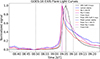 |
Figure 1. Normalized multi-wavelength light curve of an M1.0 solar flare observed on 2024-07-31. The plot displays simultaneous emissions of SXR (black), Lyman-alpha (blue), He II (red), and the Mg II index (purple). The vertical dashed lines mark the start, peak, and end times of the emissions. |
4 Results
4.1 Peak contrast of EUV
To determine whether all the flares exhibited enhancements in the EUV spectral lines relative to the background level, we determined the peak contrast. This measure quantified the percentage increase in the EUV spectral line flux during the flare compared to its pre-flare background. A large enhancement indicates that the flare produced a strong increase in the irradiance of the specific spectral line, while a low or negligible contrast implies that the flare had little to no effect on the EUV emission of that line. We calculated the peak contrast in equation (1):
 (1)
(1)
Each EUV spectral line showed a significant enhancement above the background for almost all 1022 flares analyzed. The top row of Figure 2 shows that the He II (30.4 nm) line exhibited a positive intensity enhancement for all analyzed X-class flare events, indicating that its irradiance increased relative to pre-flare levels in every case. These enhancements typically ranged from about 0.8% to 40%, indicating that many flares produced substantially stronger He II emission. In the most energetic cases, the contrast reached approximately 65% and 78%. According to the GOES-16 database, the flare with a 65% increase corresponds to an X14.6 event, while the 78% enhancement is associated with an X8.9 flare. These exceptionally powerful events occurred at helioprojective coordinates (x, y)=(484.4, −278.6) and (37.8, −380.7), respectively. It should be noted that there is some uncertainty regarding the X14.6 event, as other databases list it as an X9.3 flare. Although these observed enhancements are not corrected for center-to-limb effects, which might have reduced their apparent magnitude, their high GOES class indicates a very powerful energy release that still results in a significant signal above background. Overall, these results indicate that the He II emission closely reflects the physical conditions associated with flare energy release, with the strongest events producing the largest relative increases in intensity. For M-class flares, He II enhancements typically ranged from about 0.3% to 20%. Enhancements exceeding 20% were strongly associated with X-class flares, as only about 1% of M-class events reached such levels. X-class flares produce enhancements in Lyman-alpha ranging from 0.1% to 12%. Most M-class flares exhibit increases of approximately 0.5–5% above the background, with fewer than 1% reaching 20–25% enhancement. The Mg II index shows the smallest relative increase, ranging from 0.1% to 5% for X-class flares and around 0.1–2.5%, for M-class flares. Although these flare-related changes are small in magnitude, the Mg II index is measured with high instrumental stability and low relative uncertainty, allowing such variations to be robustly detected (McClintock et al. 2025). The Mg II line cores undergo several absorption and scattering processes before their emission escapes the solar atmosphere, which limits the observed intensity increase. Photons may be reabsorbed or re-emitted by the surrounding plasma, reducing their direct contribution to the measured signal. The two Mg II emission cores, h and k, form at slightly different heights in the chromosphere due to their differing oscillator strengths. Because these heights correspond to distinct atmospheric layers, variations in energy deposition during flares can modify the relative intensity ratio of the h and k lines. Some flares deposit less energy at particular chromospheric heights, producing measurable changes in the h/k ratio (Roy & Tripathi 2024). Lyman-alpha emission is likewise reduced by radiative transfer effects. Much of the emitted radiation is reabsorbed by overlying hydrogen before escaping the solar atmosphere, which limits the observed flare-driven enhancement. Lyman-alpha also has a very high quiet-Sun background, further reducing the relative contrast during flares. To characterize this background variability, we measured the rotational modulation of solar Lyman-alpha using GOES-16/EUVS irradiance. The data were grouped by Carrington rotation (27.3 days), and the variability for each rotation was calculated using equation (2), where I is the Lyman-alpha irradiance. This analysis was carried out over the declining phase of Solar Cycle 24 (12 January 2017 to 15 November 2019) and the rising phase of Solar Cycle 25 (12 December 2019 to 25 May 2025). The mean rotational variability was 23.12% for Cycle 24 and 22.13% for Cycle 25.
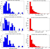 |
Figure 2. (Left) Percentage increase of EUV for X-class flares above background. (Right) Percentage increase of EUV for M-class flares above background. |
 (2)
(2)
Among the three EUV spectral lines examined, the He II line exhibits the largest enhancement relative to the background as shown in Table 1. Because He II undergoes comparatively little reabsorption, its emission more directly reflects the local plasma conditions during flare energy release (Vial 1982a). Rapid heating of the transition region during flares produces steep temperature gradients that strongly amplify emission in lines formed at those heights, such as He II.
Summary of EUV spectral line enhancements for M- and X-class flares. Values are percent increases relative to pre-flare background.
4.2 Durations
Understanding the temporal characteristics of flare events helps interpret their physical properties and energy release mechanisms. In this section, we describe how we determine the durations of solar flares using both SXR and EUV observations. We calculate the SXR durations as the difference between the flare end time and start time provided by GOES. The end time of the SXR flare is defined as the moment when its intensity decays to half of its peak value. For each flare, we calculate the EUV durations by measuring the time between the start of its longest continuous rising phase in the background-subtracted EUV flux and the moment when that flux declines to half of its peak value. Figure 3 compares the durations of SXR emissions with those of the three EUV emission lines (Lyman-alpha, He II, and the Mg II index) for both M- and X-class solar flares. To provide a more complete statistical picture, the relationships were quantified using Pearson’s linear correlation (r), Spearman’s rank correlation (ρ), Kendall’s tau (τ), and the coefficient of determination (R2). For X-class flares, all three EUV lines display strong and statistically significant positive correlations with SXR durations, suggesting that longer X-ray flares generally coincide with longer EUV emission times. The highest correlation is found for He II (r = 0.72, ρ = 0.76, τ = 0.59, R2 = 0.52), followed by Lyman-alpha (r = 0.63, ρ = 0.65, τ = 0.49, R2 = 0.39) and the Mg II index (r = 0.67, ρ = 0.66, τ = 0.50, R2 = 0.45). Although there is some scatter, especially for longer duration events, the overall trend is monotonic and consistent. This means that in X-class flares, the processes of energy release and cooling tend to follow a predictable pattern.
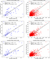 |
Figure 3. Scatter plots showing the correlation between flare durations in the SXR and durations in the EUV: He II (30.4 nm), Lyman-alpha, and the Mg II index. (Left) Represents X-class flares, (Right) represents M-class flares. Linear regression fits (solid black lines) are shown with their best-fit equations and correlation coefficients (r). The results indicate that both flare classes show positive correlations between SXR durations and chromospheric/transition-region emissions, with generally stronger correlations for X-class events. |
In contrast, M-class flares exhibit much greater variability in their EUV durations relative to SXR. The correlation strengths are noticeably weaker with He II (r = 0.63, ρ = 0.42, τ = 0.30, R 2 = 0.39), Lyman-alpha (r = 0.49, ρ = 0.30, τ = 0.21, R 2 = 0.24) and Mg II index (r = 0.48, ρ = 0.34, τ = 0.23, R 2 = 0.23). The distribution of points on the right side of Figure 3 shows that many M-class events cluster at short durations, while others extend to longer SXR times, but correspond to disproportionately weak or short EUV responses. This broad spread indicates that the relationship between SXR and EUV emission times for M-class flares is nonlinear and highly variable, likely reflecting differences in flare morphology, loop geometry, chromospheric heating, and optical-depth effects that influence EUV line formation. The Pearson correlation coefficients for the durations are summarized in Table 2. Overall, these results suggest that X-class flares show a relatively consistent relationship between the durations of SXR and EUV emissions, whereas M-class flares are much less predictable, with EUV responses varying widely even for similar SXR durations. Among the EUV lines, He II shows the most statistically consistent behavior across correlation measures. The significant scatter, especially among M-class flares, shows how important it is to account for complex, nonlinear effects and physical differences when interpreting how SXR and EUV durations relate. On average, the EUV emissions peak several minutes before the SXR maximum, indicating that chromospheric heating occurs early in the flare evolution. The mean lead times are summarized in Table 3.
Statistical measurements of correlation (r) between EUV emissions and SXR parameters.
Sample size, mean lead time, 95% confidence intervals, range, and standard deviation of EUV emission peak times relative to the SXR peak for M- and X-class flares.
4.3 Peak fluxes
Figure 4 presents a scatter plot illustrating the relationship between the peak flux of solar flares in SXR and in the EUV spectral line He II, shown here as an example. This approach builds on the work of Milligan et al. (2020), who demonstrated a relationship between SXR peak flux and Lyman-alpha emissions for M- and X-class flares. Our analysis extends this framework by including additional EUV spectral lines, He II, and the Mg II index, alongside Lyman-alpha. The data reveal several useful thresholds. For instance, when He II peaks below 10−4 W m−2, the likelihood of the flare being classified as an X-class event decreases significantly. Similarly, a He II peak below 10−5 W m−2 corresponds to a reduced likelihood of an M-class event. Lyman-alpha and the Mg II index shows similar behavior. These thresholds indicate that stronger SXR flares are generally accompanied by stronger enhancements in EUV emissions. However, substantial scatter is evident, particularly among M-class flares. Many of these events show similar SXR fluxes but very different EUV intensities, indicating that the efficiency of energy transport and radiation in the lower atmosphere varies from flare to flare. Previous studies support this behavior. Lyman-alpha and SXR contribute differently to the flare energy budget and upper-atmospheric forcing. Milligan et al. (2012) found that Lyman-alpha emitted about twice as much energy as SXR during an X-class flare, and (Kretzschmar 2017) reported Lyman-alpha fluences up to an order of magnitude larger than SXR across roughly one hundred events. Our results are consistent with these findings. In most M-class flares, Lyman-alpha, He II, and Mg II peaks exceed their SXR counterparts by factors of several to tens, while X-class flares show smaller ratios because of stronger coronal heating and ionization boost the SXR output. Thus, the broad scatter in our peak-peak relationships is expected and reflects the distinct physical processes traced by EUV and SXR emissions. Despite these threshold patterns, the correlation strength differs among the EUV lines. The correlation between Lyman-alpha and SXR peak fluxes are relatively weak (r = 0.32). In contrast, He II shows a stronger correlation with SXR (r = 0.53), while Mg II displays an intermediate value (r = 0.43). Table 2 summarizes these correlations. In Figure 4, the slope of the lower edge of the distribution for M-class and X-class flares appears noticeably steeper than that of the upper edge. This behavior likely reflects that the He II emission does not increase as strongly as the SXR flux between small and large flares. At higher flare energies, a larger fraction of the released energy is radiated in hotter coronal lines, while He II becomes less sensitive to further heating due to ionization in the transition region. Additionally, the strong imbalance in sample sizes, with far more M-class flares than X-class events, likely biases the overall correlation. The clustering of numerous moderate flares along the lower envelope disproportionately influences the fitted trend relative to the sparsely sampled high-energy end.
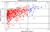 |
Figure 4. Scatter plot comparing the peak of background-subtracted He II flux and SXR intensities for Type I flares. The He II and SXR values span multiple orders of magnitude, highlighting the relationship between chromospheric and coronal energy release during flare events. This plot is similar to the one in Milligan et al. (2020) for Lyman-alpha. |
4.4 Behavior of the EUV spectral lines relative to SXR
We examined whether EUV spectral lines respond consistently with SXR emissions during flares. In Figure 5, the left panels show the differences in peak flux between SXR and He II versus SXR and Lyman-alpha, while the right panels show the corresponding differences in peak times. We quantified the main timing trend and marked flares with deviations larger than ±1σ as outliers (stars). This analysis includes all flares meeting criteria (1) – (3), not just Type I events. For M-class flares (top left panel), peak fluxes of He II and Lyman-alpha show a roughly linear relationship with SXR, with more scatter at lower fluxes. X-class flares (bottom left panel) display a similar pattern, indicating that both lines respond comparably to SXR intensity. A similar trend is observed between Lyman-alpha and the Mg II index for both flare classes. In the timing panels (right), many flares follow a roughly linear trend, but some deviate (the stars). This is because a given flare does not always fall into the same temporal classification across all EUV lines; for example, a Type I Lyman-alpha flare is not always a Type I He II flare. These outlier flares (stars) show no clear pattern in strength, duration, or solar disk location.
5 Discussion and conclusion
This paper examined how different EUV emissions, Lyman-alpha, He II (30.4 nm), and the Mg II index measured by EUVS, relates to SXR emissions during solar flares. Our goal was to determine whether these EUV signals could provide early warnings of SXR flare intensity and duration. Consistent with previous studies (Jing et al. 2020), we found that the EUV emissions typically peaked shortly before the SXR maximum, providing a brief but measurable lead time. This behavior is consistent with the rapid chromospheric heating driven by nonthermal electrons before the coronal SXR peak, in agreement with earlier work on Lyman-alpha flare emission (e.g., Nusinov et al. 2006; Rubio da Costa et al. 2009; Milligan & Chamberlin 2016). However, this early EUV peak occurred in only about two-thirds of the events (74% for Lyman-alpha, 75% for He II, and 72% for the Mg II index). In the remaining flares, the EUV peak coincided with or followed the SXR peak, indicating that the lead time is not universally available. These differences likely reflect variations in how energy is released and transported during individual events. Thus, while the lead time is promising for forecasting; it cannot be assumed for all flares. The typical lead time of 4–5 min is short but operationally useful, as it provides an indication that the SXR emission is approaching its maximum. Such early cues may improve situational awareness for satellite operations, communications, and power systems affected by enhanced ionization. Integrating EUV-based diagnostics into real-time monitoring could therefore strengthen space weather nowcasting. An operational system could exploit this behavior by monitoring EUV and SXR irradiance for the occurrence of an EUV peak during the SXR rise phase. The empirical relationships presented here could then be used to estimate the SXR peak properties, excluding cases in which the SXR peak occurs earlier.
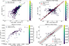 |
Figure 5. (Left) The difference in flux between the spectral lines illustrates whether they behave similarly in terms of intensity with respect to SXR. (Right) The difference in peak times shows whether Lyman-alpha and He II exhibit similar timing relative to the SXR emission. The top panels correspond to M-class flares, and the bottom panels to X-class flares. The red and blue dots represent flares where Lyman-alpha and He II belong to the same flare Type, while the black dots indicate flares that do not share the same classification across all EUV lines. |
Our analysis used the one-minute averaged EUV and SXR irradiances provided by NOAA, although both quantities are measured at one-second cadence by EXIS. Higher cadence data are available to operational users and would enable more refined real-time applications. The relationships between SXR and EUV peak fluxes showed only weak correlations across all spectral lines, suggesting that flare energy is not uniformly distributed throughout the solar atmosphere. Although intensity thresholds, for example, the absence of X-class events with He II peaks below 10−5 W m−2, indicate that EUV emissions broadly scale with flare strength, the large scatter implies complex and nonlinear coupling between the chromosphere and corona. Among the EUV lines, He II exhibited the highest, though still modest, correlation with SXR (r = 0.53). Lyman-alpha and Mg II showed even weaker relationships, likely due to strong opacity effects and radiative transfer processes. These results extend those of Milligan et al. (2020), reinforcing that while EUV emissions provide insight into flare energetics, their diagnostic reliability is limited by atmospheric complexity.
The comparison of SXR and EUV durations further illustrated how energy couples through atmospheric layers. X-class flares showed strong correlations, indicating well-synchronized heating and cooling across wavelengths. We interpret this synchronicity as a consequence of the significantly higher thermal energies and emission measures in X-class flares compared to M-class flares (Ryan et al. 2012; Aschwanden et al. 2015). These greater energies drive more vigorous chromospheric evaporation and the formation of denser coronal loops, which subsequently cool in a coordinated fashion. The enhanced densities extend the radiative cooling phase, a standard result from flare cooling theory, so that both the SXR and EUV emissions decay on comparable timescales (e.g., as applied and observed by Veronig et al. 2002). This coupling results in SXR and transition region durations tracking one another closely. M-class flares, however, exhibited weaker and more scattered relationships. Based on a detailed analysis of a C-class flare event, Wang et al. (2026) demonstrated that the lower plasma densities characteristic of smaller flares favor cooling dominated by thermal conduction rather than radiative losses. This naturally introduces a scaling with flare energy: For smaller flares, conductive cooling becomes so efficient that it disrupts the normal flow of heat from the super-hot SXR plasma down to the cooler EUV-emitting layers. This disruption weakens the classic Neupert relationship, making the timing connection between the emissions more scattered and less predictable. In conduction-dominated regimes, the plasma is driven below the SXR temperature sensitivity is faster than it can produce substantial transition region emission, effectively decoupling their temporal evolution. Additional factors, such as loop topology, heating efficiency, and multi-threaded activation, likely contribute to the observed scatter (Warren 2006). Across all classes, the He II line displayed the most consistent temporal behavior among the EUV diagnostics, supporting its effectiveness as an indicator of energy deposition in the transition region. This is consistent with the line’s formation during chromospheric evaporation and its sensitivity to downward-directed conduction fronts during the flare decay.
Although this work did not introduce new analytical techniques, it advances our understanding of how EUV and SXR emissions are temporally and energetically linked. It highlights where EUV lines, particularly He II, can assist in flare prediction, and where their reliability is limited. Future studies using larger high cadence datasets and improved statistical methods would help quantify these relationships more robustly. Overall, EUV emissions offer valuable, though imperfect, insight into flare timing and strength and can contribute to improved monitoring of solar activity and mitigation of space weather impacts. Lastly, while the EUV lines examined here generally exhibit similar behavior relative to SXR, their differing opacities, formation heights, and response times indicate that each probes a distinct atmospheric layer and physical process. Consequently, no single EUV line can fully capture flare evolution, and a multi-line approach is essential for a comprehensive assessment of energy release and transport during solar flares.
Acknowledgments
The authors would like to thank Dr. Janet Machol (NOAA/NCEI) for her help in understanding the NOAA data processing algorithms and the GOES-R team at the University of Colorado/LASP for their advice on the design of the EXIS instruments. We would also like to thank the reviewers for their comments. Their suggestions have improved the manuscript. The editor thanks Matthew DeLand and an anonymous reviewer for their assistance in evaluating this paper.
Funding
This work was supported by the South African National Research Foundation (NRF) through two grants: AM was supported by a student bursary from SANSA, MS was supported by the SARChI grant to SANSA.
Data availability statement
The data used in this article are from the National Oceanic and Atmospheric Administration (NOAA) web page. We used the GOES-16 level two, science quality data, one-minute averages. Downloaded from: EUVS: https://data.ngdc.noaa.gov/platforms/solar-space-observing-satellites/goes/goes16/l2/data/euvs-l2-avg1m_science/ and XRS: https://data.ngdc.noaa.gov/platforms/solar-space-observing-satellites/goes/goes16/l2/data/xrsf-l2-avg1mscience/
References
- Aschwanden MJ. 2004. Physics of the solar Corona: an introduction, Springer, Berlin, Heidelberg. https://doi.org/10.1007/3-540-30766-4. [Google Scholar]
- Aschwanden MJ, Boerner P, Ryan D, Caspi A, McTiernan JM, et al. 2015. Global energetics of solar flares. II. Thermal energies. Astrophys J 802(1): 53. https://doi.org/10.1088/0004-637X/802/1/53. [Google Scholar]
- Bekker S, Milligan RO, Ryakhovsky IA. 2024. The influence of different phases of a solar flare on changes in the total electron content in the earth’s ionosphere. Astrophys J 971(2): 188. https://doi.org/10.3847/1538-4357/ad631d. [Google Scholar]
- Bhatnagar A, Livingston W. 2005. Fundamentals of solar astronomy. World Sci 6: 167–178. https://doi.org/10.1142/5171. [Google Scholar]
- Brekke P, Rottman G, Fontenla J, Judge P. 1996. The ultraviolet spectrum of a 3B class flare observed with SOLSTICE. Astrophys J 468: 418. https://doi.org/10.1086/177701. [Google Scholar]
- Carmichael H. 1964. A Process for Flares. In: AAS–NASA Symposium on the Physics of Solar Flares, Hess WN (Ed.), vol. 50 of NASA Special Publication, NASA, Washington, DC, pp. 451–456. [Google Scholar]
- Cebula R, DeLand M, Schlesinger B. 1992. Estimates of solar variability using the solar backscatter ultraviolet (SBUV) 2 Mg II index from the NOAA 9 satellite. J Geophys Res: Atmosp 97(D11): 11,613–11,620. https://doi.org/10.1029/92JD00893. [Google Scholar]
- Curdt W, Brekke P, Feldman U, Wilhelm K, Dwivedi B, et al. 2001. The SUMER spectral atlas of solar-disk features. Astron Astrophys 375(2): 591–613. https://doi.org/10.1051/0004-6361:20010364. [Google Scholar]
- Eparvier F, Crotser D, Jones A, McClintock W, Snow M, et al. 2009. The extreme ultraviolet sensor (EUVS) for GOES-R. In: Solar physics and space weather instrumentation III, vol. 7438, SPIE, pp. 31–38. https://doi.org/10.1117/12.826445. [Google Scholar]
- Fang H, Wang S, Sheng Z. 2012. HF waves heating ionosphere F-layer. Chin Sci Bull 57(31): 4036–4042. https://doi.org/10.1007/s11434-012-5408-4. [Google Scholar]
- Fletcher L, Dennis B, Hudson H, Krucker S, Phillips K, et al. 2011. An observational overview of solar flares. Space Sci Rev 159: 19–106. https://doi.org/10.1007/s11214-010-9701-8. [Google Scholar]
- Gold T, Hoyle F. 1960. On the origin of solar flares. Mon Not Roy Astron Soc 120(2): 89–105. https://doi.org/10.1093/mnras/120.2.89. [Google Scholar]
- Goodman S, Schmit T, Daniels J, Redmon R. 2019. The GOES-R series: A new generation of geostationary environmental satellites. Elsevier. https://doi.org/10.1016/B978-0-12-814327-8.00023-8. [Google Scholar]
- Gosling J, Asbridge J, Bame S, Feldman W. 1976. Solar wind speed variations: 1962–1974. J Geophys Res 81(28): 5061–5070. https://doi.org/10.1029/JA081i028p05061. [Google Scholar]
- Greatorex H, Milligan R, Chamberlin P. 2023. Observational analysis of Lyα emission in equivalent-magnitude solar flares. Astrophys J 954(2): 120. https://doi.org/10.3847/1538-4357/acea7f. [Google Scholar]
- Guyer S, Can Z. 2013. Solar flare effects on the ionosphere. In: 2013 6th International conference on recent advances in space technologies (RAST), IEEE, pp. 729–733. https://doi.org/10.1109/RAST.2013.6581305. [Google Scholar]
- Handzo R, Forbes J, Reinisch B. 2014. Ionospheric electron density response to solar flares as viewed by Digisondes. Space Weather 12(4): 205–216. https://doi.org/10.1002/2013SW001020. [Google Scholar]
- Heath D, Schlesinger B. 1986. The Mg 280-nm doublet as a monitor of changes in solar ultraviolet irradiance. J Geophys Res: Atmosp 91(D8): 8672–8682. https://doi.org/10.1029/JD091iD08p08672. [Google Scholar]
- Hirayama T. 1974. Theoretical model of flares and prominences: I: Evaporating flare model. Sol Phys 34: 323–338. https://doi.org/10.1007/BF00153671. [Google Scholar]
- Hudson, H., 1972. Thick-target processes and white-light flares. Sol Phys 24: 414–428. https://doi.org/10.1007/BF00153384. [Google Scholar]
- Hudson H. 2011. Global properties of solar flares. Space Sci Rev: 158(1): 5–41. https://doi.org/10.1007/s11214-010-9721-4. [Google Scholar]
- Jafari A, Vishniac E. 2018. Introduction to magnetic reconnection. https://doi.org/10.48550/arXiv.1805.01347. [Google Scholar]
- Jing Z, Pan W, Yang Y, Song D, Tian J, et al. 2020. The Lyα emission in solar flares. I. A statistical study on its relationship with the 1–8 Å Soft X-ray emission. Astrophys J 904(1): 41. https://doi.org/10.3847/1538-4357/abbacc. [Google Scholar]
- Kerr G, Simões P, Qiu J, Fletcher L. 2015. IRIS observations of the Mg ii h and k lines during a solar flare. Astron Astrophys 582: A50. https://doi.org/10.1051/0004-6361/201526128. [Google Scholar]
- Kopp R, Pneuman G. 1976. Magnetic reconnection in the corona and the loop prominence phenomenon. Sol Phys 50: 85–98. https://doi.org/10.1007/BF00206193. [Google Scholar]
- Kretzschmar M. 2017. Temperature dependence of the flare fluence scaling exponent. In: Solar and stellar flares, Springer, pp. 215–231. https://doi.org/10.1007/s11207-015-0783-z. [Google Scholar]
- Le H, Liu L, Chen Y, Wan W. 2013. Statistical analysis of ionospheric responses to solar flares in the solar cycle 23. J Geophys Res: Space Phys 118(1): 576–582. https://doi.org/10.1029/2012JA017934. [Google Scholar]
- Li N, Ding Z, Chen J, Xu Z. 2012. Analysis of ionospheric response to solar flares at Kunming site. In: ISAPE2012, IEEE, pp. 547–550. https://doi.org/10.1109/ISAPE.2012.6408829. [Google Scholar]
- Li Y, Li Q, Song D, Battaglia A, Xiao H, et al. 2022. The Lyα Emission in a C1. 4 Solar Flare Observed by the Extreme Ultraviolet Imager aboard Solar Orbiter. Astrophys J 936(2): 142. https://doi.org/10.3847/1538-4357/ac897c. [Google Scholar]
- Machol J, Codrescu S, Peck C. 2021. User’s Guide for GOES-R XRS L2 Products. https://data.ngdc.noaa.gov/platforms/solar-spaceobserving-satellites/goes/goes16/l2/docs/GOES-R_XRS_L2_Data_Users_Guide.pdf. [Google Scholar]
- Machol JL, Eparvier FG, Viereck RA, Woodraska DL, Snow M, et al., 2020. Chapter 19 – GOES-R Series Solar X-ray and Ultraviolet Irradiance. In: The GOES-R Series, Goodman SJ, Schmit TJ, Daniels J, Redmon RJ. (Eds.), Elsevier, pp. 233–242. ISBN 978-0-12-814327-8. https://doi.org/10.1016/B978-0-12-814327-8.00019-6. https://www.sciencedirect.com/science/article/pii/B9780128143278000196. [Google Scholar]
- MacQueen R, Fisher R. 1983. The kinematics of solar inner coronal transients. Sol Phys 89: 89–102. https://doi.org/10.1007/BF00211955. [Google Scholar]
- McClintock WE, Snow M, Crotser D, Eparvier FG. 2025. High precision, high time-cadence measurements of the Mg II index of solar activity by the GOES-R Extreme Ultraviolet Irradiance Sensor 1: EUVS-C design and preflight calibration. J Space Weather Space Clim 15: 12. https://doi.org/10.1051/swsc/2025005. [Google Scholar]
- McClintock WE, Snow M, Eden TD, Eparvier FG, Machol JL, et al. 2025. High precision, high time-cadence measurements of the MgII index of solar activity by the GOES-R Extreme Ultraviolet Irradiance Sensor 2: EUVS-C initial flight performance. J Space Weather Space Clim. https://doi.org/10.1051/swsc/2025006. [Google Scholar]
- Milligan R. 2021. Solar irradiance variability due to solar flares observed in Lyman-alpha emission. Sol Phys 296(3): 51. https://doi.org/10.1007/s11207-021-01796-3. [Google Scholar]
- Milligan R, Chamberlin P. 2016. Anomalous temporal behaviour of broadband Lyα observations during solar flares from SDO/EVE. Astron Astrophys 587: A123. https://doi.org/10.1051/0004-6361/201526682. [Google Scholar]
- Milligan R, Hudson H, Chamberlin P, Hannah I, Hayes L. 2020. Lyman-alpha variability during solar flares over solar cycle 24 using GOES-15/EUVS-E. Space Weather 18(7): e2019SW002,331. https://doi.org/10.1029/2019SW002331. [Google Scholar]
- Milligan RO, Chamberlin PC, Hudson HS, Woods TN, Mathioudakis M, et al. 2012. Observations of Enhanced Extreme Ultraviolet Continua during an X-Class Solar Flare Using SDO/EVE. Astrophys J Lett 748(1): L14. https://doi.org/10.1088/2041-8205/748/1/L14. [Google Scholar]
- Milligan RO, Dennis BR. 2009. Velocity characteristics of evaporated plasma using Hinode/EUV imaging spectrometer. Astrophys J 699(2): 968. https://doi.org/10.1088/0004-637X/699/2/968. [Google Scholar]
- Mthethwa A. 2024. Can Geostationary Operational Environmental Satellite (GOES) Ultraviolet Measurements Predict the X-ray Properties of Flares?, Master’s thesis, University of Johannesburg, Johannesburg, South Africa. https://ujcontent.uj.ac.za/esploro/outputs/graduate/Can-geostationary-operational-environmental-satellite-GOES/9955190007691. [Google Scholar]
- Neupert W, 1968. Comparison of solar X-ray line emission with microwave emission during flares. Astrophys J 153: L59. https://doi.org/10.1086/180220. [Google Scholar]
- Nusinov A, Kazachevskaya T, Kuznetsov S, Myagkova I, Yushkov BY. 2006. Ultraviolet, hard X-ray, and gamma-ray emission of solar flares recorded by VUSS-L and SONG instruments in 2001–2003. Sol System Res 40: 282–285. https://doi.org/10.1134/S0038094606040034. [Google Scholar]
- O’Hare AN, Bekker S, Greatorex HJ, Milligan RO. 2025. Investigating a Characteristic Time Lag in the Ionospheric F-Region’s Response to Solar Flares. Atmosphere 16(8): 937. https://doi.org/10.3390/atmos16080937. [Google Scholar]
- Panos B. 2021. The analysis of solar flares using machine learning. Ph.D. Thesis, University of Geneva, Switzerland. https://doi.org/10.13097/archive-ouverte/unige:153812. [Google Scholar]
- Qian L, Burns A, Chamberlin P, Solomon S. 2011. Variability of thermosphere and ionosphere responses to solar flares. J Geophys Res: Space Phys 116(A10): 13. https://doi.org/10.1029/2011JA016777. [Google Scholar]
- Qian L, Wang, W, Burns, AG, Chamberlin, PC, Coster, A, Zhang, S-R, Solomon, SC. 2019. Solar flare and geomagnetic storm effects on the thermosphere and ionosphere during 6–11 September 2017. J Geophys Res: Space Phys 124(3): 2298–2311. [Google Scholar]
- Roy S, Tripathi D. 2024. Evolution of the ratio of Mg ii intensities during solar flares. Astrophys J 964(2): 106. https://doi.org/10.3847/1538-4357/ad2a46. [Google Scholar]
- Rubio da Costa F, Fletcher L, Labrosse N, Zuccarello F. 2009. Observations of a solar flare and filament eruption in Lyman and X-rays. Astron Astrophys 507(2): 1005–1014. https://doi.org/10.1051/0004-6361/200912651. [Google Scholar]
- Ryan DF, Milligan RO, Gallagher PT, Dennis BR, Tolbert AK, et al. 2012. The thermal properties of solar flares over three solar cycles using GOES X-ray observations. Astrophys J Suppl Ser 202(2): 11. https://doi.org/10.1088/0067-0049/202/2/11. [Google Scholar]
- Silva A, Wang H, Gary D, Nitta N, Zirin H. 1997. Imaging the chromospheric evaporation of the 1994 June 30 solar flare. Astrophys J 481(2): 978. https://doi.org/10.1086/304076. [Google Scholar]
- Snow M, Machol J, Viereck R, Woods T, Weber M, et al. 2019. A Revised Magnesium II Core-to-Wing Ratio From SORCE SOLSTICE. Earth Space Sci 6(11): 2106–2114. https://doi.org/10.1029/2019EA000652. [CrossRef] [Google Scholar]
- Sturrock P. 1966. Model of the high-energy phase of solar flares. Nature 211(5050): 695–697. https://doi.org/10.1038/211695a0. [Google Scholar]
- Tandberg-Hanssen E, Emslie A. 1988. The physics of solar flares, Cambridge University Press, 14. https://doi.org/10.1126/science.245.4919.770.a. [Google Scholar]
- Thiemann EM, Eparvier FG, Woods TN. 2017. A time dependent relation between EUV solar flare light-curves from lines with differing formation temperatures. J Space Weather Space Clim 7: A36. https://doi.org/10.1051/swsc/2017037. [Google Scholar]
- Tsurutani B, Verkhoglyadova O, Mannucci A, Lakhina G, Li G. et al. 2009. A brief review of “solar flare effects” on the ionosphere. Radio Sci 44(01): 1–14. https://doi.org/10.1029/2008RS004029. [Google Scholar]
- Veronig A, Vršnak B, Temmer M, Hanslmeier A. 2002. Relative timing of solar flares observed at different wavelengths. Solar Phys 208(2): 297–315. https://doi.org/10.1023/A:1020563804164. [Google Scholar]
- Vial J. 1982a. Optically thick lines in a quiescent prominence-Profiles of Lyman-alpha, Lyman-beta/HI/, K and H/Mg II/, and K and H/Ca II/lines with the OSO 8 LPSP instrument. Astrophys J 253: 330–352. https://doi.org/10.1086/159639. [Google Scholar]
- Vial J. 1982b. Two-dimensional nonlocal thermodynamic equilibrium transfer computations of resonance lines in quiescent prominences. Astrophys J 254: 780–795. https://doi.org/10.1086/159789. [Google Scholar]
- Wang Y, Mulay SM, Fletcher L. 2026. Extremely energetic EUV late phase of a pair of C-class flares caused by a non-eruptive sigmoid. arXiv preprint arXiv:2512.08324, 16. https://doi.org/10.48550/arXiv.2512.08324. [Google Scholar]
- Warren HP. 2006. Multithread hydrodynamic modeling of a solar flare. Astrophys J 637(1): 522. https://doi.org/10.1086/497904. [CrossRef] [Google Scholar]
- Woods T, Eparvier F, Fontenla J, Harder J, Kopp G, et al. 2004. Solar irradiance variability during the October 2003 solar storm period. Geophys Res Lett 31(10): 2. https://doi.org/10.1029/2004GL019571. [Google Scholar]
- Woods T, Rottman G, White O, Fontenla J, Avrett E. 1995. The solar Ly-alpha line profile. Astrophys J 442: 898–906. https://doi.org/10.1086/175492. [Google Scholar]
- Woods T, Tobiska W, Rottman G, Worden J. 2000. Improved solar Lyman α irradiance modeling from 1947 through 1999 based on UARS observations. J Geophys Res: Space Phys 105(A12): 27,195–27,215. https://doi.org/10.1029/2000JA000051. [Google Scholar]
- Woods TN, Eden T, Eparvier FG, Jones AR, Woodraska DL, et al. 2024. GOES-R Series X-Ray Sensor (XRS): 1. Design and pre-flight calibration. J Geophys Res: Space Phys 129(11): e2024JA032,925. https://doi.org/10.1029/2024JA032925. [Google Scholar]
Cite this article as: Mthethwa A. and Snow M. 2026. Using solar ultraviolet irradiance measurements from GOES/EXIS to nowcast flare X-ray properties. J. Space Weather Space Clim. 16, 12. https://doi.org/10.1051/swsc/2026010.
All Tables
Summary of EUV spectral line enhancements for M- and X-class flares. Values are percent increases relative to pre-flare background.
Statistical measurements of correlation (r) between EUV emissions and SXR parameters.
Sample size, mean lead time, 95% confidence intervals, range, and standard deviation of EUV emission peak times relative to the SXR peak for M- and X-class flares.
All Figures
|
Figure 1. Normalized multi-wavelength light curve of an M1.0 solar flare observed on 2024-07-31. The plot displays simultaneous emissions of SXR (black), Lyman-alpha (blue), He II (red), and the Mg II index (purple). The vertical dashed lines mark the start, peak, and end times of the emissions. |
| In the text | |
|
Figure 2. (Left) Percentage increase of EUV for X-class flares above background. (Right) Percentage increase of EUV for M-class flares above background. |
| In the text | |
|
Figure 3. Scatter plots showing the correlation between flare durations in the SXR and durations in the EUV: He II (30.4 nm), Lyman-alpha, and the Mg II index. (Left) Represents X-class flares, (Right) represents M-class flares. Linear regression fits (solid black lines) are shown with their best-fit equations and correlation coefficients (r). The results indicate that both flare classes show positive correlations between SXR durations and chromospheric/transition-region emissions, with generally stronger correlations for X-class events. |
| In the text | |
|
Figure 4. Scatter plot comparing the peak of background-subtracted He II flux and SXR intensities for Type I flares. The He II and SXR values span multiple orders of magnitude, highlighting the relationship between chromospheric and coronal energy release during flare events. This plot is similar to the one in Milligan et al. (2020) for Lyman-alpha. |
| In the text | |
|
Figure 5. (Left) The difference in flux between the spectral lines illustrates whether they behave similarly in terms of intensity with respect to SXR. (Right) The difference in peak times shows whether Lyman-alpha and He II exhibit similar timing relative to the SXR emission. The top panels correspond to M-class flares, and the bottom panels to X-class flares. The red and blue dots represent flares where Lyman-alpha and He II belong to the same flare Type, while the black dots indicate flares that do not share the same classification across all EUV lines. |
| In the text | |
Current usage metrics show cumulative count of Article Views (full-text article views including HTML views, PDF and ePub downloads, according to the available data) and Abstracts Views on Vision4Press platform.
Data correspond to usage on the plateform after 2015. The current usage metrics is available 48-96 hours after online publication and is updated daily on week days.
Initial download of the metrics may take a while.