| Issue |
J. Space Weather Space Clim.
Volume 16, 2026
Topical Issue - Space Climate: Solar Extremes, Long-Term Variability, and Impacts on Earth’s System
|
|
|---|---|---|
| Article Number | 11 | |
| Number of page(s) | 10 | |
| DOI | https://doi.org/10.1051/swsc/2026009 | |
| Published online | 07 May 2026 | |
Research Article
A new deep-learning approach to infer solar and geomagnetic parameters for the 1859 Carrington event
1
Center for Solar-Terrestrial Research, New Jersey Institute of Technology, Newark, NJ 07102, USA
2
Institute for Space Weather Sciences, New Jersey Institute of Technology, Newark, NJ 07102, USA
3
Solar-Terrestrial Centre of Excellence – SIDC, Royal Observatory of Belgium, Ringlaan -3- Av. Circulaire 1180, Brussels, Belgium
4
Centre for Mathematical Plasma Astrophysics, Department of Mathematics, KU Leuven, Celestijnenlaan 200B 3001, Leuven, Belgium
5
Division of Space Information Research, Korea Astronomy and Space Science Institute, Daejeon 34055, Republic of Korea
6
School of Space Research, Kyung Hee University, Yongin 17104, Republic of Korea
7
G-LAMP NEXUS Institute, Kyung Hee University, Yongin 17104, Republic of Korea
8
Institute for Space-Earth Environmental Research, Nagoya University, Nagoya
4648601, Japan
* Corresponding author: This email address is being protected from spambots. You need JavaScript enabled to view it.
Received:
27
September
2025
Accepted:
10
March
2026
Abstract
In this study, we investigate the solar and geomagnetic parameters of the 1859 Carrington event using deep learning and empirical relationships. For this, we apply an image translation model, a popular deep learning method based on conditional Generative Adversarial Networks, to the generation of magnetograms from sunspot drawings. We train the model using pairs of sunspot data from Debrecen Photoheliographic Data and their corresponding Solar and Heliospheric Observatory/Michelson Doppler Imager (SOHO/MDI) and Solar Dynamics Observatory/Helioseismic and Magnetic Imager (SDO/HMI) magnetograms from 1996 to 2018, using data from January–July and December of each year for training and data from August and November for validation. To test the model, we compare actual magnetograms with artificial-intelligence-based (AI-based) ones for September and October. Our results show that the unsigned magnetic fluxes of AI-based magnetograms closely match those of the originals. Applying this model to Carrington’s full-disk sunspot drawing of 1 September 1859, we generate an AI-based magnetogram and estimate its unsigned magnetic flux. To estimate solar and geomagnetic parameters, we use the following empirical relationships: magnetic flux and flare peak flux, magnetic flux and coronal mass ejection (CME) speed, CME speed and transit time, CME speed and interplanetary coronal mass ejection (ICME) speed, and ICME speed and the Disturbance Storm Time (Dst) index to obtain upper-limit estimates for an extreme event. We find that the estimated Sun-Earth transit time is 16.7 h, consistent with the historical observations. The corresponding Dst value is about −1313 nT, which is broadly consistent with previous reconstruction-based estimates for the Carrington storm.
Key words: Space weather / Solar extreme event / Geomagnetic storms / Historical observations / Deep learning
© H. Lee et al. Published by EDP Sciences 2026
 This is an Open Access article distributed under the terms of the Creative Commons Attribution License (https://creativecommons.org/licenses/by/4.0), which permits unrestricted use, distribution, and reproduction in any medium, provided the original work is properly cited.
1 Introduction
Large solar eruptions, such as solar flares and coronal mass ejections (CMEs), occur in magnetically complex active regions that often host large sunspot groups. These eruptions can significantly impact the near-Earth space environment (Pulkkinen 2007; Cliver et al. 2022; Usoskin et al. 2023). In particular, the solar storm associated with the Carrington event in 1859 resulted in one of the most powerful geomagnetic storms in recorded history and extremely disturbed the terrestrial magnetosphere (Tsurutani et al. 2003; Cliver & Dietrich 2013; Hayakawa et al. 2019, 2022). Richard Carrington’s observations of this event have marked one of the first recorded instances of a white-light flare (Carrington 1859; Hodgson 1859) and have remained vital data for quantifying this extreme solar and geomagnetic storm (Cliver & Dietrich 2013; Cliver et al. 2022; Hayakawa et al. 2022, 2023).
Carrington’s sunspot drawings around the Carrington event have been an essential source for discussions in solar physics. This event has been treated as a benchmark for such extreme solar and geomagnetic storms (Cliver et al. 2022; Usoskin et al. 2023). It is important to develop studies on such extreme solar and geomagnetic storms, as these historical records provide crucial insights into extreme solar storms that can cause enormous economic loss (Oughton et al. 2017; Cliver et al. 2022; Hudson et al. 2024).
We have multiple magnitude estimates for the Carrington flare. Some studies used the sunspot group area to estimate the upper limit of the bolometric energy that the source active region could accommodate. Hayakawa et al. (2016) and Watari (2022) used equation (1) of Shibata et al. (2013) for the relationship between the area of sunspot groups and the upper limit of the expected flare energy to estimate the Carrington flare to be about 4 × 1033 erg and X36, respectively. We have to be slightly cautious about their estimates, as they are an order of magnitude different.
Carrington’s records provide even more direct details for the flare magnitude estimate. Hayakawa et al. (2023) estimated the area of the white-light flaring region of the Carrington event and its blackbody brightness temperature. Then they estimated the Carrington flare magnitude of ∼X80 (X46–X126) from the combination of their reconstructions for the area, duration, and temperature of the Carrington flare based on the original records.
Several authors used geomagnetic records for indirect magnitude estimates. These authors estimated the flare intensity of the Carrington event to be about X45 (±5) from the relationship between the amplitude of the perturbation change in the Earth’s magnetic field caused by the solar flare effect (Cliver & Svalgaard 2004; Boteler 2006; Cliver & Dietrich 2013; Curto et al. 2016). This estimation has been revised to ∼X105 (X81–X146) in Hudson et al. (2025) on the basis of the GOES rescaling (Cliver et al. 2022) and the revised geomagnetic data (Beggan et al. 2024). This result is broadly consistent with the direct estimate from Hayakawa et al. (2023).
Thus, these different methods suggest that the magnitude of the Carrington flare was between X46–X126 and X81–X146. We conservatively take the overlap between these two estimates, to narrow the range to X81–X126. These values are much larger than any solar flare ever recorded during modern times, even after accounting for the GOES-satellite recalibration (Hudson et al. 2024).
In addition, several studies have quantified the resultant geomagnetic storm in terms of the Disturbance Storm Time (Dst) index and H-component values of the Carrington event from Colaba Observatory in India. Tsurutani et al. (2003) estimated the Dst of approximately −1760 nT on the basis of the Colaba storm decay timescale, the CME transit time, and auroral visibility sites, and compared their results with the local geomagnetic disturbance in Colaba, while Love & Mursula (2024) found this estimate not reproducible from their equations, assumptions, and input parameters. Li et al. (2006), using solar wind reconstructions, estimated the H-component depression of −1600 nT using the same data. Siscoe et al. (2006) provided a more conservative estimate of −850 nT, based on a visual hourly average of the Colaba data in the figure shown by Tsurutani et al. (2003), following the definition of the Dst index. Gonzalez et al. (2011) also used hourly averages and estimated the peak Dst at −1150 nT. Cliver & Dietrich (2013) estimated the Dst value between −850 and −1150 nT, using visual hourly averages of the Colaba data. Hayakawa et al. (2022) located the Colaba yearbook to revise the local H component, derive the local Y and Z components, reconstruct the Sq variations, and estimated the local Dst as −918 nT to −979 nT.
In contrast, the spatial evolution of the Carrington active region has attracted less attention. The snapshot drawing of Carrington (1859) has been contextualised to the whole-disk sunspot drawings from multiple observers and the sequential temporal evolutions only quite recently (Hayakawa et al. 2019). This difficulty might be overcome with the recent development of artificial intelligence (AI) tools. The advancements in AI and deep learning technologies have opened new avenues for analyzing such historical solar sunspot drawings and reconstructing the solar magnetic activity at that time. Zheng et al. (2016) employed a convolutional neural network to recognize handwritten characters in scanned sunspot drawings. These drawings, provided by the Yunnan Observatory of the Chinese Academy of Sciences, were used to determine full-disk sunspot numbers and areas. Xu et al. (2021) introduced a deep-learning method for segmenting sunspot components from Purple Mountain Astronomical Observatory sunspot drawings. This technique separately extracts the numbers and areas of pores, spots, umbras, and penumbras. Lee et al. (2021) applied deep learning techniques to generate modern satellite-like solar data from Galileo Galilei’s sunspot drawings and then estimated the related physical parameters.
In this paper, we propose to infer solar and geomagnetic parameters of the Carrington event by applying a deep learning model to its sunspot drawing. We generate AI-based magnetograms from Carrington sunspot drawings using deep learning and calculate their unsigned magnetic flux. Based on the inferred unsigned magnetic flux, we estimate the associated flare class and CME speed. Subsequently, these values allow us to infer the interplanetary CME (ICME) speed and the Dst value from the statistical relationships between them for extreme events. This approach provides new insights into the Carrington event and highlights the potential of using historical sunspot observations to study the solar-terrestrial interactions of extreme events.
This study is organized as follows: Section 2 describes the data used in this analysis, and Section 3 outlines the methodology. Section 4 presents the results and discussion, while Section 5 gives a summary and conclusions.
2 Data
We use the Debrecen Photoheliographic Data (DPD) sunspot catalog (Baranyi et al. 2016; Győri et al. 2017) for input data. We make DPD-based sunspot drawings using only the sunspot’s position and area information to generate an AI-based magnetogram. This approach allows us to infer the magnetic field strength with minimal information when reconstructing historical sunspot drawings. Sunspots are represented by ellipses, approximating their appearance as projections of circles on a sphere onto a plane. The center of the resulting ellipse corresponds to the visible center of the sunspot, and its area represents the total projected area of the sunspot. For a detailed process, see the left panel of Figure 1 in Baranyi et al. (2016). Then, we convert the catalog information into a single-channel grayscale input image with three levels (Figs. 1a and 1d). In this representation, pixels inside the DPD sunspot area are set to 255, pixels on the solar disk outside the sunspot area are set to 127, and pixels outside the solar disk are set to 0. In other words, we use a simple three-level discrete encoding in which 127 represents a mid-gray background level for the quiet solar disk. The reason why sunspots are expressed in a circular shape is to use the uniform sunspot information provided by DPD from 1874 to 2018 in the deep learning model.
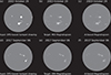 |
Figure 1. Comparison between MDI/HMI magnetograms and AI-based ones on 2003 October 29 (top), and 2017 September 6 (bottom). Panels (a) and (d) show schematic sunspot drawings constructed from the DPD catalog (DPD-based sunspot drawings), which are used as input to the model. Panels (b) and (e) show the corresponding observed MDI/HMI magnetograms as targets, and panels (c) and (f) show the AI-based magnetograms from our model. The magnetograms in (b), (c), (e), and (f) are byte-scaled to | ± 1000| G for display only. |
We use the Solar and Heliospheric Observatory (Domingo et al. 1995, SOHO)/Michelson Doppler Imager (Scherrer et al. 1995, MDI) and Solar Dynamics Observatory (Pesnell et al. 2012, SDO)/Helioseismic and Magnetic Imager (Schou et al. 2012, HMI) for target data. We make level 1.5 images by calibrating, rotating, and centering from the line-of-sight magnetogram FITS files. In order to use the MDI (1996–2010) and HMI (2011–2018) data together, the MDI magnetic field values are corrected using the equation MDI = −0.18 + 1.40 × HMI of Liu et al. (2012). We consider the magnetic flux density to be within ±3000 Gauss, a typical valid range for the line-of-sight (LoS) magnetic field measurements in SDO/HMI magnetograms (Hoeksema et al. 2014). We calculate the flux only within 0.95 solar radii. As sunspot drawings represent only strong magnetic fields, we calculate the total unsigned magnetic fluxes for areas with absolute field strengths exceeding 30 Gauss-approximately three times the noise levels (Liu et al. 2012).
We use only the magnetogram data observed within ±48 min (0.44° in heliospheric longitude) of each DPD sunspot drawing’s observation time to minimize the effect of solar rotation. Additionally, we standardize the solar disk size to align the DPD sunspot drawing with the magnetogram and downsample the image to 512 × 512 pixels. The total dataset comprises 6965 pairs of DPD-based sunspot drawings and magnetograms, covering May 1996 to June 2018. For training, we use 4733 pairs from January to July and December of each year. For validation, we use 1151 pairs from August and November. The test set consists of 1081 pairs from 1996 to 2017, only data from September and October. This month-wise split introduces about a one-month gap between the training and test periods and helps reduce data leakage from long-lived active regions. This period was chosen because the publicly available DPD dataset currently provides sunspot data up to mid-2018. Thus, our dataset range spans the MDI and HMI eras, ensuring consistent pairing with high-quality magnetogram observations.
For the application of our model, we use the full-disk sunspot drawing for 1859 September 1, based on Carrington’s original manuscript (RAS MS Carrington 3.2, f. 313a; Image courtesy of the Royal Astronomical Society) and reproduced as Figure 2 in Hayakawa et al. (2019), after removing the background (Fig. 2a). We used Carrington’s original manuscript, as Carrington (1859) only published a snapshot of the specific active region and missed the whole-disk presentation. Carrington’s sunspot drawing is a hand-made sketch on a projected solar disk, whereas the DPD-based input is generated from the DPD sunspot catalog. As a result, the spot shapes, intensity patterns, and disk geometry are not identical between the two data sets. To apply our model, we convert Carrington’s drawing into a DPD-style image: we align the solar disk, map the spot outlines to heliographic coordinates, and resample them onto the same 512 × 512 grid as the DPD images while preserving the spot positions and areas (Fig. 2b). This procedure reduces the domain gap between the historical and modern data, although some residual systematic differences may remain. The original sunspot area ranges from 2970 (Hayakawa et al. 2023), to 3000 (Hayakawa et al. 2016; Watari 2022), and 3100 (Meadows 2024) millionths of the Sun’s visible hemisphere (MSH) in previous studies. The stylised sunspot area in the DPD sunspot drawing format is almost at the upper edge of this range, at 3103 MSH (Fig. 2c), probably due to the transformation and stylisation to the DPD format. Then, we generate the input image in the three-level format following the process used for the training and test data (Fig. 3a).
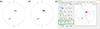 |
Figure 2. Pre-processing to transform the original Carrington sunspot drawing into a DPD-style sunspot drawing. (a) Full-disk Carrington sunspot drawing (from Hayakawa et al. 2019) after the removal of the background. (b) DPD-style Carrington sunspot drawing. (c) Area measurement of the Carrington sunspot drawing, marked with a green box in the Helio Viewer software (https://www.petermeadows.com/html/software.html). |
 |
Figure 3. DPD-style Carrington sunspot drawing (a) and the corresponding AI-based magnetogram (b) on 1 September 1859. |
We also use additional solar and geomagnetic data sets to derive the empirical relationships used later in this study. For the relation between the magnetic fluxes and flare peak fluxes, the magnetic fluxes are calculated daily at 00:00 UT from ARs located within ±60° of the central meridian of the Sun. This calculation employs the MTOT keyword, which represents the total line-of-sight magnetic flux density, a standard parameter provided in both the MDI Tracked Active Region Patches and the Spaceweather HMI Active Region Patch data sets. For MDI data, MTOT values are calibrated by applying the correction factor derived by Liu et al. (2012) and adjusting for the resolution differences between MDI and HMI to ensure consistency in flux measurements. The flare peak fluxes correspond to the strongest Geostationary Operational Environmental Satellite (GOES) X-ray flare that occurred within 24 h in the corresponding Active Regions (ARs). The pre-2016 GOES flare peak fluxes are rescaled based on the intercalibration proposed by Hudson et al. (2024). For the relation between the magnetic fluxes and CME speeds, the CME speeds are taken from the Coordinated Data Analysis Workshop (CDAW) SOHO/Large Angle and Spectrometric Coronagraph (LASCO; Brueckner et al. 1995) Halo CME (HCME) catalog1. We only consider front-side halo CMEs heading toward the Earth, which are known to produce strong geomagnetic storms (Gosling et al. 1990; Srivastava & Venkatakrishnan 2004). The corresponding ICME speeds and minimum Dst values are obtained from the ICME lists by Cane & Richardson (2003) and Richardson & Cane (2010).
3 Method
We use the pix2pixHD model introduced by Wang et al. (2017), which enables high-resolution image-to-image translation and is an extension of the original pix2pix model (Isola et al. 2016). This model uses a conditional Generative Adversarial Network (Mirza & Osindero 2014) to learn mappings between paired image domains, producing highly realistic images. We consider pix2pixHD more suitable for our research than pix2pix, as we work with data such as magnetograms where structural detail is needed.
The model consists of a global generator and a multi-scale discriminator. The generator takes a single-channel 512 × 512 DPD image as input and produces a magnetogram of the same dimensions. It follows an encoder–bottleneck–decoder structure: the encoder progressively downsamples the input while extracting features, a series of residual blocks refines the representation at the bottleneck, and the decoder upsamples back to the original resolution to produce the output magnetogram.
The multi-scale discriminator evaluates the realism of the generated magnetograms at different spatial scales. Three discriminators independently assess the concatenated input–output pair at the original resolution and at two progressively downsampled resolutions. This multi-scale design encourages the generator to produce outputs that are consistent in both local fine-scale details and global large-scale structure.
The generator is trained with a combination of an adversarial loss and a feature-matching loss. The adversarial loss follows the least-squares GAN (LSGAN; Mao et al. 2016) formulation:
![Mathematical equation: $$ \begin{aligned}&L_D = \frac{1}{2} \, \mathbb{E} \left[||D(x, y) - 1 ||_2^2\right] + \frac{1}{2} \, \mathbb{E} \left[||D(x, G(x)) ||_2^2\right], \end{aligned} $$](/articles/swsc/full_html/2026/01/swsc250084/swsc250084-eq1.gif) (1)
(1)
![Mathematical equation: $$ \begin{aligned}&L_{\mathrm{GAN} } = \mathbb{E} \left[||D(x, G(x)) - 1 ||_2^2\right], \end{aligned} $$](/articles/swsc/full_html/2026/01/swsc250084/swsc250084-eq2.gif) (2)
(2)
where x denotes the input DPD image, y the real magnetogram, G(x) the generated magnetogram, and D the discriminator. The feature-matching loss stabilizes training by minimizing the L 1 distance between intermediate feature representations of real and generated images extracted from each discriminator layer and scale:
 (3)
(3)
where k indexes the discriminator scale and i the layer. The total generator loss is
 (4)
(4)
with λ = 10. Both the generator and discriminator are optimized using the Adam optimizer (Kingma & Ba 2014) with a learning rate of 2 × 10⁻⁴, β 1 = 0.5, and β 2 = 0.999. Following the pix2pixHD training protocol of Wang et al. (2017), the learning rate is held constant for the first 100 epochs and then linearly decayed to zero over the remaining 100 epochs, for a total of 200 training epochs.
We first train a model to generate solar magnetograms like MDI/HMI from DPD-based sunspot drawings, using the DPD-magnetogram pairs and the train/validation/test split described in Section 2. The model is trained for 200 epochs following the pix2pixHD training protocol, using the validation set to monitor performance and select the final checkpoint, while the test set is kept unseen during training and used only for the final evaluation. Then, we apply this trained model to Carrington’s sunspot drawing, generating an AI-based magnetogram of the Carrington event. From this magnetogram, we infer the solar and geomagnetic parameters of the 1859 Carrington event.
4 Results and discussion
We generate AI-based magnetograms from DPD-based sunspot drawings. Figure 1 shows a comparison between MDI/HMI magnetograms and AI-based ones for the two strongest events from the past solar cycles: (1) National Oceanic and Atmospheric Administration (NOAA) AR 10486 that produced one of the strongest flares of Solar Cycle 23 on October 29, 2003, (2) NOAA AR 12673 that produced the strongest flare of Solar Cycle 24 on September 6, 2017. The comparisons between the target and the AI-based magnetograms indicate that the structural characteristics of the AI-based ones are quite similar to those of the original ones. Additionally, the unsigned magnetic fluxes of the AI-based ones are consistent with those of the original ones. This demonstrates that our deep learning model effectively estimates unsigned flux. The results indicate that the model captures key information on AR size and location from the DPD-based sunspot drawings, which is sufficient for estimating the total unsigned magnetic flux. At the same time, the AI-based magnetograms are not free from artifacts. Visual inspection shows that the model sometimes smooths sharp sunspot boundaries and occasionally produces faint spurious features in the quiet Sun. Minor shape distortions can also appear near the solar limb, where projection and foreshortening effects are strongest.
We estimate the total unsigned magnetic flux of both AI-based and original ones for the test data, with their temporal variations shown in Figure 4a. To avoid uncertainties near the limb, we only consider pixels within 0.95 solar radii for all images. The average correlation coefficient (CC) of the total unsigned magnetic flux between the generated and original ones is 0.95 (Fig. 4b), indicating that the model accurately reproduces the unsigned magnetic fluxes of ARs, regardless of solar activity. The percentage error of the total unsigned magnetic flux is 17%. As an example from the test period, the prominent peak in late October 2014 occurs during the passage of a very large sunspot group associated with NOAA AR 12192. At this time, the AI-based magnetogram reproduces the overall extent of the main group and gives a total unsigned flux similar to that derived from the corresponding SDO/HMI magnetogram. This shows that the model also works for test cases with sunspot groups comparable in size to our estimate for the Carrington sunspot region.
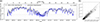 |
Figure 4. Total unsigned magnetic flux of both original and AI-based ones for the test set. (a) Temporal variations of the total unsigned magnetic flux. The bottom x-axis shows the observation date (year-month) for each DPD test image, while the top x-axis indicates the corresponding image index in the test set (from 1 to N), sorted in time. The black solid line shows variations from the original magnetograms and the blue solid line corresponds to those from the AI-based ones. (b) Scatter plot between the total unsigned magnetic fluxes of the original and AI-based magnetograms. |
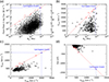 |
Figure 5. Solar and geomagnetic activities from empirical relationships: (a) flare peak flux vs. magnetic flux, (b) CME speed vs. magnetic flux, (c) ICME speed vs. CME speed, (d) Dst value vs. ICME speed. Red dotted lines show the linear fittings from the red diamonds corresponding to each group’s most extreme value. The estimates of the Carrington event are shown in blue triangles. |
We apply our model to Carrington’s sunspot drawing and generate the corresponding HMI-like magnetogram, shown in Figure 3b for 1 September 1859. We calculate the unsigned magnetic flux (7.5 × 10²² Mx) in the Carrington sunspot group from the generated magnetogram. Then we estimate the solar and geomagnetic parameters from several empirical relationships (Fig. 5). We consider total magnetic flux, flare peak flux, CME speed, ICME speed, and Dst value for each AR from April 1996 to May 2021. The upper panels of Figure 5 reflect empirical relationships for the sunspot magnetic flux with the upper limits of the expected flare peak X-ray flux (a) and the expected CME velocity (b). The lower panels of Figure 5 reflect empirical relationships for the CME speed with the upper limits of the expected ICME speed (c) and the expected negative Dst excursion (d).
Figure 5a shows the relationship between magnetic fluxes and flare peak fluxes. The X-axis data are divided into ten groups with the same data numbers, and only the data with the strongest flare flux value in each group (red diamond in Fig. 5a) is used for linear fitting (red dashed line in Fig. 5a). We consider only these maximum values because the Carrington event is known to be an extreme case, and our goal is to estimate an upper limit for its flare peak flux. The GOES flare catalog is incomplete for weaker events, which contributes to the under-populated lower-right part of the point distribution (Wheatland 2000). However, when we repeat the fit using only M- and X-class flares, the resulting slope and intercept are very similar to those obtained from our original maximum-value fit, and the extrapolated flare peak flux for the Carrington event changes only marginally, well within our overall uncertainties. This suggests that the upper envelope we use for the Carrington estimate, is not strongly affected by the incompleteness of weak GOES events. From this relationship, the GOES X-ray flare class of the Carrington event can be estimated to be X25 in terms of the upper limit. Our upper-envelope estimate (X25) is smaller than some previous reconstructions (X46–X146; Cliver & Svalgaard 2004; Boteler 2006; Cliver & Dietrich 2013; Curto et al. 2016; Cliver et al. 2022; Hayakawa et al. 2023; Hudson et al. 2025), although it overlaps with the reported range when uncertainties are considered. To estimate the uncertainty associated with the predicted flare class obtained from the linear regression model, we utilized the covariance matrix returned by the LINFIT procedure in the Interactive Data Language (IDL). This matrix provides the standard errors of the fitted regression coefficients. The 1-σ uncertainty interval for the prediction spans from approximately X3 to X240.
Our estimation of the Carrington flare class has limitations in predicting extreme events, as it relies solely on the peak flux of the strongest flares observed in the last two solar cycles. The strongest flare in the last two solar cycles was on 4 November 2003, with a flare class of X43.2, according to the recent intercalibrations of Hudson et al. (2024), although this event occurred outside the ±60° range from the central meridian of the Sun. Within ±60°, the strongest flare was X24 on 28 October 2003.
Figure 5b shows the relationship between the total unsigned magnetic fluxes and the CME speeds. Because the number of events is relatively small, we divide the X-axis data into five groups with equal number of events and, in each group, select the event with the fastest CME speed (red diamonds in Fig. 5b). We then perform a linear fit using only these upper-envelope points (red dashed line in Fig. 5b). From this relationship, the upper-limit CME speed of the Carrington event is estimated to be 3007 ± 52 km s−1, with the uncertainty estimated using the same approach as for the flare class. This CME speed corresponds to an estimated Sun-Earth transit time of about 16.7 h according to the empirical formula (T = 76.86 − 0.02 × V CME) given by Kim et al. (2007). Interestingly, this estimate is close to the reported intervals of ∼17.6 h and ≤17.1 h between the flare and the storm onset (Cliver & Dietrich 2013; Hayakawa et al. 2022). Independently of this empirical framework, we note that the CME speed of the Carrington event can also be estimated directly from the observed Sun-Earth transit time. If one adopts a delay of about 17−18 h between the flare and the onset of the geomagnetic storm (Cliver & Dietrich 2013; Hayakawa et al. 2022) and a nominal Sun-Earth distance of 1 AU, a simple kinematic estimate yields a CME speed of about 2400 km s−1.
Figures 5c and 5d show two relationships of CME speed with the upper limits of the expected ICME speed and the most negative Dst excursions. The X-axis data are divided into five groups with the same data numbers, and only the data with the fastest ICME speed in each group (red diamond in Fig. 5c) are used for linear fitting (red dashed line in Fig. 5c). In the same way, only the data with the lowest Dst values in each group (red diamond in Fig. 5d) are used for linear fitting (red dashed line in Fig. 5d). From these relationships, the ICME speed and Dst value of the Carrington event can be estimated to be 1476 ± 45 km s−1 and −1313 ± 102 nT, with the uncertainty estimated using the same approach as for the flare class. Our approximation of the Dst value is broadly consistent with the existing estimates (Cliver & Dietrich 2013; Hayakawa et al. 2022). Our method is a new approach to infer the Dst value of the most powerful geomagnetic storms in history.
Magnetic flux is an important factor for producing energetic flares and CMEs, but it does not uniquely determine their peak emission or dynamical properties. Other properties of the active region, such as magnetic shear, topology, helicity, and the pre-eruptive configuration, also play important roles. As a result, the empirical relationships that we derive between total unsigned flux and flare peak flux, CME speed, ICME speed, and Dst exhibit substantial scatter and are best interpreted as upper-envelope trends rather than deterministic laws. In applying these relations to the 1859 Carrington event, we assume that the event was extremely strong, as indicated by independent evidence such as reports of low-latitude aurora and large magnetometer deflections. Under this assumption, our estimates provide plausible upper bounds on the associated solar and geomagnetic parameters. For other historical events where the level of extremity is not well constrained by independent observations, our flux-based empirical relations alone cannot uniquely determine the true flare, CME, or geomagnetic intensity and should be used together with additional observational or proxy information.
In addition to these conceptual limitations, our estimates also inherit uncertainties from the multi-step inference chain used to obtain the parameters of the Carrington event. First, the unsigned magnetic flux is reconstructed from the historical drawing by the deep-learning model, which introduces a finite error compared with modern test magnetograms. Second, this reconstructed flux is then propagated through successive empirical relationships linking flux to CME speed, CME speed to ICME speed, and ICME speed to Dst value, each step adding statistical and modeling uncertainty. In practice, the CME speed, ICME speed, and Dst value that we infer for the Carrington event should therefore not be regarded as precise point values, but as approximate estimates that reflect the combined uncertainties from both the reconstruction and the subsequent scaling relations.
5 Summary and conclusion
In this study, we propose a new approach to investigate the solar and geomagnetic parameters of the 1859 Carrington event using deep learning. This framework is intended to provide an empirical upper bound for exceptionally extreme events rather than a best estimate for typical conditions. For this, we trained a deep learning model to generate HMI-like magnetograms from DPD-based emulated drawings. Our model demonstrates the consistency of the unsigned magnetic fluxes between target and AI-based magnetograms for the test data set, with a mean CC of 0.95 and a percentage error of 17%. Applying our model to Carrington’s 1859 sunspot drawing, we generate an AI-based magnetogram of the Carrington event, which enables us to estimate key solar and geomagnetic parameters. By examining the relationship between magnetic flux and flare peak flux, we estimate the Carrington flare class to be approximately X25 (X3–X240) in the upper limit. Similarly, we estimate the Carrington CME speed at 3007 ± 52 km s−1, which gives the Sun-Earth transit time (about 16.7 h) according to the empirical formula of Kim et al. (2007). It is interesting to note that this value is consistent with the real observation time (about 17.6 or ≤17.1 h). Our analysis is extended to derive its ICME speed and Dst value, yielding our upper-limit estimates of 1476 ± 45 km s−1 and −1313 ± 102 nT, respectively. Both the CME transit time and the inferred storm magnitude are broadly consistent with ranges reported in previous studies, and should be interpreted as approximate upper-bound estimates given the scatter of the empirical relations. These results suggest that our approach provides a novel method to reconstruct solar and geomagnetic parameters and shows that physical estimates based on sunspot data are physically consistent with historical geomagnetic reports. This study may help improve our understanding of extreme solar and geomagnetic events, contributing to better preparedness for future space weather events.
Acknowledgments
We thank the reviewers and the editor for their helpful comments that improved the manuscript. We thank all the observers who made the drawings of sunspots. We also thank the numerous team members who have contributed to the success of the SOHO (Domingo et al. 1995) and SDO (Pesnell et al. 2012) missions. HH thanks Baranyi Tunde and Ludmány Andras for establishing the DPD database and allowing access, Petrovay Kristóf for his help on his visit to Hungary, and Sian Prosser of the Royal Astronomical Society for letting him consult and study Carrington’s original manuscripts. The editor thanks Subhamoy Chatterjee and an anonymous reviewer for their assistance in evaluating this paper.
Funding
HL was supported by NASA grants 80NSSC24M0174 and 80NSSC24K0843 and U.S. NSF grants OAC-2504860 and OAC-2320147. DL was supported by a Senior Research Project (G088021N) of the FWO Vlaanderen, the Belgian Federal Science Policy Office (BELSPO) through the contract B2/223/P1/CLOSE-UP, and thanks the BELSPO for the provision of financial support in the framework of the PRODEX Programme of the European Space Agency under contract number 4000143743. EP was supported by the Basic Science Research Program through the NRF, funded by the MoE (RS-2024-00337363). YM was supported by funding from the Korean government (KASA, Korea AeroSpace Administration, grant number RS-2023-00234488, Development of Solar Synoptic Magnetograms Using Deep Learning), the Korea Astronomy and Space Science Institute under the R&D program (Project No. 2026183005) supervised by the Ministry of Science and ICT (MSIT), BK21 FOUR program through National Research Foundation of Korea (NRF) under the Ministry of Education (MoE) (Kyung Hee University, Human Education Team for the Next Generation of Space Exploration), Global-Learning & Academic research institution for Master’s • PhD students, and Postdocs (G-LAMP) Program of the National Research Foundation of Korea (NRF) grant funded by the Ministry of Education (RS-2025-25442355). HH was supported by JSPS Grant-in-Aids JP25K17436 and JP25H00635, the ISEE director’s leadership fund for FYs 2021 – 2025, the Young Leader Cultivation (YLC) programme of Nagoya University, Tokai Pathways to Global Excellence (Nagoya University) of the Strategic Professional Development Program for Young Researchers (MEXT), and the young researcher units for the advancement of new and undeveloped fields in Nagoya University Program for Research Enhancement, and the NIHU Multidisciplinary Collaborative Research Projects NINJAL unit “Rediscovery of Citizen Science Culture in the Regions and Today”.
Conflict of interest
The authors declare no conflict of interest.
Data availability statement
The sunspot data used in this study are available from the Debrecen Photoheliographic Data sunspot catalog (Baranyi et al. 2016; Győri et al. 2017) via https://fenyi.solarobs.epss.hun-ren.hu/en/databases/DPD/. The Carrington sunspot drawing data are available from Hayakawa et al. (2019) and the drawing is reproduced with permission from the Royal Astronomical Society (MS Carrington 3.2, f. 313a). The SOHO/MDI and SDO/HMI magnetograms are available from the Joint Science Operations Center (JSOC) at https://jsoc.stanford.edu/ (data can be accessed via the JSOC search/export interface). Magnetic fluxes used in this study are taken from the Space-Weather MDI Active Region Patches (SMARPs; JSOC DRMS series mdi.smarp_96m; Bobra et al. 2021) and the Space-weather HMI Active Region Patch (SHARP; JSOC DRMS series hmi.sharp_720s; Bobra et al. 2014) data series. GOES soft X-ray fluxes (XRS) were obtained from the NOAA NCEI GOES Space Environment Monitor (SEM) science-quality reprocessed XRS archive (GOES-1 through -15) available via https://www.ncei.noaa.gov/products/goes-1-15/space-weather-instruments and direct download at https://www.ncei.noaa.gov/data/goes-space-environment-monitor/access/. CME speeds are taken from the CDAW SOHO/Large Angle and Spectrometric Coronagraph (LASCO; Brueckner et al. 1995) HCME catalog at https://cdaw.gsfc.nasa.gov/CME_list/halo/halo.html. ICME speeds and minimum Dst values are obtained from the ICME lists by Cane & Richardson (2003) and Richardson & Cane (2010) at https://izw1.caltech.edu/ACE/ASC/DATA/level3/icmetable2.htm.
References
- Baranyi T, Győri L, Ludmány A. 2016. On-line tools for solar data compiled at the debrecen observatory and their extensions with the greenwich sunspot data. Sol Phys 291(9–10): 3081–3102. https://doi.org/10.1007/s11207-016-0930-1. [CrossRef] [Google Scholar]
- Beggan CD, Clarke E, Lawrence E, Eaton E, Williamson J, et al. 2024. Digitized continuous magnetic recordings for the August/September 1859 storms from London, UK. Space Weather 22(3): e2023SW003807. https://doi.org/10.1029/2023SW003807. [Google Scholar]
- Bobra MG, Sun X, Hoeksema JT, Turmon M, Liu Y, et al. 2014. The Helioseismic and Magnetic Imager (HMI) Vector Magnetic Field Pipeline: SHARPs – Space-Weather HMI Active Region Patches. Sol Phys 289(9): 3549–3578. https://doi.org/10.1007/s11207-014-0529-3. [Google Scholar]
- Bobra MG, Wright PJ, Sun X, Turmon MJ. 2021. SMARPs and SHARPs: Two solar cycles of active region data. Astrophys J Suppl Ser 256(2): 26. https://doi.org/10.3847/1538-4365/ac1f1d. [Google Scholar]
- Boteler DH. 2006. The super storms of August/September 1859 and their effects on the telegraph system. Adv Space Res 38(2): 159–172. https://doi.org/10.1016/j.asr.2006.01.013. [CrossRef] [Google Scholar]
- Brueckner GE, Howard RA, Koomen MJ, Korendyke CM, Michels DJ, et al. 1995. The Large Angle Spectroscopic Coronagraph (LASCO). Sol Phys 162(1–2): 357–402. https://doi.org/10.1007/BF00733434. [CrossRef] [Google Scholar]
- Cane HV, Richardson IG. 2003. Interplanetary coronal mass ejections in the near-Earth solar wind during 1996–2002. J Geophys Res (Space Phys) 108(A4): 1156. https://doi.org/10.1029/2002JA009817. [Google Scholar]
- Carrington RC. 1859. Description of a singular appearance seen in the Sun on September 1, 1859. Mon Notices Roy Astron Soc 45: 13–15. https://doi.org/10.1093/mnras/20.1.13. [Google Scholar]
- Cliver EW, Dietrich WF. 2013. The 1859 space weather event revisited: Limits of extreme activity. J Space Weather Space Clim 45: A31. https://doi.org/10.1051/swsc/2013053. [Google Scholar]
- Cliver EW, Svalgaard L. 2004. The 1859 solar-terrestrial disturbance and the current limits of extreme space weather activity. Sol Phys 224(1–2): 407–422. https://doi.org/10.1007/s11207-005-4980-z. [CrossRef] [Google Scholar]
- Cliver EW, Schrijver CJ, Shibata K, Usoskin IG. 2022. Extreme solar events. Liv Rev Sol Phys 19(1): 2. https://doi.org/10.1007/s41116-022-00033-8. [Google Scholar]
- Curto JJ, Castell J, Del Moral F. 2016. Sfe: Waiting for the big one. J Space Weather Space Clim 45: A23. https://doi.org/10.1051/swsc/2016018. [Google Scholar]
- Domingo V, Fleck B, Poland AI. 1995. The SOHO mission: An overview. Sol Phys 162(1–2): 1–37. https://doi.org/10.1007/BF00733425. [CrossRef] [Google Scholar]
- Gonzalez WD, Echer E, Clúa de Gonzalez AL, Tsurutani BT, Lakhina GS. 2011. Extreme geomagnetic storms, recent Gleissberg cycles and space era-superintense storms. J Atmos Solar-Terr Phys 73(11–12): 1447–1453. https://doi.org/10.1016/j.jastp.2010.07.023. [Google Scholar]
- Gosling JT, Bame SJ, McComas DJ, Phillips JL. 1990. Coronal mass ejections and large geomagnetic storms. Geophys Res Lett 17(7): 901–904. https://doi.org/10.1029/GL017i007p00901. [Google Scholar]
- Győri L, Ludmány A, Baranyi T. 2017. Comparative analysis of Debrecen sunspot catalogues. Mon Notices Roy Astron Soc 465(2): 1259–1273. https://doi.org/10.1093/mnras/stw2667. [Google Scholar]
- Hayakawa H, Iwahashi K, Tamazawa H, Isobe H, Kataoka R, et al. 2016. East Asian observations of low-latitude aurora during the Carrington magnetic storm. Publ Astron Soc Japan 68(6): 99. https://doi.org/10.1093/pasj/psw097. [Google Scholar]
- Hayakawa H, Ebihara Y, Willis DM, Toriumi S, Iju T, et al. 2019. Temporal and spatial evolutions of a large sunspot group and great auroral storms around the Carrington event in 1859. Space Weather 17(11): 1553–1569. https://doi.org/10.1029/2019SW002269. [CrossRef] [Google Scholar]
- Hayakawa H, Nevanlinna H, Blake SP, Ebihara Y, Bhaskar AT, et al. 2022. Temporal variations of the three geomagnetic field components at colaba observatory around the Carrington storm in 1859. Astrophys J 928(1): 32. https://doi.org/10.3847/1538-4357/ac2601. [CrossRef] [Google Scholar]
- Hayakawa H, Bechet S, Clette F, Hudson HS, Maehara H, et al. 2023. Magnitude estimates for the Carrington flare in 1859 september: As seen from the original records. Astrophys J 954(1): L3. https://doi.org/10.3847/2041-8213/acd853. [Google Scholar]
- Hodgson R. 1859. On a curious appearance seen in the Sun. Mon Notices Roy Astron Soc 45: 15–16. https://doi.org/10.1093/mnras/20.1.15a. [Google Scholar]
- Hoeksema JT, Liu Y, Hayashi K, Sun X, Schou J, et al. 2014. The Helioseismic and Magnetic Imager (HMI) vector magnetic field pipeline: Overview and performance. Sol Phys 289(9): 3483–3530. https://doi.org/10.1007/s11207-014-0516-8. [Google Scholar]
- Hudson H, Cliver E, White S, Machol J, Peck C, et al. 2024. The greatest GOES soft X-ray flares: Saturation and recalibration over two hale cycles. Sol Phys 299(3): 39. https://doi.org/10.1007/s11207-024-02287-x. [Google Scholar]
- Hudson HS, Cliver EW, Hayakawa H, Beggan CD, Clarke E, et al. 2025. The X-ray class of the Carrington flare. Mon Notices Roy Astron Soc 544(2): 1992–1998. https://doi.org/10.1093/mnras/staf967. [Google Scholar]
- Isola P, Zhu JY, Zhou T, Efros AA. 2016. Image-to-image translation with conditional adversarial networks. Preprint. https://doi.org/10.48550/arXiv.1611.07004. [Google Scholar]
- Kim KH, Moon YJ, Cho KS. 2007. Prediction of the 1-AU arrival times of CME-associated interplanetary shocks: Evaluation of an empirical interplanetary shock propagation model. J Geophys Res (Space Phys) 112(A5): A05104. https://doi.org/10.1029/2006JA011904. [Google Scholar]
- Kingma DP, Ba J. 2014. Adam: A method for stochastic optimization. Preprint. https://doi.org/10.48550/arXiv.1412.6980. [Google Scholar]
- Lee H, Park E, Moon YJ. 2021. Generation of modern satellite data from Galileo sunspot drawings in 1612 by deep learning. Astrophys J 907(2): 118. https://doi.org/10.3847/1538-4357/abce5f. [Google Scholar]
- Li X, Temerin M, Tsurutani BT, Alex S. 2006. Modeling of 1–2 September 1859 super magnetic storm. Adv Space Res 38(2): 273–279. https://doi.org/10.1016/j.asr.2005.06.070. [Google Scholar]
- Liu Y, Hoeksema JT, Scherrer PH, Schou J, Couvidat S, et al. 2012. Comparison of line-of-sight magnetograms taken by the Solar Dynamics Observatory/Helioseismic and Magnetic Imager and Solar and Heliospheric Observatory/Michelson Doppler Imager. Sol Phys 279(1): 295–316. https://doi.org/10.1007/s11207-012-9976-x. [Google Scholar]
- Love JJ, Mursula K. 2024. Challenging ring-current models of the Carrington storm. J Geophys Res (Space Phys) 129(9): e2024JA032541. https://doi.org/10.1029/2024JA032541. [Google Scholar]
- Mao X, Li Q, Xie H, Lau RYK, Wang Z, et al. 2016. Least squares generative adversarial networks. Preprint. https://doi.org/10.48550/arXiv.1611.04076. [Google Scholar]
- Meadows P. 2024. The size of the Carrington Event sunspot group. J Br Astron Assoc 134(3): 215. [Google Scholar]
- Mirza M, Osindero S. 2014. Conditional generative adversarial nets. Preprint. https://doi.org/10.48550/arXiv.1411.1784. [Google Scholar]
- Oughton EJ, Skelton A, Horne RB, Thomson AWP, Gaunt CT. 2017. Quantifying the daily economic impact of extreme space weather due to failure in electricity transmission infrastructure. Space Weather 15(1): 65–83. https://doi.org/10.1002/2016SW001491. [CrossRef] [Google Scholar]
- Pesnell WD, Thompson BJ, Chamberlin PC. 2012. The Solar Dynamics Observatory (SDO). Sol Phys 275(1–2): 3–15. https://doi.org/10.1007/s11207-011-9841-3. [CrossRef] [Google Scholar]
- Pulkkinen T. 2007. Space weather: Terrestrial perspective. Liv Rev Sol Phys 4(1): 1. https://doi.org/10.12942/lrsp-2007-1. [Google Scholar]
- Richardson IG, Cane HV. 2010. Near-Earth interplanetary coronal mass ejections during solar cycle 23 (1996–2009): Catalog and summary of properties. Sol Phys 264(1): 189–237. https://doi.org/10.1007/s11207-010-9568-6. [CrossRef] [Google Scholar]
- Scherrer PH, Bogart RS, Bush RI, Hoeksema JT, Kosovichev AG, et al. 1995. The solar oscillations investigation – Michelson Doppler imager. Sol Phys 162(1–2): 129–188. https://doi.org/10.1007/BF00733429. [CrossRef] [Google Scholar]
- Schou J, Scherrer PH, Bush RI, Wachter R, Couvidat S, et al. 2012. Design and ground calibration of the Helioseismic and Magnetic Imager (HMI) instrument on the Solar Dynamics Observatory (SDO). Sol Phys 275(1–2): 229–259. https://doi.org/10.1007/s11207-011-9842-2. [CrossRef] [Google Scholar]
- Shibata K, Isobe H, Hillier A, Choudhuri AR, Maehara H, et al. 2013. Can superflares occur on our Sun? Publ Astron Soc Japan 65(3): 49. https://doi.org/10.1093/pasj/65.3.49. [Google Scholar]
- Siscoe G, Crooker NU, Clauer CR. 2006. Dst of the Carrington storm of 1859. Adv Space Res 38(2): 173–179. https://doi.org/10.1016/j.asr.2005.02.102. [CrossRef] [Google Scholar]
- Srivastava N, Venkatakrishnan P. 2004. Solar and interplanetary sources of major geomagnetic storms during 1996–2002. J Geophys Res (Space Phys) 109(A10): A10103. https://doi.org/10.1029/2003JA010175. [Google Scholar]
- Tsurutani BT, Gonzalez WD, Lakhina GS, Alex S. 2003. The extreme magnetic storm of 1–2 September 1859. J Geophys Res (Space Phys) 108(A7): 1268. https://doi.org/10.1029/2002JA009504. [Google Scholar]
- Usoskin I, Miyake F, Baroni M, Brehm N, Dalla S, et al. 2023. Extreme solar events: Setting up a paradigm. Space Sci Rev 219(8): 73. https://doi.org/10.1007/s11214-023-01018-1. [CrossRef] [Google Scholar]
- Wang TC, Liu MY, Zhu JY, Tao A, Kautz J, et al. 2017. High-resolution image synthesis and semantic manipulation with conditional GANs. Preprint. https://doi.org/10.48550/arXiv.1711.11585. [Google Scholar]
- Watari S. 2022. Extremely large flares/multiple large flares expected from sunspot groups with large area. Earth Planets Space 74(1): 115. https://doi.org/10.1186/s40623-022-01676-5. [Google Scholar]
- Wheatland MS. 2000. The origin of the solar flare waiting-time distribution. Astrophys J 536(2): L109–L112. https://doi.org/10.1086/312739. [Google Scholar]
- Xu X, Yang Y, Zhou T, Feng S, Liang B, et al. 2021. Sunspots extraction in PMO sunspot drawings based on deep learning. Publ Astron Soc Pacific 133(1024): 064504. https://doi.org/10.1088/1538-3873/abf407. [Google Scholar]
- Zheng S, Zeng X, Lin G, Zhao C, Feng Y, et al. 2016. Sunspot drawings handwritten character recognition method based on deep learning. New Astron 45: 54–59. https://doi.org/10.1016/j.newast.2015.11.001. [Google Scholar]
Cite this article as: Lee H, Lim D, Park E, Moon Y-J, & Hayakawa H. 2026. A new deep-learning approach to infer solar and geomagnetic parameters for the 1859 Carrington event. J. Space Weather Space Clim. 16, 11. https://doi.org/10.1051/swsc/2026009.
All Figures
|
Figure 1. Comparison between MDI/HMI magnetograms and AI-based ones on 2003 October 29 (top), and 2017 September 6 (bottom). Panels (a) and (d) show schematic sunspot drawings constructed from the DPD catalog (DPD-based sunspot drawings), which are used as input to the model. Panels (b) and (e) show the corresponding observed MDI/HMI magnetograms as targets, and panels (c) and (f) show the AI-based magnetograms from our model. The magnetograms in (b), (c), (e), and (f) are byte-scaled to | ± 1000| G for display only. |
| In the text | |
|
Figure 2. Pre-processing to transform the original Carrington sunspot drawing into a DPD-style sunspot drawing. (a) Full-disk Carrington sunspot drawing (from Hayakawa et al. 2019) after the removal of the background. (b) DPD-style Carrington sunspot drawing. (c) Area measurement of the Carrington sunspot drawing, marked with a green box in the Helio Viewer software (https://www.petermeadows.com/html/software.html). |
| In the text | |
|
Figure 3. DPD-style Carrington sunspot drawing (a) and the corresponding AI-based magnetogram (b) on 1 September 1859. |
| In the text | |
|
Figure 4. Total unsigned magnetic flux of both original and AI-based ones for the test set. (a) Temporal variations of the total unsigned magnetic flux. The bottom x-axis shows the observation date (year-month) for each DPD test image, while the top x-axis indicates the corresponding image index in the test set (from 1 to N), sorted in time. The black solid line shows variations from the original magnetograms and the blue solid line corresponds to those from the AI-based ones. (b) Scatter plot between the total unsigned magnetic fluxes of the original and AI-based magnetograms. |
| In the text | |
|
Figure 5. Solar and geomagnetic activities from empirical relationships: (a) flare peak flux vs. magnetic flux, (b) CME speed vs. magnetic flux, (c) ICME speed vs. CME speed, (d) Dst value vs. ICME speed. Red dotted lines show the linear fittings from the red diamonds corresponding to each group’s most extreme value. The estimates of the Carrington event are shown in blue triangles. |
| In the text | |
Current usage metrics show cumulative count of Article Views (full-text article views including HTML views, PDF and ePub downloads, according to the available data) and Abstracts Views on Vision4Press platform.
Data correspond to usage on the plateform after 2015. The current usage metrics is available 48-96 hours after online publication and is updated daily on week days.
Initial download of the metrics may take a while.