| Issue |
J. Space Weather Space Clim.
Volume 15, 2025
|
|
|---|---|---|
| Article Number | 21 | |
| Number of page(s) | 21 | |
| DOI | https://doi.org/10.1051/swsc/2025016 | |
| Published online | 26 May 2025 | |
Technical Article
Simultaneous multi-class detection of interplanetary space weather events
DPHY, ONERA, Université de Toulouse, F-31000, Toulouse, France
* Corresponding author: This email address is being protected from spambots. You need JavaScript enabled to view it.
Received:
4
September
2024
Accepted:
22
April
2025
Abstract
Cataloging past space weather events, such as Interplanetary Coronal Mass Ejections (ICMEs) and Stream Interaction Regions (SIRs), is essential for both scientific research and operational applications. Firstly, it enables a comprehensive statistical analysis of their intrinsic physical and climatological properties. This, in turn, helps improve our understanding of their impact on the near-Earth space environment, including effects on human activities. It also enables the definition of event-driven space weather scenarii. Such studies benefit directly from the rapid and reproducible expansion of these catalogs, made possible by automatic event detection from in-situ time series data. Previous studies revealed the efficiency of deep-learning based methods for this task over traditional threshold-based techniques. Nevertheless, these methods have never been designed to simultaneously identify multiple event types. In this paper, we present a novel method for the multi-class automatic detection of ICMEs and SIRs. Our approach is inspired by the You Only Look Once (YOLO) family of algorithms, widely used in object detection. It works by directly identifying candidate time intervals, providing quick visual indicators of event occurrences that can be readily used by human observers in an operational space weather context. Thanks to its simple architecture, our method is easily implementable in data visualization tools and could be easily extended to additional event types. Tested on OMNI data between 1995 and 2024, the method detects at its best 644 out of 840 existing ICMEs and 1110 out of 1237 existing SIRs. 174 out of the 876 identified ICMEs and 192 out of the 1358 identified SIRs are actual False Positives for a maximal F1-score of 0.784 for ICMEs and 0.878 for SIRs. Our model performs slightly better at detecting events than other existing deep-learning based methods while achieving comparable results when estimating the events beginning and ending times. A detailed analysis of our method output shows that the great majority of detection errors are short events with a weak in-situ signature, which are expected to be among the least geoeffective event or misclassified events. We also show that the confusion made between ICMEs and SIRs is also shown to be comparable to the one actually made by human observers when manually establishing their catalogs.
Key words: Interplanetary coronal mass ejections / Stream interaction regions / Solar wind / Automatic event detection
© G. Nguyen et al., Published by EDP Sciences 2025
 This is an Open Access article distributed under the terms of the Creative Commons Attribution License (https://creativecommons.org/licenses/by/4.0), which permits unrestricted use, distribution, and reproduction in any medium, provided the original work is properly cited.
1 Introduction
Interplanetary Coronal Mass Ejections (ICMEs) and Stream Interaction Regions (SIRs) are two large-scale solar wind structures that are known to be among the main drivers of space weather disturbances (Tsurutani et al., 2006; Echer et al., 2013). ICMEs are the interplanetary counterpart of Coronal Mass Ejections (CMEs), the expulsion at large velocities of large quantities of solar plasma and magnetic field. Those events, usually more frequent in period of solar maxima (Richardson & Cane, 2012) are responsible for the most intense geomagnetic storms (Echer et al., 2013). SIRs occur when a solar wind high speed stream overtakes the preceding slower background solar wind, resulting in the compression of both the Interplanetary Magnetic Field (IMF) and the plasma density in a region where the solar wind bulk velocity increases. Those events, more frequent in the declining phase of solar cycles are mostly responsible for the weak to moderate, yet longer, geomagnetic storms (Tsurutani et al., 2006). As fast wind arises from coronal holes, SIRs can be observed for several solar rotations resulting in so-called corotating interaction region (CIR) (Gosling & Pizzo, 1999). In this paper, we focus on SIRs in order not to account for the number of solar rotations over which such type of event is observed.
Since their initial discovery (Snyder et al., 1963; Gosling et al., 1973), both ICMEs and SIRs have been extensively studied form an observational point of view (Kilpua et al., 2017a, 2017b, and references therein). Such studies exhibited their main physical properties and allowed the publication of catalogs referencing the beginning and ending dates of those events as observed by given spacecraft (Lepping et al., 2005; Jian et al., 2006; Richardson & Cane, 2010; Chi et al., 2016, 2018; Nguyen et al., 2019; Grandin et al., 2019; Möstl et al., 2017).
From a scientific perspective, the large-scale collection of events in-situ signature is a must-have in order to enhance our knowledge on their physical properties. Statistical insights on such catalogs typically allowed to exhibit the link between the solar cycle and those events yearly occurrence (Jian et al., 2006; Chi et al., 2016; Grandin et al., 2019) or their most prominent physical characteristics as depicted later-on. We refer to Chi et al. (2016); Kilpua et al. (2017a); Nieves-Chinchilla et al. (2018) and references therein for complete conclusions of such studies. This insight on the events physical properties is the first step towards the characterisation of their impact on the near-Earth space environment. This allows the definition of possible scenarii of the near-Earth space environment when a geomagnetic storm occurs. Extending those catalogs with the ever-growing amount of incoming in-situ data then offers the opportunity to sharpen both our knowledge on those events physical properties and the assessment of their impact in an operational space weather paradigm.
A typical interval of near-earth solar wind in-situ observation from the OMNI (Papitashvili & King, 2020) dataset that contains both obvious ICME and SIR is shown in Figure 1. The ICME, represented between the red dashed lines is particularly distinguishable thanks to an enhanced and smoothly rotating magnetic field, a monotonically decreasing solar wind bulk velocity and a low plasma parameter β defined as the ratio between the kinetic and the magnetic pressures. The main ICME body is also preceded by a shock characterized by an abrupt increase in magnetic field, proton density and velocity. The aforementioned shock is followed by a sheath, a turbulent region of increased density that typically comes upstream of ICMEs that propagate fast enough in comparison to the surrounding ambient solar wind. The SIR, represented by the blue dashed lines is characterized by a compression of both the IMF and the proton density followed by a region of increasing solar wind velocity and proton temperature. When this increase is important enough, which is the case here, the SIR is followed by a so-called high-speed stream (HSS), a region of enhanced solar wind velocity that can last for several days.
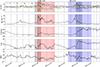 |
Figure 1 Solar wind in-situ observation from the OMNI dataset that contain both an ICME and a SIR. From top to bottom are represented the Interplanetary Magnetic Field amplitude and components in Geospheric Solar Magnetospheric (GSM) coordinates, the proton number density, the solar wind velocity, the proton temperature and the plasma parameter β. The vertical solid gray lines indicate the cells on which the identification is made. The ICME (resp. SIR) from the reference catalog is indicated between the red (resp. blue) dashed lines. The grey shaded intervals represent the cells that are responsible for the detection of the ICME (resp. the SIR) represented by the red (resp. blue) interval, the associated vertical solid line that represents their associated characteristic time and the confidence score with which those events are identified, as detailed in Section 2. |
It is worth noting here that a measuring spacecraft will see those signatures when going through those interplanetary events. It will thus only be able to observe them through a one-dimensional slice which cannot account for their entire spatial structure. As a consequence, there is a strong variability in the in-situ signature of those events which include a strong variability in the definition of their starting and ending dates. The criteria mentioned above might then only be fulfilled partially or sparsely. The recognition of those in-situ signatures is made even more difficult with the existing cases of several events of different types that overlap one with another. This is for example the case for the 19–25 October 1999 event studied by Dal Lago et al. (2006).
For these reasons, identifying the in-situ signature of ICMEs and SIRs is ambiguous and time-consuming, and the resulting catalogs then necessarily diverge one from another. For instance, Chi et al. (2016) showed that on average, 80% of the ICMEs of a given list were considered in another one.
From then on, developing automated recognition scheme for both ICMEs and SIRs is a good solution to gain time and reduce the ambiguity of the task. To do so, several studies introduced thresholds based methods for the two types of events. This is for instance what was done by Lepping et al. (2005) and Ojeda-Gonzalez et al. (2017) for ICMEs and Grandin et al. (2019) for SIRs. However these threshold-based methods are inherently highly dependent on the considered dataset and cannot generalize to other events.
To leverage those constraints, some studies suggested relying on supervised learning techniques, and specifically deep learning-based methods. For instance, Nguyen et al. (2019) used an ensemble of convolutional neural networks (LeCun et al., 2010) to detect events by learning patterns from a synthetic multi-dimensional proxy array built from in-situ data. Following their work, Rüdisser et al. (2022) and Chen et al. (2022) used a Residual U-Net (ResUNet) (Jha et al., 2019) to detect events by the means of segmentation masks. It is also worth noting here the recent emergence of work made on the automatic recognition of in-situ flux rope signatures with machine learning (dos Santos et al., 2020; Narock et al., 2022; Farooki et al., 2024; Pal et al., 2024).
Coming back to the entire ICME start and end time estimation, the three first mentioned methods achieved similar detection performances that were above those obtained by the threshold-based methods. They also proved their ability to rapidly establish generic and reproducible event catalogs, with the ResUNet having the advantage of requiring less training time and post-processing. However these methods were trained using several pre-existing catalogs from the literature as their ground reference, and as such, their accuracy is limited by the ambiguity from these catalogs. Additionally, the raw outputs of these three methods were converted into an event catalogs after a certain number of post processing steps such as median filtering, peak detecion (Nguyen et al., 2019), removal of short events and merge of adjacent events (Chen et al., 2022; Rüdisser et al., 2022) that would be worth simplifying.
The three methods also have the advantage of requiring no physical apriori knowledge on the events they are detecting. This makes them easily adaptable from one type of events to another. Nevertheless, they were for now only tested on ICMEs. Their adaptation to SIRs have thus actually never been done. Moreover, they cannot account for overlapping events because of their intrinsic design. Additionally, although they could have been adapted from a mission to another, the dataset they rely on considered WIND specific features, such as proton fluxes, and thus making it much less straightforward. For instance, Rüdisser et al. (2022) had to remove a certain number of features from their dataset in order to apply their method on STEREO data. This is also why Pal et al. (2024) only considered the Interplanetary Magnetic Field when developing their pipeline.
Instead of relying on segmentation masks or on the construction of an artificial multi-dimensional proxy, another possibility is to directly identify time intervals that are likely to contain either an ICME or a SIR as represented by the red and blue intervals of Figure 1.
This approach is strongly inspired by the You Only Look Once (YOLO) family of algorithms in object detection. These methods, first introduced by Redmon et al. (2016), are particularly efficient when it comes to real-time object detection on video data. The basic idea behind YOLO stands in having a single neural network to encode an entire input sample (e.g. a frame in the case of a video) and directly predicting a bounding box likely to contain an object or a time interval in our case. This allows to properly consider the context around the objects to be detected while requiring almost no post-processing steps. As a consequence, these techniques have the advantage of providing fast visual indicators about event occurrences that could directly be interpreted by a human operator in an operational space weather context. Nowadays, YOLO type algorithms have widely been developed and applied in various field although this was never really done on time series data. We refer to Terven & Cordova-Esparza (2023) for an exhaustive review of the different evolutions of YOLO.
This paper presents a novel approach for the multi-class detection of interplanetary space weather events based on the YOLO principle applied to multivariate time-series data. Compared to the previous studies made on this topic, our method requiles less input data while rapidly providing straightforward visual indicators about an evento ccurrence without any additional post-processing steps. A specific statistical insight on the extended events catalog obtained with these methods would then consitute the topic of a future work. Section 2 focuses on data and event catalog, used by our pipeline which is detailed in Section 3. The pipeline’s identifications and mistakes are then evaluated and compared with other existing methods in Section 4.
2 Data
2.1 OMNI data
The previous attempts made on the automatic detection of ICMEs (Nguyen et al., 2019; Chen et al., 2022; Rüdisser et al., 2022) considered 33 different input variables derived from the WIND in-situ data measurements. Here, we decide using eight distinct features of the 1-min OMNI dataset between 1995 January 1 and 2024 June 30:
the three Geocentric Solar Magnetic (GSM) components of the IMF along with their amplitude, Bx, By, Bz, and B,
the proton number density, Np,
the proton temperature, T,
the bulk velocity, V,
the plasma parameter, β.
In addition to reducing the dimensionality of the input data, this simplifies future adaptation of our method to additional spacecraft data (for instance, this set of features is part of the one used by Rüdisser et al. (2022) when they applied their method on STEREO data).
Just like the previous attempts, we resample the data to a 10-minute resolution in order to remove as much data gaps as possible while still providing an accurate event identification. The data is normalized and scaled in order to have an average of 0 and a standard deviation of 1 for each feature.
The data is then grouped into 1024 datapoints long windows (which represents a little bit more than a week of data) that slides over the 1995–2024 period with a 6-hour stride. Finally, we remove the windows for which more than 10% of the data is missing, the remaining data holes being filled with linear interpolation. The dataset we are working with is then made of 37012 windows made of 1024 points each.
Naturally, the sliding windows length and stride as well as the proportion of missing data above which we discard the windows are adjustable parameters of our method. In this paper, we present parameters for which we obtained the best detection performances.
2.2 Event catalogs
In the introduction, we mentioned a certain number of existing ICME and SIR catalogs. This diversity comes from both the ambiguity one can have when observing in-situ data and the criteria used to define an event that differ from a catalog to another. In this work, we use the broadest definition of ICMEs and SIRs in order to be as exhaustive as possible. In the case of ICMEs, we use the criteria that are given in Chi et al. (2016). Concerning SIRs, we use the criteria that are used in Jian et al. (2006) and reminded in Allen et al. (2021). A given time interval is then considered as an ICME or a SIR if it fulfills at least three of the criteria that are summarized in Table 1. Additionally, as their existence usually lead to more geoeffective events (Kilpua et al., 2017a; Chi et al., 2018), and given the operational application of our work, we consider in this paper the sheath and HSS region (whenever they exist) to be part of ICME-driven and SIR-driven events, respectively.
Criteria used to define ICMEs and SIRs.
For exhaustivity purposes, the so-called reference catalogs we use in this paper primarily consist of an aggregate of existing ICME and SIR catalogs. In the case of ICME, we gather the lists of Nguyen et al. (2019), Möstl et al. (2017), Richardson & Cane (2010), and Nieves-Chinchilla et al. (2018). Concerning the SIRs, we combine the catalog presented in Chi et al. (2018) to events detected with the method presented in Grandin et al. (2019) on OMNI data between 1995 and 2024. As some of those catalogs were established with either WIND or ACE in-situ data measurements, the events beginning and ending times could slightly differ from their actual one in OMNI data. Those differences were manually corrected following the criteria listed in Table 1. The same correction was made when an event was found to be present in several catalogs. Finally, during the various tests made on our method, additional ICMEs and SIRs that were not present in any list were manually identified following the criteria listed in Table 1 and progressively added to our catalog. Additional detail about the different catalogs we use in this study can be found in Table 2. It is worth mentioning here that each time new events were found, they have been added to our catalog and the neural network has been retrained from scratch.
Details about the aggregated ICMEs and SIRs catalogs.
We finally kept the events for which we have available data windows as defined in the previous subsection. The ICMEs and SIRs catalogs we use to develop our method are then made of 840 ICMEs, 60 of which being newly identified events, and 1237 SIRs, 140 of which being newly identified events. Because the two type of events can overlap one with another, the two catalogs are not completely disjoint. In fact, 282 ICMEs overlap events from the SIRs catalog for more than 10% of their duration and 239 SIRs overlap events from the ICMEs catalog for more than 10% of their duration. It is worth noting here that those overlap rates are enhanced by the consideration of the sheath and the HSS region whenever they exist as they necessarily lead to larger events.
As mentioned in Nguyen et al. (2019), we do not expect those so-called reference catalogs to be completely exhaustive. They are still among the most exhaustive ones and are intended to be automatically updated with the method presented in this paper.1
3 Method
In this section, we present the global and detailed principles of the model, namely SPODIfY (Space Plasma Object Detection Inspired from YOLO), that we develop to provide a multi-class detection of ICMEs and SIRs. First, we present the global detection strategy along with the dataset labels. Then, we present the neural network architecture used for SPODIfY and its training procedure. Finally, we detail the evaluation benchmarks.
As a general preliminary remark, our work is not a straightforward application of an existing YOLO algorithm to our dataset. It is instead an approach inspired by these techniques. An exhaustive comparison of our method with the different existing YOLO type algorithms can be found in Appendix A. In addition to the application of our method on text book cases as in Figure 1, we show additional, less obvious identification examples along with errors made by our method in Appendix B.
3.1 Time interval definition
For a given window of data X that has a duration wX (here corresponding to 1024 data points), SPODIfY reasons globally about the entire window, including all the objects it possibly contains and identifies time intervals that are likely to contain an ICME or a SIR. It is already worth noting here that, instead of having each identified interval capable of detecting every type of object, we rather identify one interval per type of object we wish to detect. This major difference with object detection is made to account for the possible superposition of solar wind transient events and allows an external user of SPODIfY to leverage this possible amibiguity by themselves.
The data window X is divided into Ncells elements or cells that are typically delimited by the vertical gray solid lines in Figure 1. When a characteristic time of an object falls within a cell, the latter is responsible of detecting this object. This is for instance what happens for the two gray colored cells of Figure 1 that are responsible for the detection of an ICME and a SIR respectively. The so-called characteristic time corresponds to events start dates for ICMEs and center dates for SIRs and are represented in Figure 1 by the vertical solid red and blue lines respectively.
In this paper, we set Ncells = 16, which is equivalent to setting the duration of each cell to Δt = 640 min. Intrinsically, YOLO type algorithms are known for their inability to distinguish objects that fall within the same cell (Terven & Cordova-Esparza, 2023, and references therein). Consequently, with such value of Ncells we will not be able to distinguish two ICMEs or two SIRs which characteristic times are less than 640 min one from each other. As this only concerns a single ICME and a single SIR from the reference catalogs, this choice will not affect the SPODIfY performances significantly.
For each cell j that starts at tj, SPODIfY identifies one time interval or possible event per object class that are considered. Such possible events are typically represented by the red and blue shaded intervals in Figure 1. In this paper, we aim to detect ICMEs and SIRs as defined in the previous section. We thus consider here Nobjects = 2 object classes. Each time interval Eij, i corresponding to a given object class, is defined by two values: the relative position within the cell of its characteristic date tij and its duration relative to the window duration wij. In our case, this characteristic date corresponds to the beginning date for ICMEs and the center date for SIRs as represented by the red and blue vertical lines in Figure 1. Eij also comes with a confidence score pij of belonging to a particular class of object as represented in the top panel of Figure 1. The output of SPODIfY is then a three-dimensional tensor of size (Nobjects × Ncells × 3). The possible multiple detections are removed through non-maximal suppression based on the intersection over union of the concerned identified events. The final events identified by SPODIfY can then be filtered through a threshold set on their associated confidence score.
We illustrate how SPODIfY deals with overlapping events in Figure B1 for the 19–25 October 1999 event described in Dal Lago et al. (2006). The two overlapping ICME and SIR delimited by the dashed line are both detected and the identified events also overlap one with another. In comparison with the reference SIR, SPODIfY identifies a SIR extended to the high velocity region downstream the ICME. This could thus still be considered a consistent identification regarding the general physical properties of SIRs. We will come back on this statement in Section 4.3.
3.2 Labeling
During the training phase, we define the labels tij, wij, and pij as being equal to 0 except if a reference event Eij has its characteristic date tE in the cell j. In this case, tij, wij, and pij are defined as follows:
 (1)
(1)
 (2)
(2)
 (3)
(3)
where wE is the duration of Ei and  the duration of its temporal overlap with the window X. Given the choice made for their duration, a cell can overlap with several events belonging to the same class at the same time. Although scarce, we define in this case the labels with regards to the largest of the concerned events.
3.3 Model architecture
SPODIfY architecture consists of a simple Convolutional Neural Network with an encoder-decoder structure. The encoder, in charge of extracting useful features for object detection from the data, is made of five convolutional layers, an ensemble of convolutional filters that convolve with the input data in order to extract the most useful features. The output of each layer is rescaled and re-centered into a zero mean and a unit variance by an operation called batch normalization (BN) (Ioffe & Szegedy, 2015). The dimensionality is then reduced with an operation called Max Pooling that extracts the maximal values on output patches.
The decoder, in charge of converting the features extracted by the encoder in actual bounding boxes, is made of two fully connected (FC) or linear layers. A complete description of SPODIfY architecture is found in Table 3.
SPODIfY architecture.
The output of each layer is activated with a Leaky Rectified Linear Unit activation function, defined as ϕ(x) = x if x > 0 and 0.1x otherwise, except for the final layer that is activated by a sigmoid function defined as  .
.
3.4 Training
SPODIfY was implemented within the Pytorch framework (Paszke et al., 2019) for Python. We optimize the model weights with a Stochastic Gradient Descent (SGD) that we select over other existing optimizers for its enhanced generalization capacity (Hardt et al., 2016). The model is trained for 100 epochs with a learning rate scheduled as follows: for the first 10 epochs, the learning rate gradually increases from 10−4 to 10−3. The model is then trained at 10−3 for 5 epochs then 10−4 for 5 additional epochs and 10−5 until training ends.
Training consists in minimizing the following multi-part loss function:
 (4)
(4)
where  is the event that belongs to the class i identified in the jth cell and
  is the associated confidence score estimated by SPODIfY. δij = 1 if the jth cell contains a reference event Eij that belongs to the class i, 0 otherwise.
The first two terms in equation (4) directly account for the error made by our model while identifying intervals in cells that actually contain the characteristic time of an event. In order to emphasize on event identification, those two terms are weighted with the two parameters λbox and λobj that are both set equal to 5, as done in Redmon et al. (2016). The last term in equati(4)on accounts for the error made by SPODIfY while estimating the confidence score in the cells that do not contain objects belonging to the class i. In order to give more importance to the cells that actually contain objects, we set its associated weight λnoobj = 0.5, as done in Redmon et al. (2016).
The Generalized Intersection over Union (GIoU) is a differentiable extension of the temporal Intersection over Union (IoU) of two events that can be expressed as:
 (5)
(5)
where C is the smallest event that contains both Eij and  .
.
In order to evaluate our model on the entire dataset, we use nested cross-validation as done in Bernoux et al. (2022). The dataset is split into yearly folds and the test set will vary across the data one fold at a time. The remaining folds being grouped into three 9 years long two 9 years long, and one 10 years long batches on which we run a cross-validation scheme resulting in the total training of 3 × 29 = 87 models. The predictions made on the test sets are then averaged in order to obtain a single prediction on the entire dataset period.
We use a batch size of 32 and the training examples are shuffled after each epoch. On Nvidia Quadro RTX 6000, a single model is trained in 50 min. Naturally, the optimizer, the number of epochs, our sheduling strategy and the values of the weights λbox, λobj, and λnoobj are all tunable hyperparameters of our model. Although various tests have been attempted, the set of hyperparameters chosen in this paper are the one for which we obtained the best detection performances on the validation set.
3.5 Baseline
For benchmark purposes, we adapted one of the existing ResUNet architecture (Chen et al., 2022; Rüdisser et al., 2022) to the simultaneous detection of ICMEs and SIRs. Just like SPODIfY, this is done through the prediction of one segmentation mask per type of event, this to take into account the possibility of overlapping events. As the two existing methods offer little architecture difference while reaching similar overall detection performance, it was no use adapting both and we thus decided to retain the architecture introduced by Rüdisser et al. (2022). In the following, this baseline will be designated as ResUNet++.
In addition to ResUnet++, we also compare SPODIfY with threshold-based methods previously introduced in past studies.
For ICMEs, we define the following criteria inspired by the one introduced in Lepping et al. (2005):
 (6)
(6)
 (7)
(7)
 (8)
(8)
and consider any interval respecting those criteria for more than 2 hours to be a detected ICME.
For SIRs, we select the method presented in Grandin et al. (2019) that relies on empirical thresholds set on the solar wind velocity and the IMF amplitude variations. We refer to the aforementioned publication for a complete descritpion of this method.
The two threshold-based methods we are using were introduced to detect ICMEs and SIRs with the most obvious in-situ signature. For instance, Lepping et al. (2005) primarily deals with magnetic clouds, the subset of ICME that respects all of the criteria listed in Table 1, and Grandin et al. (2019) primarily deals with SIRs that are followed by a HSS region. We thus expect those method to make little detection mistakes while missing an important number of events.
3.6 Model evaluation
As the aim of SPODIfY is to provide a straightforward identification of events beginning and ending times, we evaluate its detection performances from an event-based perspective. To do so, we generate event catalogs by applying a global non-maximal suppression algorithm to the identifications made in all of our dataset windows. The generated catalogs are then filtered according to a certin confidence score threshold that can be different for each event type and compared to the reference catalogs introduced in Section 2.2:
An event E from a reference catalog is called detected if it is overlapped by at least one of the events identified by a model. Otherwise it is called a False Negative (FN)
An identified event
 is called a True Positive (TP) if it overlaps an event from the associated reference catalog. Otherwise it is called a False Positive (FP).
With these definitions, we define for each event type a recall  , a precision
  and a F1-score
  that serve as evaluation metrics.
In addition, we evaluate the errors made on the beginning and ending times of an event E of duration wE, detected by an event  , by the Percentage Error (PE) and the Absolute Percentage Error (APE) defined as follows:
 (9)
(9)
 (10)
(10)
where τ denotes the event beginning or ending times. With this convention, a positive PE indicates that  begins or ends earlier than E.
The choice of a percentage error over a temporal error was made to account for the high duration variability we have in the reference catalogs (between 2 h 43 min and 110 h 7 min for ICMEs and between 5 h 26 min and 11 d 23 h for SIR/HSS). With this choice, a 10 h prediction delay is for instance more impacting for a 10 h event than for a 50 h event on an overall model detection performance. In Section 4.3, we will be considering the PE and APE distribution over all of the events identified by SPODIfY and the different baseline methods.
We remind here that both the ICME and the SIR reference catalogs, as any other existing catalogs are not exhaustive and include strong variabilities in the definition of the events starting and ending dates. Consequently, the labels do not represent an absolute truth. The performance metrics presented in this section only indicate how similar the event lists generated by our model are to the reference catalogs. We thus do not expect those metrics to be perfect.
4 Results
4.1 Precisions and recalls evaluation
For each event type, we compute SPODIfY and ResUNet++ precision and recall for varying confidence score thresholds.2 We represent those evolutions in Figure 2. Both the solid and the dashed precision-recall curves exhibit very similar evolutions with the solid ones being slightly above the dashed ones, especially in the SIR case. This indicates that SPODIfY slightly outperforms ResUNet++ in terms of event-based SIR detection with maximal recall and precision values that are never reached by ResUNet++. This statement is particularly true for the working points indicated by the red and blue dots in the two panels that correspond to the maximal value reached by the F1 score. It also means that SPODIfY and ResUNet++ achieve similar performances in terms of event-based ICME detection. It is worth mentioning here that the results shown for ResUNet++ are those obtained after removing the identified events with a duration below 2 hr as done in Rüdisser et al. (2022) while SPODIfY results are directly evaluated on the algorithm raw output. Removing this filtering step on ResUNet++ would have led to even lower precisions and recalls. For every method we tested, the F1 scores are higher for the SIRs. This is not surprising as their typical in-situ signature is simpler to define than the one we have for ICMEs.
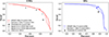 |
Figure 2 Precision-Recall curve of SPODIfY (solid lines) and ResUNet++ (dashed lines) for ICME (red, left) and SIR (blue, right) detection. The dots indicate the maximal F1-score reached by the two models for each event type and the black markers on both panel indicate the recalls and precisions obtained by the threshold-based methods, Nguyen et al. (2019) and Chen et al. (2022). |
For both ICMEs and SIRs, the precision of threshold-based methods is comparable to the one reached by SPODIfY and ResUNet++ with a much lower recall. This result was expected for the reasons mentioned in Section 3.5 and thus shows that SPODIfY and ResUnet++ clearly outperform the threshold-based methods. Although not exactly comparable, we also indicated the detection performances mentioned in Nguyen et al. (2019) and Chen et al. (2022). As those scores are below SPODIfY precision-recall curve, one can also infer our model to overcome those two other methods.
As mentioned previously, the detection performances will be limited by the ambiguity of the existing event catalogs. We thus do not expect those detection scores to be higher than the average similarity found between two catalogs manually-made on the same dataset by different observers. In the case of ICMEs, Chi et al. (2016) estimated this similarity to be around 80% which is very close to the maximal F1 score reached by SPODIfY. From a pure precision and recall perspective, the lists generated by our model are then comparable to those manually made by human observers. Consequently, future efforts made on the automatic detection of ICMEs should focus on the other detection aspects that will be depicted later-on rather than the sole question of having an event detected.
4.2 Insight on the false positives and false negatives
We complete the evaluation done in the previous section with a statistical insight on the errors made by our model. We remind here that the False Positives and the False Negatives we are studying in this section are defined with regards to the reference catalogs. They then might not always be considered as errors made by our model. This being said, we select the working point indicated by the colored dot in Figure 2. At those working points corresponding to the F1 scores indicated in Figure 2, SPODIfY detects 644 out of 840 ICMEs and 1110 out of 1237 SIRs for a recall being equal to 0.767 and 0.897, respectively. 702 of the 876 identified ICMEs and 1166 of the 1358 identified SIRs are considered as TPs for a precision being equal to 0.801 and 0.859, respectively. Although surprising, the difference noticed in the number of identified and reference events are understandable as an identified event can detect several reference event and reciprocally.
Figure 3a presents the median value of the plasma β as a function of the maximal IMF amplitude Bmax for each ICME in the reference catalog. Obviously, the demarcation between detected events, in green, and FNs, in orange, is not perfectly clear, threshold-based methods would have performed perfectly otherwise.
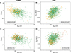 |
Figure 3 Left column: median value of the plasma β as a function of the maximal IMF amplitude Bmax for the ICMEs in the reference catalog (a) and those identified by SPODIfY (c). Right column: maximal value of the plasma bulk velocity Vmax as a function of the maximal IMF amplitude Bmax for the SIRs in the reference catalog (b) and those identified by SPODIfY (d). The green dots in the top (resp. bottom) panel represent the events detected by SPODIfY (resp. the TPs). The orange in the top (resp. bottom) panel represent the FNs (resp. the FPs). In the bottom panel, the orange dots circled in red indicate the misclassified events. |
Nevertheless, one can still notice that the great majority of the FNs are located in the upper left part of the panel thus corresponding to the weakest IMF amplitudes and the highest β values. We then expect the FNs to be the events which in-situ signature differs the most with the expected typical in-situ signature of ICMEs as detailed in the introduction. This is typically the case for the event shown in Figure B2 where the IMF amplitude hardly goes above 5 nT, β goes punctually above 1 and the bulk velocity goes below 400 km/s. From an operational perspective, those events are also expected to among the least geoeffective. Missing them is thus less impacting as long as the most prominent events are correctly detected, which is the case for the quasi-totality of the events located in the bottom right corner. The only exception actually corresponds to October 2003 Halloween storm for which the amount of missing data within the event was too large to provide a meaningful identification.
We show the same representation for the identified ICMEs in Figure 3c. Here again, the TPs, in green, are hardly distinguishable from the FPs, in orange, indicating that the identification errors made by our model are events that already exhibit part of the expected typical in-situ ICME signature. Just like the FNs, the great majority of FPs are located on the panel upper left corner. They are then among the less prominent identified events, thus expected to be the least geoeffective. This is also the case for the event shown in Figure B4 where the detected event presents a low β value that regularly goes above 1, an enhanced velocity with declining profile and a rotating IMF with a weak amplitude hardly distinguishable from the surrounding ambient solar wind.
It is also worth noting that the TPs and the detected ICMEs have similar distributions in this plane. This indicates the physical consistency of the events list generated by SPODIfY.
The same conclusions can be drawn for SIRs as represented in the right column of Figure 3. In this case, we represent the maximal value of the solar wind bulk velocity Vmax instead of the median value of β. This representation once again shows that most of the FPs and FNs are in the bottom left corner of their respective panel and thus are the events which in-situ signature differs the most from the expected SIR typical in-situ signature. Typical examples of such FNs and FPs are represented in Figures B3 and B5. We also here have both TPs and detected SIRs exhibiting similar distributions indicating the global physical consistency of the SIR list generated by SPODIfY.
The identification errors made by SPODIfY then correspond to questionable events that exhibit a weak and questionable in-situ signature in comparison to the typical expected one.This statement is reinforced by the kernel density estimates of the events duration represented in Figure 4. For both ICMEs (Fig. 4, left column) and SIRs (Fig. 4, right column), FNs (Figs. 4a and 4b), and FPs (Figs. 4c and 4d) are on average shorter than the actual detected events or TPs (solid green lines) and are thus even more questionable regarding their actual belonging to either the reference of the identified catalogs. It is also worth pointing out here that the largest SIRs identified by our model have a maximal duration of 6 d 22 h 37 min and is thus shorter than the largest SIRs of our reference duration that lasts up to 11 d 23 h. This comes from the choice we made in the window size that is shorter than the maximal SIR duration found in the reference catalog. Those findings extend the conclusions previously drawn in the past results of Nguyen et al. (2019) and Chen et al. (2022) to the SIR case and keep indicating how ambiguous it is to recognize an event in-situ signature.
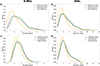 |
Figure 4 Left (resp. right) column: kernel density estimates of the ICMEs durations (resp. SIRs) in the reference catalog (top panel) and those identified by SPODIfY (bottom panel). On the top (resp. bottom) panels, the black curves refer to the entire reference catalog (resp. the entire identified catalog), the green curves refer to the detected events (resp. the TPs) and the orange curves refer to the FNs (resp. FPs). |
Coming back at Figure 3, quasi-totality of the FPs that exhibit the most prominent in-situ signatures, e.g., those that have an enhanced maximal IMF amplitude Bmax are actually real events from the other class reference catalog. At the working point we consider, those events, circled in red in Figure 3 represent 54% of the ICMEs falsely identified (94 events out of 174) and 44.8% of the SIRs falsely identified (86 events out of 192). Ratio that goes up to 68.7% (79 events out of 115) and 58.7% (74 events out of 126) respectively if we just consider the FPs with the highest IMF amplitude i.e. those for which Bmax > 10 nT.
In a pure mono-class paradigm, such a confusion is perfectible and future work could be oriented toward an improvement of the inner-class distinction. Nevertheless, the ratio of identified events that overlap the identified events from the other class for more than 10% of their total duration (30.4% of the identified ICMEs and 25.4% of the SIRs by counting both TPS and FPs) is comparable to the ratio of event belonging to both classes as described in Section 2.2. Our model then only reflects the ambiguity that exists when an external, human, observer distinguishes an ICME from an SIR. As shown in Nguyen et al. (2019), we are once again limited by the ambiguity of the reference catalogs at the core of the supervised training.
This limitation will always be a bottleneck of multi-class automatic detection of solar wind events with supervised learning, misclassifying events while still detecting them could actually be an asset from an operational perspective. Indeed, detecting an event without determining its type is already useful information in order to estimate their possible geoeffective consequences. In fact, considering an overall detection metrics instead of a metrics per event type would have lead to a global maximal F1-score of 0.903 with the events with the most prominent in-situ signature being systematically detected. This makes our model already suitable for an operational usage.
4.3 Errors made on the events beginning and ending times
Having evaluated the detection performances of our model, we now investigate its capacity to accurately estimate the event beginning and ending times. The PE and APE distribution we obtain for SPODIfY and the baseline models and for the two event types are shown in Figure 5.
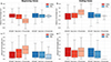 |
Figure 5 Box plots for the relative (a and b) and absolute (c and d) percentage error made on the beginning times (a and c) and ending times (b and d) made by SPODIfY, ResUnet++ and the threshold-based methods on their respective detected ICMEs (red boxes) and SIRs (blue boxes). The boxes are displayed between the 25th and the 75th percentiles and the whiskers between the 5th and 95th percentiles. For each box, the solid black line indicate the median while the black dashed line indicate the mean. |
Looking at the red boxes in Figures 5a and 5b, we first notice an almost unbiased estimation of ICMEs beginning times by SPODIfY that must be compared to the slightly late biased estimation offered by ResUNet++. On the opposite, ResUNet++ provides an almost unbiased estimation of ICMEs ending times while SPODIfY tends to estimate them slightly later than what was identified in the reference catalog. Combined altogether, these boxes indicate that SPODIfY and ResUnet++ identifies ICMEs with similar duration distributions with little discrepancies in the determination of the event beginning and ending times, the former being at the advantage of SPODIfY, the latter being at the advantage of ResUnet++. By comparison, thresholds provide a late biased estimation of ICMEs beginning time along with a nearly-biased estimation of their ending times, resulting in much shorter identified ICMEs in comparison to the ground truth. This ends up showing the efficiency of deep-learning based methods over thresholds for the automatic ICME detection task.
The statements we just made about ICME identification are confirmed by the APE distribution shown by the red boxes of Figures 5c and 5d. However, these metrics must be cautiously interpreted. Indeed, past studies revealed how ambiguous is the accurate determination of ICMEs beginning and ending time (Chi et al., 2016; Kilpua et al., 2017a; Nguyen et al., 2019, and references therein). Determining the ending time is particularly uncertain as it often corresponds to a smooth return to the surrounding ambient solar wind. This explains why we have increased error metrics on the ICMEs ending times. Consequently, the boxes shown in Figure 5 must be interpreted with regards to the reference catalogs that were used to train the detection algorithm. In fact and after visual inspection, 82 of the 644 ICMEs detected with SPODIfY (12.7%) were identified with a consistent ending time regarding the expected typical in-situ ICME signature. This is typically the case for the event shown in Figure B6 where although identified later than the reference event, the ending time extends to the region of enhanced IMF and low plasma β. This is also the case for the event shown in Figure B7 where the predicted ICME covers two successive events. A similar statement could also be made on SIRs, as illustrated in Figure B1 where the identified event actually extends to the high velocity region, not retained by the threshold-based method of Grandin et al. (2019) because of the overlap with the ICME.
In the SIR case, the blue boxes in Figures 5a and 5b indicate that both SPODifY and ResUNet++ estimate the beginning times with a slight early bias, resulting in events slightly shifted to the left on a time axis with respect to the reference catalog. On this point, ResUnet++ performs slightly better, as its percentage error distribution are almost unbiased for both beginning and ending times. This difference is however small and the narrower APE distributions shown by the blue boxes of Figures 5c and 5d actually suggests that, in a similar manner than in the ICME case, SPODIfY (resp. ResUNet++) performs slightly better at estimating the SIRs beginning (resp. ending) times. This results in the two methods identifying SIRs with similar duration distributions and little discrepancies between the events beginning and ending times.
At first sight, SPODIfY performs better on some points while ResUNet++ performs better on others. Those metrics must however be interpreted carefully as they only reflect the capacity of the two methods to reproduce the events beginning and ending times as defined in the reference catalogs that are uncertain. Additionally, those metrics come with high error bars that reflects the variability of the event characteristic times both in the reference and in the identified catalogs. With such variability, the detection performances of both SPODIfY and ResUNet++ can thus be considered as comparable if not mostly similar.
In the SIR case, threshold-based methods result in very narrow boxes as shown in the four panels of Figure 5, the high mean observed in Figure 5d being due to sparse distribution outliers not shown in Figure 5. This is easily understandable as part of the SIR reference catalog has been elaborated using this threshold-based method. The difference with deep-learning based methods then stands in the SIRs that are not followed by a significant HSS region but are still detected by SPODIfY and ResUnet++, as shown with the precisions and recalls shown in Figure 2. From then on, an interesting compromise solution to enhance the automatic generation of SIR catalog would be to first pre-select the SIRs intervals with either SPODIfY or ResUNet++ and then refine the events beginning and ending times with the thresholds, which would allow to benefit from the advantages of the two methods.
We now give an insight on the largest errors made by SPODIfY on the event beginning and ending times. Figure 6 represents the percentage error obtained for each detected events (ICMEs on the left column, SIRs on the right column) as a function of their duration and colored by their associated confidence score.
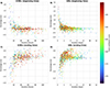 |
Figure 6 Percentage errors on the beginning times (upper row) and ending times (bottom row) of the ICMEs (left column) and the SIRs (right column) detected by SPODIfY as a function of their duration. The colorscale indicate the confidence score with which each event is identified. |
At first, we notice that the majority of the ICME beginning times, on Figure 6a, are estimated with a PE being close to 0. This is particularly true for those that are identified with the highest confidence scores. On the opposite, the ICMEs for which beginning times are estimated with the highest errors are mostly located on the upper left part of Figure 6a. They correspond to the shortest events of the reference catalogs and, whatsmore, they are mainly identified with the lowest confidence scores. Additionally, a visual inspection evidenced the two events identified with PEs below −0.5 to be long during flux ropes with a weak IMF amplitude in comparison to the surrounding ambient solar wind. We thus expect the events identified with the highest PE over their beginning time to be among those with the most ambiguous in-situ signature and consequently the one expected to be among the less geoeffective.
We observe the same behavior for SIRs beginning times, on Figure 6b, with an enhanced variability, already illustrated in Figure 5, that comes from the fact SIR beginning times are less clearly defined than those of ICMEs. Although noisier, the same statements apply for both ICMEs and SIRs ending times (on Figs. 6c and 6d) with the notable difference of the percentage error being mainly negative as this was suggested by the PE distribution shown in Figure 5.
Finally, the SIRs with the longest durations (above 7.5 days) are detected with the lowest confidence scores. Just like the overall shortest durations observed in Figure 4, this comes from the choice we made on our window size. Naturally, one could think increasing it would then probably allow detecting those events with enhanced confidence score and more consistent durations. Nevertheless, the attempt we made accordingly lead to reduced overall detection performances.
5 Conclusions and perspectives
In this paper, we focused on the automatic detection of ICMEs and SIRs in streaming, in-situ solar wind monitor data. Our approach, namely SPODIfY is inspired by the YOLO family of algorithms and consists in identifying time intervals for each type of events with a single convolutional neural network and no post-processing steps but non-maximal suppression to avoid event superposition.
This approach provides a fast visual indicator about the presence of ICMEs and/or SIRs in a given window of data and could thus easily be implemented in data visualization tools. From a pure scientific perspective such indicators are a key asset in the precise establishment and extension of interplanetary space weather events catalogs. Indeed, such method allows to already preselect the intervals of interest. An observer would then just have to properly adjust the beginning and ending times to their own requirements and/or criteria, possibly through the utilization of threshold-based methods. Those indicators can also be used, in an operational framework, to define ICMEs or a SIRs based space weather scenarii or to give clues about what possibly happened when onboard anomalies have been detected by spacecraft operators. For now, it allowed the extension of existing ICMEs and SIRs catalogs until mid-2024 and definitely appeal, as a future work, for deeper statistical insight into the physical properties of the two events types.
Because it requires no particular physical knowledge about ICMEs nor SIRs, our method could also be extended to additional event types. For instance, we could think about separating ICMEs from their possible sheath or adding a particular class for Magnetic Clouds, the subset of ICMEs having the most prominent in-situ signatures and expected to be the most geoeffective events.
In comparison with past attempts, our approach only requires eight input features common to a great number of spacecrafts measuring both the IMF and solar wind physical parameters (ACE, WIND, STEREO, DSCOVR, Solar Orbiter, Parker Solar Probe, etc.). It is then quite easy to adapt it from a spacecraft to another without generalization loss as this could be the case in the pipelines presented in Nguyen et al. (2019), Chen et al. (2022), and Rüdisser et al. (2022). As a proof of concept, Figure B7 shows an identification on DSCOVR during the May 11th 2024 event made by the model presented in this paper without any cross-calibration consideration. The undoubtful event detection and its classification as an ICME with an almost perfect beginning time estimation paves the way for future adaptation of our pipeline.
On the one hand, and despite of a much simpler and more straightforward architecture, SPODIfY detection performances are slightly better than those of other existing methods based on more complex neural network design and additional post-processing steps. In the wake of what was shown in past studies, those performances have been found limited by the intrinsic ambiguity that exists in the reference catalogs used for the supervised training. These limitations have been exhibited in a mono-class paradigm with detection errors corresponding to short events with the least prominent in-situ signatures. They have also been exhibited in a multi-class paradigm with a non-negligible part of the identified False Positives of a given class actually corresponding to events from the other class.
On the other hand, the error made by SPODIfY when estimating events beginning and ending times has been found to be comparable to the one made by existing past methods. Those dates are however still estimated with an important variability. Consequently, future work made on the subject should rather focus on improving the determination of those characteristic times rather than trying to improve the event-based detection performance significantly. A straightforward option could be to reduce the data temporal resolution, as enhanced detection performances were exhibited by Chen et al. (2022) when doing so.
As shown in Figure B7 our pipeline appears to be easily adaptable to another spacecraft. We could then also think about increasing the dataset size by considering a multi-spacecraft training. Dataset that could also be increased through the synthetic generation of solar events, by data augmentation techniques or by more advanced deep learning techniques such as Conditional Variational Autoencoders (Zhang et al., 2021).
Finally, a more operational way to evaluate our model performance would have stood in evaluating its early-detection capacity. Nevertheless, the label defined in this paper and on which the entire training relies on has been defined with the overlap between a given event and a given window of data. In an ideal case, SPODIfY will then start providing detections with significant confidence score once an important part of the event is already in the window i.e. when already begun for several hours if not days. Consequently, and although not tested in this paper, we expect poor early-detection performances of our method as is. It would then be really interesting to investigate the efficiency of techniques more adapted to time-series early detection on such task and future attempts should focus on this operational objective.
Acknowledgments
The authors thank ONERA/DPHY/ERS team, Nicolas Aunai, Hannah Rüdisser and Maxime Grandin for relevant and fruitful discussions. The OMNI data were obtained from the GSFC/SPDF OMNIWeb interface at the website (http://omniweb.gsfc.nasa.gov). The authors thank the DSCOVR and the CDPP AMDA team for the open-access data used in this study. The research leading to these results is part of ONERA Forecasting Ionosphere and Radiation belts Short Time Scale disturbances with extended horizon (FIRSTS) internal project. The editor thanks two anonymous reviewers for their assistance in evaluating this paper.
Appendix A: Similarities and differences with the YOLO type algorithms
The clearest differences between our model and YOLO type algorithms stand in the predicted bounding boxes. SPODIfY outputs are monodimensional and defined by three parameters while YOLO are bi-dimensional and defined by five parameters. This is because of the intrinsic nature of our input data. Additionnally, the boxes predicted by YOLO type algorithms are associated with a probability score for each of the classes they have been trained to detect. On the contrary, SPODIfY identifies one interval per class for the reasons that have been mentioned in Section 3.
Although adapted to our dataset specificities, SPODIfY has an architecture similar to the fast version of YOLOv1 introduced by Redmon et al. (2016). Apart from the number of convolutional layers and filters, the noticeable difference stand in the utilization of batch normalization instead of dropout as done since YOLOv2 (Redmon & Farhadi, 2017).
Finally, the choice of GIoU instead of a weighted Squared Error for the box term in equation (4) is similar to what has been done for YOLOv6 (Li et al., 2022).
Appendix B: Additional detection examples
In this appendix, we show additional ICMEs and SIRs identifications made by SPODIfY:
-
Figure B1 shows SPODIfY identification for the 19–25 October 2002 event described in Dal Lago et al. (2006) where an ICME and a SIR overlap.
Figure B2 represents an ICME False Negative.
-
Figure B3 represents a SIR False Negative.
-
Figure B4 represents an ICME False Positive.
Figure B5 represents a SIR False Positive.
-
Figure B6 represents an ICME for which SPODIfY estimates a consistent ending time.
Figure B7 shows a SPODIfY identification on DSCOVR solar wind observation during the May 11th 2024 event.
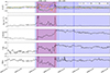 |
Figure B1 Solar wind in-situ observation from the OMNI dataset that contain overlapping ICME and SIR. The panels are the same as in Figure 1. |
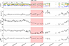 |
Figure B2 Solar wind in-situ observation from the OMNI dataset that contain an ICME False Negative. The panels are the same as in Figure 1. The ground truth is between the red dashed lines, the red interval represents the event identified by SPODIfY. |
 |
Figure B3 Solar wind in-situ observation from the OMNI dataset that contain a SIR False Negative. The panels are the same as in Figure 1. The ground truth is between the blue dashed lines, the blue interval represents the event identified by SPODIfY. |
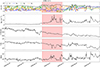 |
Figure B4 Solar wind in-situ observation from the OMNI dataset that contain an ICME False Positive. The panels are the same as in Figure 1. |
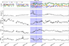 |
Figure B5 Solar wind in-situ observation from the OMNI dataset that contain a SIR False Positive. The panels are the same as in Figure 1. |
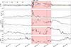 |
Figure B6 Solar wind in-situ observation from the OMNI dataset that contain an ICME for which SPODIfY estimates a consistent ending time. The panels are the same as in Figure 1. |
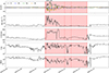 |
Figure B7 Solar wind in-situ observation provided by DSCOVR during the May 11th 2024 event. The panels are the same as in Figure 1. |
The ICME and the SIR reference catalogs can be accessed online at https://doi.org/10.57745/BYC2WC (Nguyen et al., 2025a).
Both ICMEs and SIRs catalogs obtained with SPODIfY can be accessed online at https://doi.org/10.57745/HDCAZ3 (Nguyen et al., 2025b).
References
- Allen RC, Ho GC, Jian LK, Vines SK, Bale SD, et al. 2021. A living catalog of stream interaction regions in the parker solar probe era. A&A 650: A25. https://doi.org/10.1051/0004-6361/202039833. [NASA ADS] [CrossRef] [EDP Sciences] [Google Scholar]
- Bernoux G, Brunet A, Buchlin É, Janvier M, Sicard A. 2022. Forecasting the geomagnetic activity several days in advance using neural networks driven by solar EUV imaging. J Geophys Res Space Phys 127(10): e2022JA030868. https://doi.org/10.1029/2022JA030868. [CrossRef] [Google Scholar]
- Chen J, Deng H, Li S, Li W, Chen H, Chen Y, Luo B. 2022. RU-net: a residual U-net for automatic interplanetary coronal mass ejection detection, Astrophys J Suppl Ser 259 (1): 8. https://doi.org/10.3847/1538-4365/ac4587. [CrossRef] [Google Scholar]
- Chi Y, Shen C, Luo B, Wang Y, Xu M. 2018. Geoeffectiveness of stream interaction regions from 1995 to 2016. Space Weather 16(12): 1960–1971. https://doi.org/10.1029/2018SW001894. [NASA ADS] [CrossRef] [Google Scholar]
- Chi Y, Shen C, Wang Y, Xu M, Ye P, Wang S. 2016. Statistical study of the interplanetary coronal mass ejections from 1995 to 2015. Solar Phys 291(8): 2419–2439. https://doi.org/10.1007/s11207-016-0971-5. [CrossRef] [Google Scholar]
- Dal Lago A, Gonzalez WD, Balmaceda LA, Vieira LEA, Echer E, et al. 2006 The 17–22 October (1999) solar-interplanetary-geomagnetic event: very intense geomagnetic storm associated with a pressure balance between interplanetary coronal mass ejection and a high-speed stream. J Geophys Res Space Phys 111(A7): A07S14. https://doi.org/10.1029/2005JA011394. [CrossRef] [Google Scholar]
- dos Santos LFG, Narock A, Nieves-Chinchilla T, Nuñez M, Kirk M. 2020. Identifying flux rope signatures using a deep neural network. Solar Phys 295(10): 131. https://doi.org/10.1007/s11207-020-01697-x. [CrossRef] [Google Scholar]
- Echer E, Tsurutani BT, Gonzalez WD. 2013. Interplanetary origins of moderate (−100 nT < Dst ≤ −50 nT) geomagnetic storms during solar cycle 23 (1996–2008). J Geophys Res Space Phys 118(1): 385–392. https://doi.org/10.1029/2012JA018086. [CrossRef] [Google Scholar]
- Farooki H, Abduallah Y, Noh SJ, Kim H, Bizos G, Shin Y, Wang JTL, Wang H. 2024. A machine learning approach to understanding the physical properties of magnetic flux ropes in the solar wind at 1 Au. Astrophys J 961(1): 81. https://doi.org/10.3847/1538-4357/ad0c52. [CrossRef] [Google Scholar]
- Gosling J, Pizzo V. 1999. Formation and evolution of corotating interaction regions and their three dimensional structure. Space Sci Rev 89(1): 21–52. https://doi.org/10.1023/A:1005291711900. [CrossRef] [Google Scholar]
- Gosling JT, Pizzo V, Bame SJ. 1973. Anomalously low proton temperatures in the solar wind following interplanetary shock waves – evidence for magnetic bottles? J Geophys Res 78(13): 2001–2009. https://doi.org/10.1029/JA078i013p02001. [CrossRef] [Google Scholar]
- Grandin M, Aikio AT, Kozlovsky A. 2019. Properties and geoeffectiveness of solar wind high-speed streams and stream interaction regions during solar cycles 23 and 24. J Geophys Res Space Phys 124(6): 3871–3892. https://doi.org/10.1029/2018JA026396. [CrossRef] [Google Scholar]
- Hardt M, Recht B, Singer Y. 2016. Train faster, generalize better: stability of stochastic gradient descent. https://doi.org/10.48550/arXiv.1509.01240 [cs. LG]. [Google Scholar]
- Ioffe S, Szegedy C. 2015. Batch normalization: accelerating deep network training by reducing internal covariate shift. Proc Mach Learn Res 37: 448–456. https://doi.org/10.48550/arXiv.1502.03167. [Google Scholar]
- Jha D, Smedsrud PH, Riegler MA, Johansen D, de Lange T, Halvorsen P, et al. 2019. ResUNet++: an advanced architecture for medical image segmentation. https://doi.org/10.48550/arXiv.1911.07067 [ecs, eess]. [Google Scholar]
- Jian L, Russell CT, Luhmann JG, Skoug RM. 2006. Properties of interplanetary coronal mass ejections at one au during 1995–2004. Solar Phys 239(1–2): 393–436. https://doi.org/10.1007/s11207-006-0133-2. [CrossRef] [Google Scholar]
- Kilpua EKJ, Balogh A, von Steiger R, Liu YD. 2017. Geoeffective properties of solar transients and stream interaction regions. Space Sci Rev 212(3): 1271–1314. https://doi.org/10.1007/s11214-017-0411-3. [Google Scholar]
- Kilpua EKJ, Koskinen HEJ, Pulkkinen TI. 2017. Coronal mass ejections and their sheath regions in interplanetary space. Living Rev Solar Phys 14(1): 5. https://doi.org/10.1007/s41116-017-0009-6. [CrossRef] [Google Scholar]
- LeCun Y, Kavukcuoglu K, Farabet C. 2010. Convolutional networks and applications in vision. In: Proceedings of 2010 IEEE International Symposium on Circuits and Systems, Paris, France, 30 May–2 June, IEEE, pp. 253–256. ISBN 978-1-4244-5308-5. https://doi.org/10.1109/ISCAS.2010.5537907. [Google Scholar]
- Lepping RP, Wu C-C, Berdichevsky DB. 2005. Automatic identification of magnetic clouds and cloud-like regions at 1 AU: occurrence rate and other properties. Ann Geophys 23(7): 2687–2704. https://doi.org/10.5194/angeo-23-2687-2005. [CrossRef] [Google Scholar]
- Li C, Li L, Jiang H, Weng K, Geng Y, et al. 2022. YOLOv6: a single stage object detection framework for industrial application. https://doi.org/10.48550/arXiv.2209.02976 [cs. CV]. [Google Scholar]
- Möstl C, Isavnin A, Boakes PD, Kilpua EKJ, Davies JA, et al. 2017. Modeling observations of solar coronal mass ejections with heliospheric imagers verified with the heliophysics system observatory. Space Weather 15(7): 955–970. https://doi.org/10.1002/2017SW001614. [CrossRef] [Google Scholar]
- Narock T, Narock A, Dos Santos LFG, Nieves-Chinchilla T. 2022. Identification of flux rope orientation via neural networks. Front Astron Space Sci 9: 838442. https://doi.org/10.3389/fspas.2022.838442. [CrossRef] [Google Scholar]
- Nguyen G, Aunai N, Fontaine D, Pennec EL, den Bossche JV, Jeandet A, Bakkali B, Vignoli L, Blancard BR-S. 2019. Automatic detection of interplanetary coronal mass ejections from in situ data: a deep learning approach. Astrophys J 874(2): 145. https://doi.org/10.3847/1538-4357/ab0d24. [CrossRef] [Google Scholar]
- Nguyen G, Bernoux G, Ferlin A. 2025a. Interplanetary solar events catalogs [Dataset]. Recherche Data Gouv. https://doi.org/10.57745/BYC2WC. [Google Scholar]
- Nguyen G, Bernoux G, Ferlin A. 2025b. Results of multi-class detection of solar events with a YOLO based approach. . Recherche Data Gouv. https://doi.org/10.57745/HDCAZ3. [Google Scholar]
- Nieves-Chinchilla T, Vourlidas A, Raymond JC, Linton MG, Al-haddad N, Savani NP, Szabo A, Hidalgo MA. 2018. Understanding the internal magnetic field configurations of icmes using more than 20 years of wind observations. Solar Phys 293(2): 25. https://doi.org/10.1007/s11207-018-1247-z. [CrossRef] [Google Scholar]
- Ojeda-Gonzalez A, Mendes O, Calzadilla A, Domingues MO, Prestes A, Klausner V. 2017. An alternative method for identifying interplanetary magnetic cloud regions. Astrophys J 837(2): 156. https://doi.org/10.3847/1538-4357/aa6034. [CrossRef] [Google Scholar]
- Pal S, dos Santos LFG, Weiss AJ, Narock T, Narock A, Nieves-Chinchilla T, Jian LK, Good SW. 2024. Automatic detection of large-scale flux ropes and their geoeffectiveness with a machine-learning approach. Astrophys J 972(1): 94. https://doi.org/10.3847/1538-4357/ad54c3. [CrossRef] [Google Scholar]
- Papitashvili NE, King JH. 2020. OMNI 1-min Data [Data set]. NASA Space Physics Data Facility. https://doi.org/10.48322/45bb-8792 (accessed on January 6, 2025). [Google Scholar]
- Paszke A, Gross S, Massa F, Lerer A, Bradbury J, et al. 2019. PyTorch: an imperative style, high-performance deep learning library. https://doi.org/10.48550/arXiv.1912.01703 [cs. LG]. [Google Scholar]
- Redmon J, Divvala S, Girshick R, Farhadi A. 2016. You only look once: unified, real-time object detection. In: 2016 IEEE Conference on Computer Vision and Pattern Recognition (CVPR), Las Vegas, NV, USA, 27–30 June, IEEE, pp. 779–788. https://doi.org/10.1109/CVPR.2016.91. [Google Scholar]
- Redmon J, Farhadi A. 2017. YOLO9000: better, faster, stronger. In: 2017 IEEE Conference on Computer Vision and Pattern Recognition (CVPR), Honolulu, HI, 21–26 July, IEEE, pp. 6517–6525. https://doi.org/10.1109/CVPR.2017.690. [Google Scholar]
- Richardson IG, Cane HV. 2010. Near-earth interplanetary coronal mass ejections during solar cycle 23 (1996–2009): catalog and summary of properties. Solar Phys 264(1): 189–237. https://doi.org/10.1007/s11207-010-9568-6. [CrossRef] [Google Scholar]
- Richardson, IG, Cane HV. 2012. Solar wind drivers of geomagnetic storms during more than four solar cycles. J Space Weather Space Clim 2: A01. https://doi.org/10.1051/swsc/2012001. [Google Scholar]
- Rüdisser HT, Windisch A, Amerstorfer UV, Möstl C, Amerstorfer T, Bailey RL, Reiss MA. 2022. Automatic detection of interplanetary coronal mass ejections in solar wind in situ data. Space Weather 20(10): e2022SW003149. https://doi.org/10.1029/2022SW003149. [CrossRef] [Google Scholar]
- Snyder CW, Neugebauer M, Rao UR. 1963. The solar wind velocity and its correlation with cosmic-ray variations and with solar and geomagnetic activity. J Geophys Res 68(24): 6361–6370. https://doi.org/10.1029/JZ068i024p06361. [CrossRef] [Google Scholar]
- Terven J, Cordova-Esparza D. 2023. A comprehensive review of YOLO architectures in computer vision: from YOLOv1 to YOLOv8 and YOLO-NAS. https://doi.org/10.48550/arXiv.2304.00501 [cs. CV]. [Google Scholar]
- Tsurutani BT, Gonzalez WD, Gonzalez ALC, Guarnieri FL, Gopalswamy N, et al. 2006. Corotating solar wind streams and recurrent geomagnetic activity: a review. J Geophys Res Space Phys 111(A7): A07S01. https://doi.org/10.1029/2005JA011273. [Google Scholar]
- Zhang C, Barbano R, Jin B. 2021. Conditional variational autoencoder for learned image reconstruction. https://doi.org/10.48550/arXiv.2110.1168 [cs. CV]. [Google Scholar]
Cite this article as: Nguyen G, Bernoux G & Ferlin A. 2025. Simultaneous multi-class detection of interplanetary space weather events. J. Space Weather Space Clim. 15, 21. https://doi.org/10.1051/swsc/2025016.
All Tables
All Figures
|
Figure 1 Solar wind in-situ observation from the OMNI dataset that contain both an ICME and a SIR. From top to bottom are represented the Interplanetary Magnetic Field amplitude and components in Geospheric Solar Magnetospheric (GSM) coordinates, the proton number density, the solar wind velocity, the proton temperature and the plasma parameter β. The vertical solid gray lines indicate the cells on which the identification is made. The ICME (resp. SIR) from the reference catalog is indicated between the red (resp. blue) dashed lines. The grey shaded intervals represent the cells that are responsible for the detection of the ICME (resp. the SIR) represented by the red (resp. blue) interval, the associated vertical solid line that represents their associated characteristic time and the confidence score with which those events are identified, as detailed in Section 2. |
| In the text | |
|
Figure 2 Precision-Recall curve of SPODIfY (solid lines) and ResUNet++ (dashed lines) for ICME (red, left) and SIR (blue, right) detection. The dots indicate the maximal F1-score reached by the two models for each event type and the black markers on both panel indicate the recalls and precisions obtained by the threshold-based methods, Nguyen et al. (2019) and Chen et al. (2022). |
| In the text | |
|
Figure 3 Left column: median value of the plasma β as a function of the maximal IMF amplitude Bmax for the ICMEs in the reference catalog (a) and those identified by SPODIfY (c). Right column: maximal value of the plasma bulk velocity Vmax as a function of the maximal IMF amplitude Bmax for the SIRs in the reference catalog (b) and those identified by SPODIfY (d). The green dots in the top (resp. bottom) panel represent the events detected by SPODIfY (resp. the TPs). The orange in the top (resp. bottom) panel represent the FNs (resp. the FPs). In the bottom panel, the orange dots circled in red indicate the misclassified events. |
| In the text | |
|
Figure 4 Left (resp. right) column: kernel density estimates of the ICMEs durations (resp. SIRs) in the reference catalog (top panel) and those identified by SPODIfY (bottom panel). On the top (resp. bottom) panels, the black curves refer to the entire reference catalog (resp. the entire identified catalog), the green curves refer to the detected events (resp. the TPs) and the orange curves refer to the FNs (resp. FPs). |
| In the text | |
|
Figure 5 Box plots for the relative (a and b) and absolute (c and d) percentage error made on the beginning times (a and c) and ending times (b and d) made by SPODIfY, ResUnet++ and the threshold-based methods on their respective detected ICMEs (red boxes) and SIRs (blue boxes). The boxes are displayed between the 25th and the 75th percentiles and the whiskers between the 5th and 95th percentiles. For each box, the solid black line indicate the median while the black dashed line indicate the mean. |
| In the text | |
|
Figure 6 Percentage errors on the beginning times (upper row) and ending times (bottom row) of the ICMEs (left column) and the SIRs (right column) detected by SPODIfY as a function of their duration. The colorscale indicate the confidence score with which each event is identified. |
| In the text | |
|
Figure B1 Solar wind in-situ observation from the OMNI dataset that contain overlapping ICME and SIR. The panels are the same as in Figure 1. |
| In the text | |
|
Figure B2 Solar wind in-situ observation from the OMNI dataset that contain an ICME False Negative. The panels are the same as in Figure 1. The ground truth is between the red dashed lines, the red interval represents the event identified by SPODIfY. |
| In the text | |
|
Figure B3 Solar wind in-situ observation from the OMNI dataset that contain a SIR False Negative. The panels are the same as in Figure 1. The ground truth is between the blue dashed lines, the blue interval represents the event identified by SPODIfY. |
| In the text | |
|
Figure B4 Solar wind in-situ observation from the OMNI dataset that contain an ICME False Positive. The panels are the same as in Figure 1. |
| In the text | |
|
Figure B5 Solar wind in-situ observation from the OMNI dataset that contain a SIR False Positive. The panels are the same as in Figure 1. |
| In the text | |
|
Figure B6 Solar wind in-situ observation from the OMNI dataset that contain an ICME for which SPODIfY estimates a consistent ending time. The panels are the same as in Figure 1. |
| In the text | |
|
Figure B7 Solar wind in-situ observation provided by DSCOVR during the May 11th 2024 event. The panels are the same as in Figure 1. |
| In the text | |
Current usage metrics show cumulative count of Article Views (full-text article views including HTML views, PDF and ePub downloads, according to the available data) and Abstracts Views on Vision4Press platform.
Data correspond to usage on the plateform after 2015. The current usage metrics is available 48-96 hours after online publication and is updated daily on week days.
Initial download of the metrics may take a while.