| Issue |
J. Space Weather Space Clim.
Volume 15, 2025
Topical Issue - Observing, modelling and forecasting TIDs and mitigating their impact on technology
|
|
|---|---|---|
| Article Number | 28 | |
| Number of page(s) | 14 | |
| DOI | https://doi.org/10.1051/swsc/2025024 | |
| Published online | 08 July 2025 | |
Research Article
Climatology of large-scale Traveling Ionospheric Disturbances above Europe during the 2014–2023 period
Observatori de l’Ebre, CSIC – Universitat Ramon Llull, C.\ Observatori 3-A, 43520, Roquetes, Spain
* Corresponding author: This email address is being protected from spambots. You need JavaScript enabled to view it.
Received:
31
October
2024
Accepted:
26
May
2025
Abstract
This study analyzes the climatology of Large Scale Traveling Ionospheric Disturbances (LSTIDs) over Europe from 2014 to 2023 using the HF-Interferometry method (HF-INT), which provides LSTIDs’ activity detected in near-real-time by a network of European ionosondes. For this purpose, this LSTID activity has been analyzed in depth, and a Catalogue of observed LSTID events has been obtained, providing, among others, the onset time, duration, dominant period, and propagation velocity vector of each LSTID event. The results, derived from this Catalogue of LSTIDs, reveal that LSTID occurrence is significantly dependent on local time, seasonal variations, and geomagnetic conditions, with activity peaks observed during equinoxes, particularly at night and in the early morning hours. Key propagation characteristics include velocities ranging from 500 m/s to 700 m/s and azimuths in a southward direction, suggesting a close association with auroral activity. Additionally, a distinct westward propagation in the morning hours is attributed to the solar terminator effect.
Key words: LSTIDs / HF-INT / Catalogue of LSTIDs
© A. Segarra et al., Published by EDP Sciences 2025
 This is an Open Access article distributed under the terms of the Creative Commons Attribution License (https://creativecommons.org/licenses/by/4.0), which permits unrestricted use, distribution, and reproduction in any medium, provided the original work is properly cited.
1 Introduction
Traveling Ionospheric Disturbances (TIDs) are wave-like structures of plasma density fluctuations that propagate through the ionosphere at a wide range of velocities and frequencies, playing an important role in the dynamics of the Earth’s atmosphere. TIDs are usually classified into two groups depending on their velocity and period characteristics (Hocke & Schlegel, 1996): Large-Scale TID (LSTID) and Medium-Scale TID (MSTID). TIDs are the manifestation in the ionosphere of propagating atmospheric gravity waves (AGWs) in the neutral atmosphere (Hines, 1960; Hunsucker, 1982; Hocke & Schlegel, 1996). However, some midlatitudes TIDs (specifically MSTIDs) may arise from electrodynamical processes not related to AGWs, but rather through the Perkins instability mechanism (Tsunoda & Cosgrove, 2001). LSTIDs typically propagate with wavelengths ranging from 1000 to 3000 km and velocities from 300 to 1000 m/s, and are associated with auroral and geomagnetic activity (e.g., Tsugawa et al., 2004; Ferreira et al., 2020; Kishore & Kumar, 2023; Nykiel et al., 2024). During geomagnetic storms, the rapid intensification of auroral electrojets heats the upper atmosphere, and the resulting rapid expansion and subsequent compression of the atmosphere generate AGWs that propagate equatorward (Prölss & Ocko, 2000). MSTIDs, by contrast, propagate with wavelengths of approximately 100–300 km and velocities of about 100 m/s (Chilcote et al., 2015; Essien et al., 2021), and are often associated with ionospheric coupling from below (e.g. Verhulst et al., 2022; Haralambous et al., 2023). MSTIDs can travel in any direction depending on its source, with no clear correlation with geomagnetic activity. Regardless of their source, TIDs can affect the total electron content (TEC) and electron density distribution, impacting HF geolocation, HF communication, and the Global Navigation Satellite System (GNSS).
TIDs have been detected using several techniques, including ionosondes (e.g., Morgan et al., 1978; Paznukhov et al., 2020; Tsagouri et al., 2023), HF Doppler sounding (e.g., Waldock & Jones, 1986), satellite beacons (e.g., Evans et al., 1983; Jacobson et al., 1995), incoherent scatter radars (e.g., Fukao et al., 1991; Kirchengast et al., 1996), and GNSS receivers (Borries et al., 2009). Advancing the understanding of TID activity climatology and TID propagation characteristics provides deeper insight into the dominant energy and momentum transfer mechanisms in the ionosphere and thermosphere, as well as the interactions between these atmospheric regimes. Recently, several TID detection methods have been developed within the framework of the Net-TIDE (Pilot Network for Identification of Traveling Ionospheric Disturbances1) and TechTIDE (Warning and Mitigation Technologies for Travelling Ionospheric Disturbances Effects2) projects (Reinisch et al., 2018; Belehaki et al., 2020). TechTIDE has laid the foundation for establishing a common reference framework at the European level for the detection of TIDs using data from ionospheric sounders, the Continuous Doppler Sounding System (CDSS), and GNSS receivers (Belehaki et al., 2020). This manuscript focuses on the LSTID observations obtained by the so-called HF-Interferometry method (HF-INT) (Altadill et al., 2020).
HF-INT is a technique for identifying LSTIDs in near-real time based on data from the ionosonde network over Europe. HF-INT detects quasi-periodic oscillations of ionospheric characteristics and coherent oscillation activity over the different ionosondes in Europe, and provides, among other magnitudes, the amplitude, wave period, and propagation velocity vector of the LSTIDs. Due to the topology of the ionosonde network in Europe, HF-INT predominantly detects LSTIDs.
This work aims to determine the climatology of LSTID activity using HF-INT results obtained from 2014 to 2023, specifically examining LSTID characteristics as a function of local time and seasonal variation. Potential mechanisms underlying this climatology are also discussed.
This study is structured as follows: Section 2 describes data and methodology, Section 3 presents the results of the analysis, Section 4 provides a discussion, and Section 5 summarizes the main conclusions.
2. Data and method
This research uses the LSTID detection results over Europe obtained by HF-INT for the time interval from 2014 to 2023. We refer the reader to the work of Altadill et al. (2020) for further details. HF-INT provides LSTID’s activity detected in near-real-time using data provided by an ionosonde network across Europe (Fig. 1). Table 1 provides detailed information on the ionosonde sensors used in this work. HF-INT looks for quasi-periodic oscillations of the ionospheric characteristic MUF(3000)F2 measured by Digisondes (Reinisch et al., 2009). In order to remove the daily trend and increase time resolution, a pre-processing step consisting of a Discrete Fourier Transform (DFT) and high-pass filtering is carried out. Then, using the spectral values and applying the inverse DFT calculation, an upsampling process is performed to obtain a 1-minute sampling rate for all stations. After that, the method estimates the dominant oscillation period via spectral analysis, verifies the coherence of the period at different observing sensors in the network, and calculates the velocity and azimuth propagation of the perturbation using cross-correlation analysis. The velocity propagation calculation over a specific site, the reference station, consists of measuring time delays of the signal at different sensor sites, assuming a purely planar propagation of the disturbance (Eqs. 4 and 5 in Altadill et al., 2020). The previous upsampling process allows for better temporal resolution in velocity calculations. However, an inherent error still exists due to the sampling frequency of the measurements. Disturbance time delays are obtained by calculating the time lag at which the maximum cross-correlation is attained. Using the time lags from these stations with respect to the reference one and applying the least-squares error fitting, the propagation equation can be solved. Note that at least three stations are needed to correctly determine velocity and azimuth at a given site. MUF(3000)F2 data is obtained in near-real-time from the Global Ionospheric Radio Observatory (GIRO) Fast Chars database3 (Reinisch & Galkin, 2011). HF-INT has operated routinely in near-real-time since March 28, 2019, providing multiple LSTID features at a 5-minute cadence. These results are available at the TechTIDE warning services user interface4 and at the Ionospheric Weather Expert Service Centre of the ESA Space Weather Service Network5 as part of TechTIDE federated products. HF-INT can also be used retrospectively for specific time periods, subject to the data availability of Digisonde sensors. Therefore, the time interval of analysis has been extended starting in January 2014 for this study.
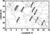 |
Figure 1 Geographical distribution of the European ionosonde network used in HF-INT. |
Geographic coordinates, sampling cadence, and ionosonde model of each station in the network.
It should be noted that the HF-INT provides information about the activity of LSTIDs detected on the locations of the different ionosonde sensors that make up the observation network, i.e., the HF-INT data over a single ionosonde location. Furthermore, considering that LSTIDs are large-scale phenomena, it also provides information about the activity of LSTIDs over the region, considered as a whole, encompassed by the ionosonde network, i.e., the HF-INT data over the region of the ionosonde network.
2.1 HF-INT data over a single ionosonde location
According to the LSTID detection criteria described in Altadill et al. (2020), HF-INT runs every 5 min, providing the following LSTID characteristics: wave period, spectral power, amplitude, spectral energy contribution (SEC), magnitude and direction (azimuth) of perturbation propagation velocity for every sensor. Additionally, HF-INT classifies LSTID activity according to the SEC of the detected disturbance. The SEC of a given LSTID quantifies the disturbance’s contribution to total time series variability (Altadill et al., 2020). Therefore, the larger the SEC of an LSTID, the larger the impact of the disturbance on the variability. The classification of LSTID activity has been calibrated using data from 2018, a year with moderate solar activity and reliable data availability for all ionospheric sensors. The different levels of activity were determined from the complementary cumulative distribution function of the SEC (Fig. 2) and are indicated by a “Traffic Light” integer number for each sensor (TrLi), ranging from 1 to 5. The quartiles/deciles shown in Figure 2 were chosen as they best describe the intensity of the detected TIDs. The ninth decile of the distribution defines Insignificant activity (SEC < 18% and TrLi = 1). The median defines Weak activity (18% ≤ SEC < 65% and TrLi = 2). The first quartile defines Moderate activity (65% ≤ SEC < 80% and TrLi = 3). The first quartile to the first decile defines Strong activity (80% ≤ SEC < 86% and TrLi = 4). The first decile defines Very Strong activity (SEC ≥ 86% and TrLi = 5). We must indicate that the distribution in Figure 2 refers to cases where certain LSTID activity was detected during 2018, representing 20% of the total scenarios. We refer to as a scenario all possible detection activities every 5 min in 2018 and for each ionosonde sensor. The remaining 80% of the 2018 scenarios, which are not considered in Figure 2, fall into the category of no activity or lack of sufficient data for analysis and are assigned an activity level TrLi = 0.
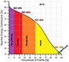 |
Figure 2 Complementary cumulative number of events for a given SEC of LSTID scenarios detected in 2018. |
2.2 HF-INT data for the region of the ionosonde network
HF-INT data from single ionosonde locations are used to provide a wider HF-INT activity index for the region encompassing the European network, referred to as HF-INTEU, in addition to the local levels of LSTID activity at individual ionosonde locations within the network (TrLi). HF-INTEU is obtained as the product of the average warning level indicators (TrLi) and the ratio of the number of stations in the network reporting weak activity or higher (Na) to the total number of stations providing measurements (N), which helps quantify the area of the European sensor network affected by LSTID:
 (1)
(1)
where TrLi represents the warning level indicator at each single ionosonde location. HF-INTEU is time-dependent, as each time the method runs, every 5 min, a new index value is generated.
We established different levels of LSTID activity for the European region, i.e. TID category HF-INTEU ≥ 1.75 (scenarios within the first decile of the occurrence distribution), the Uncertain category for 0.9 ≤ HF-INTEU ≤ 1.75 (scenarios between the first decile and the first quartile of the occurrence distribution), and the No TID category for HF-INTEU < 0.9 (scenarios outside the first quartile of the occurrence distribution). These categories are defined using the complementary cumulative number of events distributions, with HF-INTEU values at or below a threshold (Fig. 3). These thresholds result from the analysis carried out for the years 2014–2018 and, although not shown here, the quartiles/deciles were obtained as the optimum threshold values to detect LSTIDs with a minimum of false positives. The final drop in the curve shown in Figure 3 is due to the HF-INT restrictions on data availability. Note that estimating the vector velocity requires data from at least three stations; therefore, events with less data availability are rejected, causing the HF-INTEU to suddenly drop to 0.
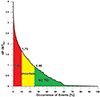 |
Figure 3 Complementary cumulative number of events depending on their HF-INTEU values. |
A detailed verification of LSTID existence based on the HF-INTEU index has been carried out. To this end, all LSTID activity maps whose HF-INTEU category corresponds to “Uncertain” or “TID” have been checked, verifying whether the propagation direction (azimuth) of the LSTID is consistent for all ionosonde locations reporting activity. To avoid spikes and ensure a true LSTID detection, the HF-INTEU must report continuous activity for at least the time corresponding to half of the dominant oscillation period of the TID, and, simultaneously, the propagation azimuths estimated over ionosonde locations must remain stable in the same quadrant for most of the stations and for that time interval.
As an example, Figure 4 illustrates two cases with high HF-INTEU values, but different azimuth patterns. On the left (Fig. 4a), the azimuth is coherent across all stations reporting activity. In contrast, on the right (Fig. 4b), the azimuth presents non-coherent behavior. Thus, the first event is considered to be classified as a real LSTID. On the contrary, it is evident that Figure 4b indicates some disturbance activity, but the non-coherent direction of propagation indicates that such disturbance does not correspond to a large-scale event. Thus, it could be caused by different reasons, such as multiple sources of TIDs, different MSTIDs in distinct regional areas, or situations where the assumptions of the method, such as plane wave propagation, are not valid. As a result, the origin of the perturbation and its propagation cannot be confirmed, and such a case type was not considered an LSTID event.
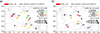 |
Figure 4 Two timestamps of HF-INT results for two different periods with high HF-INTEU values. In both cases, the maps show the same behavior during 3 h for the event on the left, and during 2.5 h for the event on the right. Arrows indicate propagation azimuth, with numbers representing velocity in m/s. |
Once the events with coherent azimuth have been selected, an average of the main TID characteristics, such as period, amplitude, SEC, velocity, and azimuth, is calculated for all stations for an instant of time, obtaining a value of these characteristics every 5 min. After that, an average over the whole duration of the event is taken to obtain a single value for each characteristic of the particular TID event. The averages of velocity and azimuth are computed taking into consideration their vector behavior. This way, the LSTID activity in near-real time has been analyzed in depth, resulting in a Catalogue of observed LSTID events that provides onset time, duration, dominant period, dominant amplitude, SEC, and propagation velocity vector for each event. It is important to note that the onset time of a reported LSTID in the catalog has an intrinsic delay that is due to the latency time required to observe the LSTID on a minimum number of sensors and that all of the above conditions are met. This HF-INT LSTID event Catalogue is available in Segarra et al. (2024). The LSTIDs events Catalogue includes 1848 events for the period 2014–2023, which means approximately one event every 2 days on average. As we will show later, the distribution of events is concentrated in specific time periods.
In this study, we will characterize LSTIDs over the period 2014–2023 to identify some climatological features. For that purpose, the Catalogue dataset, the single values for each event, is used to obtain the climatology of average characteristics of the LSTIDs for the region of the ionosonde network. However, HF-INT data over a single ionosonde location, which has been used to calculate the average characteristics for the duration of each TID event comprising the LSTIDs Catalogue, will be the basis for assessing detailed patterns of LSTID activity.
3 Results
This section presents the main features obtained from a statistical analysis of the results of HF-INT for the years 2014–2023. First, we provide statistics about the activity detected over the network and its primary characteristics. Second, we show the characteristics of LSTID propagation parameters, including their seasonal and local time dependencies.
3.1 Climatology of the average characteristics of the LSTIDs for the region of the ionosonde network
Figure 5 shows histograms of the occurrence of LSTID events reported in the Catalogue (HF-INT data for the region of the ionosonde network) as a function of the following characteristics: day of the year, onset time, SEC, wave period, velocity, and azimuth (Figs. 5a–5f, respectively). In Figure 5a, the histogram shows the seasonal activity of LSTIDs, which presents two maxima close to equinoxes and two minima in summer and winter. The observed summer activity minimum (Fig. 5a) may be somewhat biased due to the effect on the quality and availability of the MUF(3000)F2 data caused by the blanketing Es layers, which often make MUF measurements impossible in ionograms. This effect might be important in the daytime of summers when the Es occurrence is larger at middle latitudes (e.g., Davies, 1990; Haldoupis, 2012), and especially for low solar activity years, when the F2 layer density is low. The onset time histogram (Fig. 5b) reveals two maxima at sunrise and evening-midnight. The maximum sunrise is probably caused by the solar terminator effect. Figure 5c shows histograms of SEC, with the distribution peaking around 65–70%, which is an indication of the significant impact that LSTIDs cause in the variability of the ionosphere. The period distribution (Fig. 5d) indicates that the dominant period of the LSTIDs is centered around 120 min. The velocity distribution (Fig. 5e) is concentrated between 600 m/s and 700 m/s, in agreement with typical LSTIDs values reported in the literature (e.g. Tsugawa et al., 2004; Kishore & Kumar, 2023; Nykiel et al., 2024). The azimuth distribution (Fig. 5f) exhibits a primary peak around 180°, indicating a dominant southward propagation, potentially linked to an auroral origin, and a smaller peak around 270°, indicating westward propagation, suggesting a potential solar terminator origin.
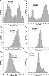 |
Figure 5 Histograms of occurrence of the LSTID Catalogue events for day of the year (a), local time of detection (b), SEC (c), period (d), velocity (e), and azimuth (f). |
3.2 Detailed patterns of LSTID activity
As noted earlier, HF-INT data over a single ionosonde location corresponding to each event in the LSTID Catalogue has been used to study in detail the activity patterns of the LSTIDs. The distribution of the occurrence of LSTID, year-by-year, as a function of local time and season is depicted in the first column of Figure 6. The data in Figure 6 have been binned by months (from 1 to 12, representing January to December) and local time (from 0 to 23). Event frequency is calculated as the percentage of scenarios showing LSTID activity. Note that, taking into account that HF-INT works every 5 min using data from 10 locations, the total number of possible scenarios in each data bin is approximately 3650, with an annual total of 1.05 million. To illustrate the relationship between LSTIDs and periods of high geomagnetic activity, we compared LSTIDs occurrence with geomagnetic activity occurrence exceeding certain thresholds. For this purpose, we utilized the Kp index (Matzka et al., 2021) and AE index (Nose et al., 2015) as indicators of geomagnetic activity. Kp reflects the global energy input into the magnetosphere from solar activity, while AE is associated with the energy deposited in the auroral region and is particularly sensitive to substorm activity. Figure 6 also shows the occurrence of Kp ≥ 3 for the same time interval (second column in Fig. 6) and the occurrence of AE index equal to or greater than 750 nT (third column in Fig. 6). Note that Figure 6 is arranged by rows, with each row corresponding to a specific year under study, with the bottom row showing the average over years 2014–2023. However, although the AE index is available in graphical form up to the present, numerical data for analysis is available only for 2014–2019. Consequently, results for the AE index are not shown for 2020–2023 or the overall average from 2014 to 2023. The highest LSTID occurrences are observed during equinoxes, particularly from dusk to dawn, and two minimums during solstices. Around the equinoxes, almost one LSTID is detected every 3 days. Higher occurrence rates are also observed for years with elevated geomagnetic activity (2014, 2015, 2022, and 2023). Note that the number of LSTID detections is lower in solstices, especially during daytime. The observations during summer can be somewhat biased because the occurrence of the Es layer, whose potential screening effects often make MUF(3000)F2 measurements impossible in ionograms, affects the detection of TIDs by HF-INT. However, during years of high geomagnetic activity, sufficient data is available for detection, which in turn makes the summer minimum less pronounced in those years.
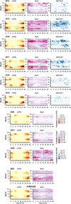 |
Figure 6 First column: Probability (%) of LSTID event frequency over all stations of the network for each year and the average for all years (bottom panel). Second column: Probability (%) of Kp equal to or greater than 3 for the same years and the average over all years (bottom panel). Third column: Probability (%) of AE equal to or greater than 750 nT for the years 2014 through 2019. |
We analyzed the LSTID activity compared to solar activity. We use the sunspot number from the Sunspot Index and Long-term Solar Observations (WDC-SILSO6) from the Royal Observatory of Belgium as a solar cycle indicator and the number of Sudden Commencements, from the International Service on Rapid Magnetic Variations (SRMV), hosted at Ebro Observatory7, as an indicator of geomagnetic activity. Figure 7 compares those activities for LSTID with dominant southward propagation (azimuth between 150° and 220°). We assume these LSTIDs to have an auroral origin and should be influenced by the solar cycle. The number of auroral-origin LSTIDs included in the catalog (black line) generally follows the trend of solar activity indicators, such as the sunspot number (red line) and the number of Sudden Storm Commencements and Sudden Impulses (SSC+SI, blue line). The lower LSTID occurrence around 2019–2020 aligns with the solar minimum, while the rise in solar activity from 2021 onward is accompanied by an increase in detected LSTIDs. The trend of the LSTID activity agrees much better with that of the number of SSCs and SIs. This is especially clear for the descending phase of solar cycle 25 (2014–2019). The latter results agree with the enhanced 27-day recurrent activity during the declining phase of even-numbered solar cycles (Ondoh & Nakamura, 1980) and with the fact that most of the largest geomagnetic storms occurred in the declining phase of the solar cycle (Araki, 2014).
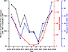 |
Figure 7 Temporal variation of auroral-origin LSTID occurrence (black line and left-hand y-axis) compared with solar activity indicators: sunspot number (red line and correspondingly the red y-axis on the right-hand side) and the number of Sudden Storm Commencements and Sudden Impulses (SSC+SI, blue line and correspondingly the blue y-axis on the right-hand side). |
HF-INT data over a single ionosonde location corresponding to each and every event in the LSTID Catalogue has also been used to study in detail the propagation patterns of the LSTIDs. In the Catalogue, there is an average of velocity and azimuth for the whole duration of the event, and sometimes, if the LSTID remains for many hours, the azimuth slightly changes during the event. The distribution of the LSTIDs as a function of the magnitude and the azimuth of propagation velocity is shown in Figure 8 in the form of a polar plot. This distribution has been binned into different cells of 100 m/s in the radial dimension (velocity magnitude) by 30° in the angular dimension (propagation azimuth). Note that an azimuth equal to zero indicates northward propagation, and the reference rotation direction is clockwise. The probability for each cell has been calculated as the percentage of events detected in each bin out of the total number of events that show LSTID activity. According to Figure 8, the dominant propagation velocity of LSTIDs has a magnitude of about 600 m/s and a dominant azimuth at around 180°, suggesting a dominant auroral origin.
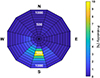 |
Figure 8 Polar plots of the distribution of the LSTIDs as function of the propagation velocity. |
The results of Figure 8 are somewhat different from those of Figure 5b. The secondary maximum of LSTIDs with westward propagation azimuth observed in Figure 5b is almost imperceptible in Figure 8. To try to explain this fact, a more in-depth analysis has been performed, discriminating the distribution of the occurrence of LSTIDs as a function of the magnitude and azimuth of the propagation velocity by four-time sectors (Fig. 9). Thus, Figure 9a shows the distribution of LSTIDs as a function of their propagation speed for the 21–03 UT sector, Figure 9b for the 03–09 UT sector, Figure 9c for the 09–15 sector, and Figure 9d for the 15–21 UT sector; that is, they are centered approximately at midnight, sunrise, noon, and sunset respectively. Similarly to Figure 8, the probability for each cell has been calculated as the percentage of events detected in each bin out of the total number of events that show LSTID activity for the respective time sector. Results of Figure 9 show that LSTIDs detected in the time sectors from 09 to 03 UT (Figs. 9a, 9c, and 9d) exhibit a dominant southward propagation with velocities around 600 m/s. However, LSTIDs detected in the sector from 03 to 09 UT (centered on the sunrise) show a dominant westward propagation with velocities around 400 m/s. This differential fact in the speed of propagation of LSTIDs supports different sources of origin, being consistent as a dominant origin in the auroral activity for the LSTIDs detected in the sectors between 09 and 03 UT, while the LSTIDs detected in the sector from 03 to 09 UT supports a dominant origin in the sunrise solar terminator.
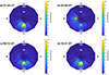 |
Figure 9 Polar plots of the distribution of the LSTIDs as function of the propagation velocity for four time sectors. |
Note also that the velocity magnitude of LSTIDs detected in the sunrise sector is lower than those detected in the remaining sectors and is closer to typical MSTID velocities. Furthermore, although not shown here, TID events detected in the sunrise sector have typically shorter durations than LSTIDs detected in the other sectors and affect fewer ionosonde locations simultaneously. These observational findings support the idea that TIDs detected in the sunrise sector have a dominant origin in the sunrise solar terminator and could be qualified as MSTIDs.
We have also studied in detail the distribution of LSTIDs as a function of propagation velocity at different seasons. Although not shown here, the distribution of LSTIDs as a function of propagation velocity shows a similar pattern under different seasonal conditions for the LSTIDs detected in sectors 09–03 UT, observing a clear dominant southward propagation with velocities around 600 m/s; a pattern like that reported in Figures 9a, 9c, and 9d, respectively. However, the TIDs detected in the sunrise sector show a different pattern in the distribution of the LSTIDs depending on the propagation velocity for different seasons. Figure 10 shows the distribution of LSTIDs detected in the sunrise sector as a function of the propagation velocity discriminated by four different seasons: winter (November–January, Fig. 10a), spring (February–April, Fig. 10b), summer (May–July, Fig 10c), and fall (August-October, Fig. 10d). Similarly to Figure 9, the probability for each cell of Figure 10 has been calculated as the percentage of events detected in each bin out of the total number of events that show LSTID activity for the respective season at the given time sector.
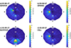 |
Figure 10 Polar plots of the distribution of the LSTIDs detected in the time sector 03–09 UT as function of propagation velocity for different seasons. |
Results show that LSTIDs detected in the sunrise sector during winter observe a dominant westward propagation, slightly tilted to the north (NWW), with velocities around 400 m/s (Fig. 10a). LSTIDs detected in the sunrise sector during spring (Fig. 10b) and fall (Fig. 10d) exhibit a dominant westward propagation with velocities around 400 m/s. However, LSTIDs detected in the sunrise sector during summer (Fig. 10c) observe a dominant southward propagation with velocities at about 600 m/s. The different patterns of propagation of LSTIDs for the sunrise sector during different seasons might indicate the different sources and driving mechanisms. We can therefore speculate that the dominant source of LSTIDs in the equinoxes for the sunrise sector is related to the solar terminator, which is coherent with a dominant westward propagation. The solar terminator also appears to be the dominant source of LSTID in winter for the sunrise sector. In this case, the dominant NWW propagation direction could be attributed to the combined effect of the westward propagation of the solar terminator and the meridional circulation of the thermosphere from the summer to the winter hemisphere. Observations indicate a potential influence of the solar terminator tilt angle on the propagation direction. The LSTID propagation pattern for the sunrise sector during summer is significantly different from the rest of the seasons. In this case, the dominant southward propagation direction is not an indication that the terminator is the source of these LSTIDs. On the contrary, the dominant southward propagation suggests an origin in auroral activity. Thus, we could speculate that the solar terminator does not cause such sharp gradients in summer as to generate LSTIDs so significantly compared to the rest of the seasons, and that is why auroral-driven LSTIDs dominate in the sunrise sector during summer.
4 Discussion
Numerous statistical analyses evidence that the intensity and occurrence rate of LSTIDs are highly correlated with the magnetic activity over different longitudinal regions (e.g., Tsugawa et al., 2004; Ding et al., 2008; Borries et al., 2009). However, many LSTIDs propagating near-equatorward from auroral latitudes were also detected under non-magnetic storm conditions (Tsugawa et al., 2004; Zhang et al., 2021). In this study, we focused on the patterns of LSTIDs detected by HF-INT, showing the significant agreement between major LSTID occurrence and elevated values of geomagnetic indices such as Kp and AE. Interestingly, we observed LSTIDs with similar characteristics at different onset times of the day and under different space weather conditions: two maxima in the seasonal distribution of the LSTIDs around the equinoxes (Fig. 5a), and two maxima in the distribution of the onset time of the LSTIDs at around sunrise and the evening-midnight (Fig. 5b). To validate this observation, we present a statistical comparison for the seasonal and onset distribution across different years. For that purpose, the Catalog dataset of the LSTIDs for the region of the ionosonde network has been used. Thus, we considered those events in the catalogue for a particular year with potential auroral origin (150° < azimuth < 220°) and the different distributions of observables that can be derived from the catalogue. To assess whether the distribution of the seasonal activity of LSTIDs (Fig. 5a) and the distribution of the onset time of LSTIDs (Fig. 5b) remain consistent across the years, two-sample Kolmogorov-Smirnov (KS) tests (Feller, 1948; Press et al., 1992) were performed for different pairs of yearly samples. By assuming a significance level of 0.05, the p-values from the KS tests determine whether the differences in the seasonal and onset time distributions of LSTIDs are statistically significant. To further support the hypothesis of stationarity in LSTID occurrence, Figures 11 and 12 present a statistical analysis of the KS test results for all pairs of yearly samples under study. The horizontal and vertical axes of the matrix of Figures 11 and 12 represent the years, ny and nx in each box indicate the number of LSTID events detected for year y and x, respectively, and the top number in each box corresponds to the p-value from the KS test. The boxes are color-coded according to the p-values: A blue-colored box indicates that the distribution of the seasonal (Fig. 11) or of the onset time (Fig. 12) occurrences show no significant differences between the two-yearly samples represented on the x and y axes, whereas a reds colored box means that the distributions show significant differences between the two-yearly samples. It should be noted that the matrix is symmetric by definition.
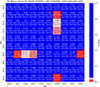 |
Figure 11 p-values of the KS tests for the yearly samples of the seasonal occurrence of LSTIDs. Numbers at the top correspond to the p-values of the KS test, and ny and nx correspond to the number of LSTID events for the years in the y and x axes, respectively. Boxes are colored from blue (non-significant discrepancies) to red (significant discrepancies) for a significance level of 0.05. |
The KS test indicates that no significant differences in the seasonal distribution of LSTID activity with potential origin in the auroral activity are observed along the years studied, apart from 2020 (Fig. 11). So, we can conclude that the seasonal distribution of the southward propagating LSTID is statistically significant. 2020 is the year with the lowest LSTID activity of the series, and its seasonal distribution of LSTID activity especially disagrees with that of the years 2015, 2016, 2017, and 2023. 2015 to 2017 are precisely the years with the highest magnetic activity as well as the highest LSTID activity, and 2023 reports significant geomagnetic and LSTID activity compared to 2020 (Fig. 6). The latter, and especially the very low number of detected LSTID events in 2020, can be a reason explaining the different seasonal distribution of LSTID activity.
The results of the KS test depicted in Figure 12 indicate that 2014 and 2015 show significant differences in the distribution of the onset time of LSTIDs with potential origin in the auroral activity compared to other years of the time series. Despite that, most of the years report statistically significant distribution of the onset time of LSTIDs with potential origin in the auroral activity. However, the distribution of the onset time of LSTIDs for 2014 disagrees with that of the years 2017 to 2022, and that of 2015 disagrees with that of 2018 to 2020 and 2021. Although not shown here, we evaluated the distribution of the onset of LSTIDs with potential auroral origin year by year and observed that all years report the onset of LSTIDs to dominantly occur from 16 to 23 UT. Only a few LSTID events with southward propagation start between 06 and 16 UT for all the years. The only difference between the years 2014 and 2015 in the distribution of the onset of the southward propagating LSTIDs is that these years report a significant number of LSTIDs starting between 00 and 06 UT, whereas the others did not. Thus, we can conclude that the onset distribution of the southward propagating LSTID activity is statistically significant.
In consistency with the neutral wind-based storm scenario, as long as auroral energy input is present, positive and negative effects in the ionosphere can be generated and drive TIDs (e.g. Prölss, 1993; Fuller-Rowell et al., 1994). Paznukhov et al. (2009) estimated the local time dependence of the ionospheric storm effects, showing distinctly different local time patterns for negative and positive ionospheric storms. Their results suggest that the composition disturbance zone responsible for the negative ionospheric storms tends to form around the sector of 0300–0500 LT and that the positive ionospheric storms prefer to begin around local noontime. Keeping in mind the latency time needed to detect a LSTID by the HF-INT (at least the time equivalent to one period of the detected LSTID), the results we have obtained for the onset distribution of LSTIDs propagating southward are not only statistically significant but consistent with also with neutral wind-based ionospheric storm scenario.
Thanks to the extensive HF-INT dataset, we have been able to describe the local time, seasonal, and solar activity dependence of LSTIDs occurrence. In agreement with the literature, we found typical LSTIDs periodicities of about 120 min, velocities around 600–700 m/s, and azimuths indicating southward propagation. The most remarkable observational finding is the near-daily occurrence of LSTIDs close to the equinoxes, detected by HF-INT under both disturbed and quiet geomagnetic conditions. This suggests high-latitude thermosphere experiences energy inputs, albeit weak, from the magnetosphere during quiet times, generating LSTID. The larger occurrence can be attributed to higher geomagnetic activity during equinoxes. Moreover, the propagation of LSTID is also influenced by the configuration of thermospheric and neutral winds during equinoxes, which facilitates the southern propagation of the effects caused by Joule heating in the auroral oval.
Another key topic of this study is the role of the solar terminator in the LSTID generation and propagation. The passage of the solar terminator can trigger a peak in LSTID activity during the morning hours (Song et al., 2013). In this study, we reported solar terminator-induced LSTIDs with predominant west-northwestward propagation and velocities of about 400 m/s in the 03–09 h time sector. Galushko et al. (1998) also observed propagation velocities near the terminator velocity at ionospheric heights (around 360 m/s) and westward propagation perpendicular to the solar terminator. They argued that the observations support theoretical predictions of TID generated by the solar terminator, according to the model described in Somsikov (1983). According to the classical TID classification Hunsucker (1982), a velocity of 400–300 m/s is on the boundary between MSTIDs and LSTIDs, but given their large extent over Europe, we considered them as LSTIDs. The variation in propagation azimuth with the seasons further confirms the solar terminator as a source of these LSTIDs.
Equally noteworthy is the absence of observable effects related to the sunset terminator. Several studies have reported stronger effects at the sunrise terminator than at the sunset terminator for different ionospheric parameters, including electron temperature (Raitt &Clark 1973), TIDs (Galushko et al., 1998; MacDougall & Jayachandran 2011; Song et al., 2013), and short-term electron density variability in the F region (Boška et al., 2003). Using TEC measurements from GPS data, Afraimovich (2008) found that “wave packets” were more pronounced at sunrise than at sunset. According to Somsikov (2011), the characteristic width of the sunrise solar terminator is much smaller than that of the sunset, due to the powerful processes of photoionization and atmospheric heating occurring at sunrise, making it a more efficient generator of AGWs. Besides these arguments, the LSTID climatology observed by the HF-INT indicates a dominant southward propagation in the afternoon and nighttime sectors. The latter does not exclude the possibility of observe eastward propagating events at the sunset sector, but these are much less significant (Fig. 9d).
5 Conclusions
This study has provided a detailed analysis of the characteristics and patterns of LSTIDs over Europe for the period 2014–2023 using HF-INT. The results made it possible to build a detailed Catalogue of LSTIDs for the European region. Based on this Catalogue, a consistent relationship between LSTID occurrence and geomagnetic activity has been demonstrated. However, under quiet geomagnetic conditions, a pronounced increase in activity during equinoxes has been reported, particularly at night and in the early morning. The study reveals that LSTIDs can occur under both disturbed and quiet geomagnetic conditions, suggesting the influence of the neutral wind conditions in the propagation of the Joule heating effect to southern latitudes during the equinox epoch.
Seasonal and temporal variations in LSTID propagation characteristics were observed, with significant southward propagation linked to auroral activity and westward propagation associated with the solar terminator. These findings highlight the complex dynamics governing LSTID behavior and emphasize the importance of continuous monitoring and analysis to better understand their impact on ionospheric conditions.
This research contributes valuable insights into the climatology of LSTIDs and their implications for communication systems and space weather forecasting. The results obtained in this study may be useful for modeling and predicting LSTID activity. Future work will focus on studying cases of unexpected propagation using specific event analyses. This will help identify and characterize the sources and conditions that lead to atypical LSTID behavior, potentially improving our predictive capabilities and understanding of the mechanisms driving these disturbances.
Acknowledgments
The paper uses ionospheric data from the Global Ionosphere Radio Observatory, which includes the USAF NEXION Digisonde network, the NEXION Program Manager is Annette Parsons. It also includes data from the ionospheric observatory in Roquetes, Spain, owned and operated by the Fundació Observatori de l’Ebre, as well as data from the Juliusruh Ionosonde, owned by the Leibniz Institute of Atmospheric Physics Kuehlungsborn, with Jens Mielich as the responsible Operations Manager. Additionally, it includes data from the ionospheric observatory in Dourbes, owned and operated by the Royal Meteorological Institute (RMI) of Belgium. We extend our gratitude to the national institutions and data providers that support them. We also thank GFZ Postdam for providing Kp index, Kyoto World Data Center for the AE index, the WDC-SILSO, Royal Observatory of Belgium, for the sunspot number, and the SRMV, Observatori de l'Ebre, for the Sudden Commencement data. The editor thanks Wenbin Wang and Rezy Pradipta for their assistance in evaluating this paper.
Funding
This research has been funded by EU Projects PITHIA-NRF (GA 101007599) and T-FORS (GA 101081835), in which V.N-P, D.A., A.S., and V.dP are participating.
Data availability statement
Data from ionosondes are available at: https://giro.uml.edu/didbase/scaled.php.
Geomagnetic indices Kp and AE are available respectively at: https://www.gfz.de/en/section/geomagnetism/data-products-services/geomagnetic-kp-index and https://wdc.kugi.kyoto-u.ac.jp/aedir/index.html.
Sunspot number is available at: https://www.sidc.be/SILSO/datafiles.
Event lists of SSC are available at: https://www.obsebre.es/en/variations/rapid.
LSTID catalogue is available at: https://doi.org/10.34810/data1383.
References
- Afraimovich EL. 2008. First GPS-TEC evidence for the wave structure excited by the solar terminator. Earth Planets Space 60: 895–900. https://doi.org/10.1186/BF03352843. [CrossRef] [Google Scholar]
- Altadill D, Segarra A, Blanch E, Juan JM, Paznukhov V, Buresova D, Galkin I, Reinisch BW, A Belehaki. 2020. A method for real-time identification and tracking of traveling ionospheric disturbances using ionosonde data: First results. J Space Weather Space Clim 10: 2. https://doi.org/10.1051/swsc/2019042. [CrossRef] [EDP Sciences] [Google Scholar]
- Araki T. 2014. Historically largest geomagnetic sudden commencement (SC) since 1868. Earth Planets Space 66: 164. https://doi.org/10.1186/s40623-014-0164-0. [CrossRef] [Google Scholar]
- Belehaki A, Tsagouri I, Altadill D, Blanch D, Borries C, et al. 2020. An overview of methodologies for real-time detection, characterisation and tracking of traveling ionospheric disturbances developed in the TechTIDE project. J Space Weather Space Clim 10: 42. https://doi.org/10.1051/swsc/2020043. [CrossRef] [EDP Sciences] [Google Scholar]
- Borries C, Jakowski N, Wilken V. 2009. Storm induced large scale TIDs observed in GPS derived TEC. Ann Geophys 27(4): 1605–1612. https://doi.org/10.5194/angeo-27-1605-2009. [CrossRef] [Google Scholar]
- Boška J, Šauli P, Altadill D, German Solé D, Alberca LF. 2003. Diurnal variation of gravity wave activity at midlatitudes in the ionospheric F region. Stud Geophys Geod 47: 579–586. https://doi.org/10.1023/A:1024763618505. [Google Scholar]
- Chilcote M, LaBelle J, Lind FD, Coster AJ, Miller ES, Galkin IA, Weatherwax AT. 2015. Detection of traveling ionospheric disturbances by medium-frequency Doppler sounding using AM radio transmissions. Radio Sci 50: 249–263. https://doi.org/10.1002/2014RS005617. [Google Scholar]
- Davies K. 1990. Sporadic E. In: Ionospheric radio, Peter Peregrinus Ltd., London, UK, pp.143–145. ISBN 086341186X. [Google Scholar]
- Ding F, Wan W, Liu L, Afraimovich E, Voeykov S, Perevalova N. 2008. A statistical study of Large‐scale Traveling Ionospheric Disturbances observed by GPS TEC during major magnetic storms over the years 2003–2005. J Geophys Res 113(A3): A00A01. https://doi.org/10.1029/2008JA013037. [Google Scholar]
- Essien P, Figueiredo CAOB, Takahashi H, Wrasse CM, Barros D, et al. 2021. Long-term study on medium-scale traveling ionospheric disturbances observed over the South American equatorial region. Atmosphere 12: 1409. https://doi.org/10.3390/atmos12111409. [CrossRef] [Google Scholar]
- Evans JV, Holt JM, Wand RH. 1983. A differential-Doppler study of traveling ionospheric disturbances from Millstone Hill. Radio Sci 18: 435–451. https://doi.org/10.1029/RS018i003p00435. [Google Scholar]
- Feller W. 1948. On the Kolmogorov-Smirnov limit theorems for empirical distributions. Ann Math Statist 19(2): 177–189. [CrossRef] [Google Scholar]
- Ferreira AA, Borries C, Xiong C, Borges RA, Mielich J, et al. 2020. Identification of potential precursors for the occurrence of Large-Scale Traveling Ionospheric Disturbances in a case study during September 2017. J Space Weather Space Clim 10: 32. https://doi.org/10.1051/swsc/2020029. [Google Scholar]
- Fuller-Rowell TJ, Codrescu MV, Moffett RJ, Quegan S. 1994. Response of the thermosphere and ionosphere to geomagnetic storms. J Geophys Res 99: 3893–3914. https://doi.org/10.1029/93JA02015. [CrossRef] [Google Scholar]
- Fukao S, Yamamoto Y, Oliver WL, Takami T, Yamanaka MD, Yamamoto M, Nakamura T, Tsuda T. 1991. Middle and upper atmosphere radar observations of ionospheric horizontal gradients produced by gravity waves. J Geophys Res 98: 9443–9451. https://doi.org/10.1029/92JA02846. [Google Scholar]
- Galushko VG, Paznukhov VV, Yampolski YM, Foster JC. 1998. Incoherent scatter radar observations of AGW/TID events generated by the moving solar terminator. Ann Geophys 16: 821–827. https://doi.org/10.1007/s00585-998-0821-3. [CrossRef] [Google Scholar]
- Haldoupis Ch. 2012. Midlatitude Sporadic E. A typical paradigm of atmosphere-ionosphere coupling. Space Sci Rev 168: 441–461. https://doi.org/10.1007/s11214-011-9786-8. [Google Scholar]
- Haralambous H, Guerra M, Chum J, Verhulst TGW, Barta V, et al. 2023. Multi-instrument observations of various ionospheric disturbances caused by the 6 February 2023 Turkey earthquake. J Geophys Res Space Phys 128: e2023JA031691. https://doi.org/10.1029/2023JA031691. [CrossRef] [Google Scholar]
- Hines CO. 1960. Internal atmospheric gravity waves at ionospheric heights. Can J Phys 38(11): 1441–1481. https://doi.org/10.1139/p60-150. [CrossRef] [Google Scholar]
- Hocke K, Schlegel K. 1996. A review of atmospheric gravity waves and travelling ionospheric disturbances: 1982–1995. Ann Geophys 14: 917–940. https://doi.org/10.1007/s00585-996-0917-6. [Google Scholar]
- Hunsucker RD. 1982. Atmospheric gravity waves generated in the high-latitude ionosphere: a review. Rev Geophys Space Phys 20: 293–315. https://doi.org/10.1029/RG020i002p00293. [Google Scholar]
- Jacobson AR, Carlos RC, Massey RS, Wu G. 1995. Observations of traveling ionospheric disturbances with a satellite-beacon radio interferometer: seasonal and local time behavior. J Geophys Res 100: 1653–1665. https://doi.org/10.1029/94JA02663. [CrossRef] [Google Scholar]
- Kirchengast G, Hocke K, Schlegel K. 1996. The gravity wave-TID relationship: insight via theoretical model-EISCAT data comparison. J Atmos Terr Phys 58: 233–243. https://doi.org/10.1016/0021-9169(95)00032-1. [Google Scholar]
- Kishore A, Kumar S. 2023. Large scale traveling ionospheric disturbances during geomagnetic storms of 17 March and 23 June 2015 in the Australian region. J Geophys Res Space Phys 128: e2023JA031740. https://doi.org/10.1029/2023JA031740. [Google Scholar]
- MacDougall JW, Jayachandran PT. 2011. Solar terminator and auroral sources for traveling ionospheric disturbances in the midlatitude F region. J Atmos Terr Phys 73: 2437–2443. https://doi.org/10.1016/j.jastp.2011.10.009. [Google Scholar]
- Matzka J, Stolle C, Yamazaki Y, Bronkalla O, Morschhauser A. 2021. The geomagnetic Kp index and derived indices of geomagnetic activity. Space Weather 19: e2020SW002641. https://doi.org/10.1029/2020SW002641. [CrossRef] [Google Scholar]
- Morgan MG, Calderon CHJ, Ballard KA. 1978. Techniques for the study of TID’s with multi-station rapid-run ionosondes. Radio Sci, 13: 729–741. https://doi.org/10.1029/RS013i004p00729. [CrossRef] [Google Scholar]
- Nose M, Iyemori T, Sugiura M, Kamei T. 2015. Geomagnetic AE index. World Data Center for Geomagnetism, Kyoto. https://doi.org/10.17593/15031-54800. [Google Scholar]
- Nykiel G, Ferreira A, Gunzkofer F, Iochem P, Tasnim S, Sato H. 2024. Large‐Scale Traveling Ionospheric Disturbances over the European sector during the geomagnetic storm on March 23–24, 2023: Energy deposition in the source regions and the propagation characteristics. J Geophys Res Space Phys 129: e2023JA032145. https://doi.org/10.1029/2023JA032145. [CrossRef] [Google Scholar]
- Ondoh T, Nakamura Y. 1980. Solar cycle effect of 27-day recurrent geomagnetic storms. In: Solar-Terrestrial Predictions Proceedings, vol. IV, Donnely RF (Ed.), Space Environment Laboratory, Boulder, CO, pp. A-46–A-52. [Google Scholar]
- Paznukhov V, Altadill D, Reinisch BW. 2009. Experimental evidence for the role of the neutral wind in the development of ionospheric storms in midlatitudes. J Geophys Res 114: A12319. https://doi.org/10.1029/2009JA014479. [Google Scholar]
- Paznukhov V, Altadill D, Juan JM, Blanch E. 2020. Ionospheric tilt measurements: application to traveling ionospheric disturbances climatology study. Radio Sci 55: e2019RS007012. https://doi.org/10.1029/2019RS007012. [Google Scholar]
- Press WH, Teukolsky SA, Flannery BP. 1992. Numerical recipes in Fortran 77: the art of scientific computing, 2nd edn. Cambridge University Press, New York, USA. [Google Scholar]
- Prölss GW. 1993. Common origin of positive ionospheric storms at middle latitudes and the geomagnetic activity effect at low latitudes. J Geophys Res 98: 5981–5991. https://doi.org/10.1029/92JA02777. [CrossRef] [Google Scholar]
- Prölss GW, Ocko M. 2000. Propagation of upper atmospheric storm effects towards lower latitudes. Adv Space Res 26(1): 131–135. https://doi.org/10.1016/S0273-1177(99)01039-X. [CrossRef] [Google Scholar]
- Raitt WJ, Clark DH. 1973. Wave-like disturbances in the ionosphere. Nature 243: 508–509. https://doi.org/10.1038/243508a0. [Google Scholar]
- Reinisch BW, Galkin I, Belehaki A, Paznukhov V, Huang X, et al. 2018. Pilot ionosonde network for identification of traveling ionospheric disturbances. Radio Sci 53: 365–378. https://doi.org/10.1002/2017RS006263. [CrossRef] [Google Scholar]
- Reinisch BW, Galkin IA, Khmyrov GM, Kozlov AV, Bibl K, et al. 2009. New Digisonde for research and monitoring applications. Radio Sci 44: RS0A24. https://doi.org/10.1029/2008RS004115. [CrossRef] [Google Scholar]
- Reinisch BW, Galkin I. 2011. Global ionospheric radio observatory (GIRO). Earth Planets Space 63: 377–381. https://doi.org/10.5047/eps.2011.03.001. [CrossRef] [Google Scholar]
- Segarra A, Altadill D, de Paula V, Navas-Portella V. 2024. Catalogue LSTID. CORA.Repositori de Dades de Recerca, V1. https://doi.org/10.34810/data1383. [Google Scholar]
- Somsikov VM. 1983. Solar terminator and dynamics of the atmosphere. Nauka, Alma-Ata (former URSS). [Google Scholar]
- Somsikov VM. 2011. Solar terminator and dynamic phenomena in the atmosphere: A review. Geomagn Aeron 51(6): 707–719. https://doi.org/10.1134/s0016793211060168. [Google Scholar]
- Song Q, Ding F, Wan W, Ning B, Liu L, Zhao B, Li Q, Zhang R. 2013. Statistical study of large-scale traveling ionospheric disturbances generated by the solar terminator over China. J Geophys Res Space Phys 118(7): 4583–4593. https://doi.org/10.1002/jgra.50423. [CrossRef] [Google Scholar]
- Tsagouri I, Belehaki A, Koutroumbas K, Tziotziou K, Herekakis T. 2023. Identification of large-scale travelling ionospheric disturbances (LSTIDs) based on digisonde observations., Atmosphere 14: 331. https://doi.org/10.3390/atmos14020331. [CrossRef] [Google Scholar]
- Tsugawa T, Saito A, Otsuka Y. 2004. A statistical study of large-scale traveling ionospheric disturbances using the GPS network in Japan. J Geophys Res 109: A06302. https://doi.org/10.1029/2003JA010302. [CrossRef] [Google Scholar]
- Tsunoda RT, Cosgrove RT. 2001. Coupled electrodynamics in the nighttime midlatitude ionosphere., Geophys Res Lett 28: 4171–4174. https://doi.org/10.1029/2001GL013245. [Google Scholar]
- Verhulst TGW, Altadill D, Barta V, Belehaki A, Burešová D, et al. 2022. Multi-instrument detection in Europe of ionospheric disturbances caused by the 15 January 2022 eruption of the Hunga volcano. J Space Weather Space Clim 12: 35. https://doi.org/10.1051/swsc/2022032. [CrossRef] [EDP Sciences] [Google Scholar]
- Waldock JA, Jones TB. 1986. HF Doppler observations of medium-scale traveling ionospheric disturbances observed at mid-latitudes. J Atmos Terr Phys 48: 245–260. https://doi.org/10.1016/0021-9169(86)90099-1. [Google Scholar]
- Zhang R, Chen G, Li Y, Zhang S, Gong W, He Z, Zhang M. 2021. Long-term observation of the quasi-3-hour large-scale traveling ionospheric disturbances by the oblique-incidence ionosonde network in North China. Sensors 22(1): 233. https://doi.org/10.3390/s22010233. [Google Scholar]
Cite this article as: Segarra A, Altadill D, de Paula V & Navas-Portella V 2025. Climatology of large-scale Traveling Ionospheric Disturbances above Europe during the 2014–2023 period. J. Space Weather Space Clim. 15, 28. https://doi.org/10.1051/swsc/2025024.
All Tables
Geographic coordinates, sampling cadence, and ionosonde model of each station in the network.
All Figures
|
Figure 1 Geographical distribution of the European ionosonde network used in HF-INT. |
| In the text | |
|
Figure 2 Complementary cumulative number of events for a given SEC of LSTID scenarios detected in 2018. |
| In the text | |
|
Figure 3 Complementary cumulative number of events depending on their HF-INTEU values. |
| In the text | |
|
Figure 4 Two timestamps of HF-INT results for two different periods with high HF-INTEU values. In both cases, the maps show the same behavior during 3 h for the event on the left, and during 2.5 h for the event on the right. Arrows indicate propagation azimuth, with numbers representing velocity in m/s. |
| In the text | |
|
Figure 5 Histograms of occurrence of the LSTID Catalogue events for day of the year (a), local time of detection (b), SEC (c), period (d), velocity (e), and azimuth (f). |
| In the text | |
|
Figure 6 First column: Probability (%) of LSTID event frequency over all stations of the network for each year and the average for all years (bottom panel). Second column: Probability (%) of Kp equal to or greater than 3 for the same years and the average over all years (bottom panel). Third column: Probability (%) of AE equal to or greater than 750 nT for the years 2014 through 2019. |
| In the text | |
|
Figure 7 Temporal variation of auroral-origin LSTID occurrence (black line and left-hand y-axis) compared with solar activity indicators: sunspot number (red line and correspondingly the red y-axis on the right-hand side) and the number of Sudden Storm Commencements and Sudden Impulses (SSC+SI, blue line and correspondingly the blue y-axis on the right-hand side). |
| In the text | |
|
Figure 8 Polar plots of the distribution of the LSTIDs as function of the propagation velocity. |
| In the text | |
|
Figure 9 Polar plots of the distribution of the LSTIDs as function of the propagation velocity for four time sectors. |
| In the text | |
|
Figure 10 Polar plots of the distribution of the LSTIDs detected in the time sector 03–09 UT as function of propagation velocity for different seasons. |
| In the text | |
|
Figure 11 p-values of the KS tests for the yearly samples of the seasonal occurrence of LSTIDs. Numbers at the top correspond to the p-values of the KS test, and ny and nx correspond to the number of LSTID events for the years in the y and x axes, respectively. Boxes are colored from blue (non-significant discrepancies) to red (significant discrepancies) for a significance level of 0.05. |
| In the text | |
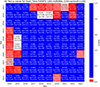 |
Figure 12 As in Figure 11, but for the onset occurrence of LSTIDs. |
| In the text | |
Current usage metrics show cumulative count of Article Views (full-text article views including HTML views, PDF and ePub downloads, according to the available data) and Abstracts Views on Vision4Press platform.
Data correspond to usage on the plateform after 2015. The current usage metrics is available 48-96 hours after online publication and is updated daily on week days.
Initial download of the metrics may take a while.