| Issue |
J. Space Weather Space Clim.
Volume 15, 2025
Topical Issue - Observing, modelling and forecasting TIDs and mitigating their impact on technology
|
|
|---|---|---|
| Article Number | 20 | |
| Number of page(s) | 13 | |
| DOI | https://doi.org/10.1051/swsc/2025014 | |
| Published online | 20 May 2025 | |
Technical Article
Assessment of models for the prediction of the Travelling Ionospheric Disturbance activity index in mid-latitude Europe
1
Institute for Solar-Terrestrial Physics, German Aerospace Center, 17235 Neustrelitz, Germany
2
Department of Electrical Engineering, University of Brasília, 70910-900 Brasília, Brazil
* Corresponding author: This email address is being protected from spambots. You need JavaScript enabled to view it.
Received:
11
April
2024
Accepted:
10
April
2025
Abstract
Given the impact the ionosphere electron density has on radio wave propagation, understanding, characterizing and predicting its behaviour and associated perturbations is of high importance. One type of perturbation commonly observed during geomagnetic storm events is the Large Scale Travelling Ionospheric Disturbance (LSTID). LSTIDs correspond to the ionospheric signature of large-scale atmospheric gravity waves that propagate in the thermosphere. Such waves, which are typically generated due to the input of energy from the solar wind into the Magnetosphere-Ionosphere-Thermosphere (MIT) system, are an essential component contributing to the development of ionospheric storms. Recently, the ATID index, which has been introduced for statistical analyses of TIDs, has been shown to correlate well with solar wind energy input in Europe in mid-latitude regions. The feasibility of predicting LSTIDs in this region has been demonstrated using a linear regression model. Here, an assessment of more advanced modelling approaches is presented to demonstrate their applicability and improvement of the predictions. This work applies methodologies based on artificial neural networks and multi-model ensembles. The persistence model is taken as a baseline for the performance assessment of the different methodologies. A given challenge for the generation of LSTID prediction models is the limited number of observations available. Still, the results show that all proposed methodologies outperform the baseline model when predicting the level of LSTID activity during geomagnetic storms over mid-latitude Europe for predictions beyond 1 h. The linear regression model shows in most cases the best performance among the investigated methodologies, evidencing that more complex techniques could not educe their capabilities in the application of LSTID prediction. For prediction times of 30 min, however, the ensemble of the linear regression and the persistence models presented the best performance overall. The presented assessment of LSTID prediction models/approaches contributes to the development of strategies for predicting LSTID activities over the European region and, it enhances the understanding of the strengths and limitations of different modelling methodologies for this use case.
Key words: LSTIDs activity / Forecasting / Solar Wind
© A.A. Ferreira et al., Published by EDP Sciences 2025
 This is an Open Access article distributed under the terms of the Creative Commons Attribution License (https://creativecommons.org/licenses/by/4.0), which permits unrestricted use, distribution, and reproduction in any medium, provided the original work is properly cited.
1 Introduction
Geomagnetic storms are closely related to the occurrence of disturbances in the thermosphere and ionosphere. The list of disturbances associated with geomagnetic storms includes for example, changes in the neutral and electron densities (Prölss, 1980; Mendillo, 2006; Codrescu et al., 2022), enhancement of ionospheric conductivities and currents (Buonsanto, 1999), and variations in the neutral winds (Fuller-Rowell & Codrescu, 1996; Jonah et al., 2020). During such events, a considerable amount of energy and momentum can be deposited in the auroral zone via enhanced electric fields, precipitation of particles, and Joule heating (Aa et al., 2019). The deposition of energy and momentum contributes to the triggering of wave-like perturbations in the ionospheric electron density that exhibit an apparent motion with horizontal velocities ranging from 400 up to 1000 m/s, periods varying from 30 min to 3 h and wavelengths greater than 1000 km. These perturbations are called Large Scale Travelling Ionospheric Disturbances (LSTIDs) and are the manifestation in the ionosphere of Atmospheric Gravity Waves (AGWs) generated due to auroral and geomagnetic activity (Hines, 1960; Hunsucker, 1982; Cherniak & Zakharenkova, 2018). For decades, TIDs and their theoretical understanding have been the subject of several investigations (Munro, 1948; Hines, 1960; Francis, 1975; Hocke & Schlegel, 1996) and different studies have been conducted in order to model, detect, and statistically characterize their occurrence using different instruments. Such investigations have included, for example, the use of ionosondes (Morgan et al., 1978; Maruyama et al., 2004; Reinisch et al., 2018), All-Sky imagers (Kubota et al., 2000; Otsuka et al., 2004) and Global Navigation Satellite Systems (GNSS) data (Saito et al., 1998; Tsugawa & Saito, 2004; Hernández-Pajares et al., 2006; Otsuka et al., 2013; Zakharenkova et al., 2016). In addition, significant efforts towards the modelling/prediction of TIDs using semi-empirical modelling approaches and general circulation models have been made (e.g., Mayr et al., 1990; Millward et al., 1993; Ridley et al., 2006; Fedorenko et al., 2013; Yokoyama, 2014; Sheng et al., 2020; Vadas et al., 2023; Bukowski et al., 2024). Despite the considerable progress in modelling/understanding TIDs, predicting them is still a challenging task due to the complexity of the coupling mechanisms in the thermosphere-ionosphere system. Recently, a new methodology for predicting TID activity over mid-latitude Europe during geomagnetic storms has been presented by Borries et al. (2023). This methodology is based on the use of a linear regression approach in order to predict the TID activity index (ATID). The index is derived from GNSS Total Electron Content (TEC) measurements and is also well-suited for statistical analysis and investigation of the source mechanisms of LSTIDs. The model uses solar wind data derived from Lagrangian point L1 as input, more specifically the Kan–Lee merging electric field. Results presented by Borries et al. (2023) have shown that the proposed approach outperforms the persistence model (PM) for predictions beyond 30 min for strong levels of TID activity (i.e. ATID ≥ 0.5 TECU).
The methodology proposed by Borries et al. (2023) is based on a linear regression approach and it has been proven to have a good performance in predicting LSTIDs activities at mid-latitudes. Different prediction methodologies have been developed throughout the years and applied in Space Weather research. Such methodologies may include, for example, neural networks (NNS, Haykin, 2009; Camporeale, 2019) and multi-model ensembles (Murray, 2018). In this context, we investigate to what extent state-of-the-art methodologies can improve the prediction of LSTID activity at mid-latitudes. For this purpose, we develop additional models for predicting the level of LSTID activity using NNs and multi-model ensemble approaches. The performance of the methodologies is evaluated in a set of different geomagnetic storms (see Appendix) and the geomagnetic storm observed on November 20, 2003 is used to illustrate how the methodology works.
This work is structured as follows: Section 2 presents the data used in this investigation and the methodologies proposed for predicting the LSTID activity. The results are presented in Section 3. The discussion of the results and the conclusions are presented in Sections 4 and 5, respectively.
2 Data and methodology
2.1 TID activity index (A TID )
As previously mentioned, TIDs can be detected from GNSS data. The slant TEC (sTEC) is obtained by combining carrier phase/code measurements at two frequencies f1 and f2, according to equations (1) and (2):![Mathematical equation: $$ \mathrm{sTEC}=\frac{{f}_1^2{f}_2^2}{40.3({f}_1^2-{f}_2^2)}\left[({\mathrm{\Phi }}_1-{\mathrm{\Phi }}_2)+{B}_{\mathrm{amb}}+{\epsilon }_{{\mathrm{\Phi }}_1-{\mathrm{\Phi }}_2}\right], $$](/articles/swsc/full_html/2025/01/swsc240017/swsc240017-eq1.gif) (1)
(1)
![Mathematical equation: $$ \mathrm{sTEC}=\frac{{f}_1^2{f}_2^2}{40.3({f}_1^2-{f}_2^2)}\left[\left({\mathrm{\Psi }}_2-{\mathrm{\Psi }}_1\right)+{\epsilon }_{{\mathrm{\Psi }}_2-{\mathrm{\Psi }}_1}\right], $$](/articles/swsc/full_html/2025/01/swsc240017/swsc240017-eq2.gif) (2)where Φ and Ψ correspond to carrier and code pseudoranges, respectively. Noises (e.g. thermal noise) are represented by
(2)where Φ and Ψ correspond to carrier and code pseudoranges, respectively. Noises (e.g. thermal noise) are represented by  and
and  . Bamb is the carrier-phase ambiguity. Additional terms, such as inter-frequency biases and multipath are not included for the sake of simplicity (Hoque & Jakowski, 2012).
For the TID detection, the slant TEC at an elevation angle ε is then converted to an equivalent vertical TEC (vTEC) in a thin-shell model of the ionosphere according to equation (3): (3)where Re is the Earth’s radius, h
i
is the height of the thin-shell model, assumed here to be 350 km. After removing the regular trend of the background vTEC of the ionosphere, one can obtain a perturbation TEC for each satellite-receiver link, which allows the identification of the TIDs. The removal of the regular trend of the vTEC can be done in different ways (e.g. polynomial fitting, moving average or other trend estimation approaches), with no significant difference between the methodologies (Borries et al., 2023).
(3)where Re is the Earth’s radius, h
i
is the height of the thin-shell model, assumed here to be 350 km. After removing the regular trend of the background vTEC of the ionosphere, one can obtain a perturbation TEC for each satellite-receiver link, which allows the identification of the TIDs. The removal of the regular trend of the vTEC can be done in different ways (e.g. polynomial fitting, moving average or other trend estimation approaches), with no significant difference between the methodologies (Borries et al., 2023).
Recently, a new TID index was proposed by Borries et al. (2023), which is obtained as an extension of the already established ways of detecting TIDs from GNSS measurements. The index can be used to monitor the TIDs activity and also to perform statistical analysis and prediction of such disturbances. In this case, the TEC variability obtained by a bandpass filtering (TECbp) in the range of 30–60 min is extracted by calculating the difference of moving averages with 60 and 30 min window size, as presented in equation (4)
 (4)where vTEC corresponds to the vertical TEC; T30 = 30 min/Δt and T60 = 60 min/Δt, with Δt corresponding to the sampling time. For each time step t, the TID activity index is obtained by taking the difference between the maximum TECbp and the minimum TECbp in a 60-minute window size centred on t and multiplying by 0.5, as presented in equation (5)
 (5)where t − (30 min/Δt) ≤ x ≤ t + (30 min/Δt) and F corresponds to a Gaussian function applied to reduce the impact of the values that are away from the centre of the 60-minute window.
The index can be used for individual GNSS stations, but can also be employed on the mapping of TIDs activity. It also allows the investigation of LSTIDs and MSTIDs. It is important to highlight that although a 30–60 minute bandpass filter is used to obtain the ATID index, other disturbances may also be reflected in the ATID, especially at high and low latitudes. The source of such disturbances cannot be distinguished from the index itself. However, at mid-latitudes, the impact of other disturbances on the ATID index is expected to be smaller than at high and low latitudes.
Correlation studies with several solar and geomagnetic indices, such as the Kan–Lee merging electric field (EKL) and Auroral Electrojet (AE) index, have shown that the magnitude of the LSTIDs at mid-latitudes is well correlated with them. Based on this information, in this work we propose different methodologies for predicting the TIDs activity using solar wind data from Lagrangian Point L1 as input. The description of each methodology is given in the following sections.
2.2 November 20, 2003 geomagnetic storm
In this investigation, we analyze the prediction of the TID activity index over a set of more than 50 geomagnetic storms (see Appendix). To illustrate the methodology, the geomagnetic storm that occurred on November 20, 2023 is used. Figure 1 presents the evolution of SYM-H, Bz, solar wind speed and AE index during the storm. This was a strong geomagnetic storm event, which was related to the occurrence of an Interplanetary Coronal Mass Ejection (ICME) (Zhang et al., 2007), which reached the Earth on the morning of November 20, 2003 and led to a SYM-H index of approximately −490 nT at around 18 UT. Figure 1b shows the Bz component of the interplanetary magnetic field, which increased to about 33 nT and turned southward for more than 12 h, reaching a minimum value of about −52 nT. A significant increase in the solar wind speed is observed at about 11:21 UT, reaching 766.3 km/s. A significant increase in the auroral electrojet index is also observed, reaching over 2000 nT during this period, which indicates a high level of auroral activity. This geomagnetic storm and the ionospheric and thermospheric responses associated with this event have been reported in several investigations (Meier et al., 2005; Crowley et al., 2006; Becker-Guedes et al., 2007; Borries et al., 2017).
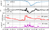 |
Figure 1 (a) SYM-H index, (b) Bz component of the interplanetary magnetic field, (c) solar wind speed and (d) AE index for 19–21 November, 2003. |
2.3 Persistence Model (PM)
The PM, although simple, is considered a useful prediction approach which assumes that the future value of a predicted variable is equal to the most recent observation (Reikard, 2018; Paulescu et al., 2021). In this case, the prediction of the TID activity ATID in a horizon prediction n, in minutes, is assumed to be equal to the most recent observation, i.e.  . This type of approach has been used for the prediction of different space weather parameters, such as solar radio flux, solar flare activity and the geomagnetic K-index (Devos et al., 2014). In this work, the PM is used as a baseline to evaluate the prediction performance of the proposed methodologies.
2.4 Linear Regression Models (LR)
The main goal of this analysis is to use the ATID to forecast TID activity in mid-latitudes, based on solar wind-derived parameters. It is therefore necessary to know which geophysical parameters or indices reflect the driving mechanisms for the generation of such disturbances. This analysis has been performed by Borries et al. (2023) by computing the cross-correlation of the ATID with different potential candidate parameters. The study separates two different types of geophysical parameters: geomagnetic indices and solar-wind magnetosphere coupling functions. In both cases, different parameters show a good correlation with the ATID index.
Although the investigation presented by Borries et al. (2023) analyses the correlation with 15 geophysical parameters and the TID activity index, in this work only the AE index and the Kan–Lee merging electric field are going to be used in the predictions, due to their high correlation shown in the previous study. It is important to highlight that other indices presented comparable correlations, such as the intermediate function (EWAV) and the modified version of the Akasofu index (ε3), but for simplicity, only the AE index and EKL are used here. In the LR models, the prediction of the TID activity is performed using a linear regression approach, with one of the aforementioned indices as input (AE index or EKL). A description of each one of these cases is given below.
2.4.1 LREKL
Borries et al. (2023) proposed LREKL and presented good results in predicting the TIDs activity using data from Lagrangian point L1. The methodology is based on the Kan–Lee merging electric field (EKL), which has been chosen due to its good performance in the study conducted in Newell et al. (2007), which investigated the geoeffectiveness of several parameters. In addition, the correlation studies conducted by Borries et al. (2023) have shown a correlation of 0.79 between the maximum ATID and the maximum EKL registered in the 18 h prior to the occurrence of the maximum ATID for different geomagnetic storms. Equation (6) describes the EKL coupling function (6)where v is the solar wind speed,
  is the transverse component of the Interplanetary Magnetic Field (IMF), with B
y
and B
z
corresponding to y and z components of the IMF and θ
c
= arctan(B
y
/B
z
) is the IMF clock angle.
is the transverse component of the Interplanetary Magnetic Field (IMF), with B
y
and B
z
corresponding to y and z components of the IMF and θ
c
= arctan(B
y
/B
z
) is the IMF clock angle.
The investigation presented by Borries et al. (2023) was performed for a set of stations in the European–African sector to verify how the latitude impacts the correlation coefficients. It was observed that good correlations are observed mainly at mid-latitude stations and the prediction results for the GNSS station GLSV (50° N, 30° E) were presented. In our study, the GLSV station is also selected to investigate the TID activity at mid-latitudes.
In order to derive the linear regression model, the leave-one-out cross-validation is used. In this approach, one of the N geomagnetic storm events is used for validation and the other N − 1 remaining events are used to derive a linear regression model to be used for ATID prediction on the validation event. This allows to use all the available geomagnetic storms for the validation of the proposed approach. In this study, for the GLSV station, 56 linear regression models are generated, each with another storm event kept for validation. To illustrate the approach, the geomagnetic storm registered on November 20, 2003 is selected. Figure 2 shows the linear regression fit line obtained for the prediction of the ATID during the event.
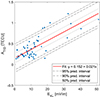 |
Figure 2 Scatter plot of the maximum TID activity index of the GNSS ground station GLSV during each one of the investigated storm events versus the maximum Kan-Lee electric field EKL in the 18 h ahead of the maximum TID activity index (Borries et al., 2023). |
For the period of 19–21 November 2003, which includes the main phase of the geomagnetic storm of November 20, 2003, for example, the following simple linear equation is obtained from the data plotted in Figure 2, y = 0.152 + 0.021x. This equation serves as the basis for estimating the ATID for this event.
Since the correlation study presented in Borries et al. (2023) was carried out by analysing the maxima values, the maximum EKL in a 2-hour interval (max2h EKL, Fig. 3b) is used to predict the ATID index. Different intervals could be used, but we have empirically chosen 2 h, aiming at maximizing the prediction performance.
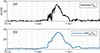 |
Figure 3 (a) EKL and (b) max2 h EKL for one day before, the day of the onset and one day after November 20, 2003 geomagnetic storm. |
The following linear regression equation derived from Figure 2 is then used for the prediction: (7)where n represents the 0, 30, 60, … 180-minute prediction time. The
  estimates are then compared with the ATID reference values at t, t + 30, …, t + 180.
This procedure is performed for each storm event. Here we have used a leave-one-out cross-validation scheme to make the predictions. In this case, assuming that the maxima from N geomagnetic storm events are available, we use the maxima from N − 1 events to generate the scatter plot and then derive the linear regression equation, which is used to predict the ATID for the Nth storm event following the procedure described before.
The results of this methodology for predicting the ATID for the November 20, 2003 geomagnetic storm can be found in Section 3.1.
2.4.2 LRNNAE
Previous investigations have shown that the Auroral Electrojet (AE) index presents a high correlation with the amplitude of LSTIDs (Borries et al., 2009, 2023). The recent study presented in Borries et al. (2023) has found a correlation coefficient of 0.72 between the maximum ATID registered at each event, and the maximum AE index registered in the 18 h prior to the occurrence of the maximum ATID. For our predictions purpose, however, instead of using the AE index, a predicted AE index is used. Although the World Data Center (WDC) for Geomagnetism Kyoto provides plots of the real-time AE index on its website, the real-time data is currently not available to the public, and the provisional data may take several days to be officially released (WDC, 2022). Therefore, to evaluate the prediction of the ATID for an operational scenario, we use the AE index derived from solar wind measurements at Lagrangian Point L1 and predicted by an NN model. The NN predicted AE (NNAE) is based on the model described in Ferreira & Borges (2021), where the AE index is predicted using the solar wind velocity, the B y and B z components of the IMF together with the day of the year and temporal information. The idea of including the NNAE index is to verify if it can provide better performance than using the EKL coupling function as input. It is important to note that the predictions of the ATID obtained by using the NNAE may differ from those that would be obtained by using the AE index.
The prediction of the ATID index is then made in a similar way to the procedure presented in Section 2.4.1. In this case, the max2h NNAE is used as the input to the model, as shown in equation (8): (8)
(8)
Figure 4 presents the maximum values of ATID and NNAE together with the linear regression equation, which is used to perform the ATID index prediction for the November 20, 2003 geomagnetic storm.
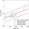 |
Figure 4 Scatter plot of the maximum TID activity index of the GNSS ground station GLSV during each of the 56 storm events versus the maximum NNAE in the 18 h ahead of the maximum TID activity index (Borries et al., 2023). |
The results of this methodology and their comparison with the other investigated methodologies are presented in Section 3.1.
2.5 Neural Network model (NN)
As an alternative to the PM and the LR models presented in the previous sections, a model based on artificial neural networks (NNs), more specifically, the multi-layer perceptron (Haykin, 2009) is proposed. Different investigations in space weather and ionospheric research have shown that multi-layer perceptron NNs can be a useful tool for prediction tasks (Orus-Perez, 2018; Camporeale, 2019). These networks are based on single units called neurons, which can be represented as (9)where a is the output of the neuron; g is the activation function, which is usually a non-linear function such as hyperbolic tangent or rectified linear unit (ReLu); W
x
is the synaptic weight of the neuron; X is the input value; and b is a bias term (Haykin, 2009; Orus-Perez, 2018). These neurons are massively interconnected and the network can be structured in various layers. The network can then be trained iteratively using input–output pairs.
(9)where a is the output of the neuron; g is the activation function, which is usually a non-linear function such as hyperbolic tangent or rectified linear unit (ReLu); W
x
is the synaptic weight of the neuron; X is the input value; and b is a bias term (Haykin, 2009; Orus-Perez, 2018). These neurons are massively interconnected and the network can be structured in various layers. The network can then be trained iteratively using input–output pairs.
The NN model proposed in this work was implemented based on the TensorFlow open source library1 and takes as inputs the Solar Zenith Angle (SZA), to account for the daily variability observed in the LSTIDs activity described in Borries et al. (2009), and the historical values of ATID and E KL . An illustrative schematic of the NN used in this work to predict the ATID is presented in Figure 5.
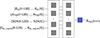 |
Figure 5 Schematic representation of the NN Model used on the ATID index prediction. |
The NN model proposed in this work consists of one input layer, one output layer and two hidden layers of neurons. For the hidden layers, the ReLu activation function was used and a linear activation function was used in the output layer. The network was trained with 600 epochs, a learning rate of 1.5 × 10⁻⁴ and a batch size equal to 2048, and the training/validation procedure was performed using the leave-one-out cross-validation scheme in the same way as presented in Section 2.4. In this case, the performance of the model is tested for all available events, which differs from the procedure presented in Kim et al. (2021), which presents the prediction of the ionospheric state during geomagnetic storms using LSTM neural networks. In that study, from a set of 70 geomagnetic storms, 60 events are selected for training, 7 events for validation and 3 events for testing. Since in the proposed approach the model is tested in all events, it may provide a more comprehensive assessment of the model’s performance during different parts of the solar cycle and for storms with different characteristics.
The results of the NN model and the comparison with the other proposed methodologies are presented and discussed in the following sections.
3 Results
This section presents the evaluation results for each one of the proposed models, taking into consideration 56 geomagnetic storm events observed from 2001 to 2017. The storms from 2001 to 2007 were selected based on the list of geomagnetic storms presented in Borries et al. (2009). In addition, geomagnetic storm events from 2008 to 2017 have been included based on SYM-H index values below −50 nT. For each geomagnetic storm event, 3 days are usually included in the analysis: the day on which the SYM-H index reached the minimum value, and the days before and after. It is important to highlight that the list of selected events presented in Appendix does not include all geomagnetic storm events with SYM-H index values below −50 nT in the period from 2001 to 2017. Geomagnetic storm events with missing or significant gaps in GNSS data, AE index and solar wind measurements were not included in the analysis. Similarly to the investigation presented in Borries et al. (2023), the geomagnetic storm event observed on November 20, 2003 is used to illustrate the results of each model on the prediction activity.
Figures 6a and 6c show the results of the 1-hour prediction using the LR models. The ATID computed for the GLSV station during this event reached magnitudes of about 0.8 TECU, indicating a moderate/strong TID activity over the station. During this period one can observe that both proposed LR based methodologies were able to clearly reproduce the increase of the ATID. However, the rapid fluctuations in the ATID are not well reproduced by the models.
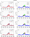 |
Figure 6 Left panels: One-hour prediction of the TID activity index during the geomagnetic storm event registered on the 20th of November 2003 using: (a) LREKL, (c) LRAE, (e) PM and (g) NN model. Right panels: The same predictions presented in the left panel, but evaluated as a classification problem, showing True Positives (TP), True Negatives (TN), False Positives (FP) and False Negatives (FN) for a threshold of 0.5 TECU obtained using: (b) LREKL, (d) LRAE, (f) PM and (h) NN model. |
Figure 6e shows the prediction results obtained from the PM and Figure 6g the results of the NN model described in Section 2.5. It can be observed that the NN model also clearly reproduces the ATID increase. Similar to the results obtained with the LREKL and LRAE models, one can observe that the NN model also overestimated the ATID index in the early morning of November 21, 2023. The right column of Figure 6 presents the results of the model when it is evaluated from the perspective of a classification problem, which is described in the following section.
3.1 LSTID activity detection performance
As presented in Figure 6, all the proposed methodologies are able to predict fairly well the ATID index increases observed during the storm. The rapid fluctuations observed in the ATID index are, on the other hand, not very well depicted by the methodologies. Similar to what is presented in Borries et al. (2023), the models are evaluated from the perspective of a classification task. According to this approach, any predicted value of ATID greater than or equal to the threshold level is considered as an LSTID activity event and a predicted value below this threshold is considered as a non-LSTID activity event. This type of classification leads to the possibilities of True Positive (TP, when both the reference and predicted values are above the threshold), True Negative (TN, when both the reference and predicted values are below the threshold), False Positive (FP, when the reference value is below the threshold, but the predicted value is above the threshold) and False Negative (FN, when the reference value is above the threshold, but the predicted value is below the threshold) by comparing the reference and estimated values (Borries et al., 2023). Figure 6 (right panels) shows the predictions of the proposed models, based on this classification methodology. Here the chosen threshold to identify the occurrence or not of LSTIDs is equal to 0.5 TECU, which corresponds to the 98% percentile of the ATID considering all values and events. One can observe that all methodologies present good estimates of TNs and different performances in the identification of TPs. In this specific case, one can note that the LREKL present the best performance in the detection of TP values.
The metric used in the evaluation of the predictions is the True Skill Statistic (TSS), which is computed based on the difference between the True Positive Rate (TPR) and the False Positive Rate (FPR). The latter corresponds to the probability of false alarm and is computed as the ratio of False Positives to the number of negative events (N). The former indicates the ability to find all positive events and corresponds to the ratio of true positives to all positive events (P), as shown in equation (10). (10)
(10)
The TSS has the advantage of being unbiased with respect to class imbalance (Detman & Joselyn, 1999; Camporeale, 2019; Borries et al., 2023). It ranges from −1 to 1, where −1 is interpreted as always wrong predictions (Bobra & Couvidat, 2015), 0 or less mean no better than random performance (Detman & Joselyn, 1999) and 1 means perfect forecasts. The TSS is obtained by considering the predictions of all the investigated events for the different models and different prediction times, which vary from 0 to 180 min. Figure 7a shows the TSS obtained by each model considering the different lead times for prediction.
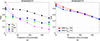 |
Figure 7 (a) TSS for the different models under investigation, i.e. regression (obtained from EKL and AE), NN and the PM and (b) the TSS obtained from the combination of some of such models using a weighted average scheme. |
As expected, for nowcast activities, the PM reaches the maximum achievable TSS of 1, since it is identical to the ground truth. For longer prediction times, one can observe that the TSS for the PM significantly drops when increasing the leading time of prediction, reaching about 0.15 for 180-minute predictions. The other models presented lower TSS for nowcasting activities, but one can notice that the reduction in performance with the increase in the leading times is not as dramatic as the one observed for the PM.
For lead times greater than 30 min, the TSS of LREKL is greater than the TSS of all the models under analysis. One can also observe that in this case the TSS peaks at 30 min (TSS = 0.8) and decreases continuously for longer lead times, reaching a TSS of 0.5 for 180 min predictions. The LRNNAE model outperforms the PM for lead times equal to or greater than 60 min, but has a lower performance when compared to the LREKL and a similar performance when compared to the NN model. It is important to highlight that the performance of the LRNNAE model is affected by the performance of the AE index prediction. The NN-based model shows an overall TSS higher than the PM and the LRNNAE for prediction lead times equal to or greater than 60 min. One can observe from Figure 7a that all proposed models presented higher TSS when compared to the baseline PM for predictions beyond 60 min.
To further investigate the performance of each model, Figure 8 shows the TPR, FPR and the TSS for a one-hour prediction. From the results, one can clearly note that all the models present low FPR, with the NN and PM models presenting the lowest levels (below 1%). The main difference in performance is led by the TPR, which is the highest for the predictions obtained from the LREKL. In this case, the observed TSS was 0.76. The other proposed models showed similar performance among them.
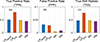 |
Figure 8 Statistics obtained from the different models for 60 min prediction: (a) True Positive Rate, (b) False Positive Rate and (c) True Skill Statistic. |
3.2 Multi-Model Ensemble (MME)
An additional methodology investigated in this work is the multi-model ensemble (MME), which corresponds to a combination of different models in order to increase the performance of a single-model prediction. The main focus here is to investigate whether such a methodology can improve the performance of the model with the highest performance obtained so far, i.e. LREKL. A basic approach is the linear combination of different methods in order to create a better ensemble forecast (Murray, 2018). Taking probability forecasts as an example, one can combine multiple forecast probabilities outputs from n different models according to Pens = ∑ n ω n p n , where p denotes a forecast probability value and ω is the weight value (often chosen in such a way that the sum of all weights equals to 1 (Murray, 2018; Zhou, 2012).
Different approaches can be used to set the weights for each model, which may go from simple ensemble averages (which tend to be used in operational forecasting methods, for example) up to nonlinear weighting schemes. Other weighting schemes based on performance metrics can be used in order to improve the forecasts based on the user-end requirements (Murray, 2018). In this work, a weighting scheme that takes into account the performance of each model in predicting the ATID at different levels is adopted. The weights were heuristically chosen in this case. The weighting procedure is performed according to equation (11)
 (11)where LREKL(t) is the prediction obtained from the LREKL model step t, and M2 (t) is the prediction obtained from one of the other models under investigation (i.e. PM or NN model). The LREKL model was included in all multi-model combinations due to its good performance when compared to the other models, in an attempt to investigate if such combinations could improve the performance of the single model. Many other approaches for assigning the weights could be adopted, such as defining the weight according to the prediction time (i.e., higher weights for PM for short-term predictions and LREKL for long-term predictions). In this work, for the sake of simplicity, we only demonstrate the performance of the approach shown in equation (11).
The TSS for the ensembles investigated in this work are presented in Figure 7b. The results indicate that the combination of the LREKL and PM models can improve by about 22% and 8% for the nowcast and 30-minute predictions, respectively, when compared to the predictions obtained by the LREKL alone. For a prediction lead time of 60 min, no significant changes were observed. Beyond this prediction horizon, the results indicate that the combination of models did not lead to an improvement in performance, but rather to a slight degradation. The ensemble of LREKL with the NN model shows an improvement in the nowcasting performance, with the performance of the combination exceeding the individual performance of either methodology. For predictions equal to or longer than 30 min, no improvement was observed, but a slight decrease in performance.
4 Discussion
The analysis presented in the previous section shows different approaches for the prediction of LSTID activities, which were based on linear regression, neural networks and multi-model ensembles. The methodologies are based on the use of solar wind data from the Lagrangian point L1 to predict the level of TID activity. The model proposed by Borries et al. (2023), which is based on a linear regression with the EKL as input, has already shown good performance in predicting the ATID index. By considering the solar wind propagation time from L1 to the Earth’s bow shock, an immediate impact of the solar wind on the TID generation and the time taken by the LSTID to travel from the border of the auroral oval to the mid-latitudes, one can see a good agreement with the lead times that presented good performance, confirming the applicability of the models for predicting LSTID activity moments ahead of the storm commencement. In order to further advance and in an attempt to improve such predictions, a new linear regression-based model taking the NNAE index as input has been investigated. The results obtained have shown that the performance of the LRNNAE has not surpassed the performance of the LREKL in any of the prediction horizons investigated, which suggests that, although it outperforms the baseline model (PM) for predictions beyond 60 min, the NNAE is not an optimal parameter for estimating the LSTIDs activity index via LR.
By analysing the performance of the NN model presented in Figure 7a, one can note that, except for nowcasting purposes, no improvement was observed when using a more complex model to predict the ATID index. For predictions beyond 60 min, the NN model outperforms the PM model and has a similar performance to the LRNNAE model, but the model presents a performance of 35% lower than LREKL on average. These results, although unexpected at first glance given the recent successes reported for the use of machine learning algorithms in various applications, represent a good opportunity to discuss the idiosyncrasies and challenges of the machine learning methods that have to be carefully considered when using such a methodology. Such features may include data quality, over/underfitting, network topology, training/validation, testing and metric methodologies (Camporeale, 2019). In this case study, although a larger number of geomagnetic storms were registered from 2001 to 2017, a limited amount of geomagnetic storms was used to develop and test the model. Several geomagnetic storm events were removed from the analysis, due to the occurrence of data gaps, either in solar wind data, geomagnetic data (AE index) or GNSS data, which limits the amount of representative data to be used to train the NN model. In addition, each one of the observed geomagnetic storm events has its own features in terms of time of occurrence, background ionization levels, and coupling from below, for example. As reported by Camporeale (2019), the too often too quiet problem makes the space weather datasets quite unbalanced, which poses a serious challenge to any machine learning algorithm trying to find patterns in the data. Such complexity summed up with a reduced dataset and high diversity of the geomagnetic events, poses a challenge for the prediction using the proposed NN model. Similar reduced performance of artificial neural network models when compared to simple methodologies has been already observed in other investigations, such as Reikard (2018), where logistic regression consistently outperformed the artificial neural network in predicting solar irradiance, sunspot number, and the Aa and Am geomagnetic indices. Also, in some cases presented in Wrench et al. (2022), NN models performed worse than simple models (e.g. linear interpolation) in interpolation tasks for predicting statistics of sparse IMF data series obtained from the Parker Solar Probe. These studies evidence that a gain in performance from using such a methodology may not be always the case. However, it is important to highlight that in this study the NN model outperformed the LREKL for nowcasting and outperformed both the LRNNAE and the PM for the predictions beyond 60 min.
When comparing all the investigated models with the LREKL, one can note a clear difference in the performance. For the 1-hour predictions, the LREKL model is followed in performance by the NN, LRNNAE (both with similar performance) and PM models, respectively. Although all the models presented a low FPR, the LREKL presented the highest TPR, which in this case translated into a higher TSS. Different factors may contribute to this.A low signal-to-noise ratio summed up with a limited number of geomagnetic events poses significant challenges for the development of prediction models. Improving the data pre-processing for the generation of the ATID and increasing the database of events could be a good way to improve the preconditions for the development of the prediction models. It is important to highlight that all models presented higher performance than the baseline PM model for predictions beyond 60 min. The NN model (described in Sect. 2.5) presented better results than almost all the other models for predictions beyond 60 min. Its lower performance when compared to the LREKL, however, may be attributed to the higher level of underestimation in this model when higher levels of ATID are observed, which leads to a decrease in TPR. One of the possible causes for the underestimation could be the scarce dataset showing a low number of storms with significantly high ATID values, which could then affect the NN estimates. Also, due to the different characteristics and features of each geomagnetic storm event, the amount of geomagnetic storm events used to train the model may not be representative enough. The MMEs did not significantly improve the prediction results beyond 60 min. However, improvements were observed for prediction lead times shorter than 60 min, which suggests that the combination of the LREKL and the PM could be a useful solution for short-term predictions/nowcasting of the LSTID activity level.
4.1 Longitudinal variability
As presented in the previous sections, the analysis has so far been performed considering the GLSV station only. In order to investigate whether there is a difference in performance for different longitudinal sectors, we include the stations BOR1, HERS, and NVSK in the analysis, whose locations are presented in Figure 9.
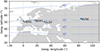 |
Figure 9 Location of the GLSV, BOR1, HERS and NVSK GNSS stations. Geomagnetic latitudes of 30, 40, 50 and 70° N of are indicated by the dashed blue lines. |
Given the better performance of the LREKL model presented for the GLSV station, we have selected this model to investigate how it performs for the other stations located at a similar geomagnetic latitude. The prediction performance is illustrated for the November 20, 2003 geomagnetic storm, and more than 50 storms are used to obtain the regression lines, which are shown in Figure 10a for this geomagnetic storm. The complete list of storms used in this analysis is presented in Appendix. In this case, we again use a leave-one-out approach to test the model. With this approach, the model is tested for predicting the ATID index for more than 50 stations, and the results are summarized in the TSS plots for each station in Figure 10c. Similar to what was observed for GLSV, the ATID predicted by the LREKL reflects the increase in the reference ATID observed during the storm. The TSS considering all the storms for each station is quite similar to the results obtained for the GLSV station.
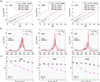 |
Figure 10 (a) Regression lines for predicting ATID index for the November 20, 2003 geomagnetic storm, (b) prediction of the ATID index for the November 20, 2003 geomagnetic storm and TSS (c) for the BOR1, HERS and NVSK stations obtained after evaluating the model on the storms described in the Appendix. |
5 Conclusions
In this study, we investigated the performance of different methodologies in predicting the LSTIDs activity via the ATID index, which is a useful index developed for statistical analysis of TIDs activity. The set of models investigated in this work includes: two models based on linear regression (LREKL and LRNNAE), a neural network-based model ( ), and the persistence model (PM), which is taken as the baseline model. The results show that all proposed models outperformed the baseline model PM for predictions beyond 1 h. For 1-hour predictions, all models presented a rather low FPR, which indicates that the difference in TSS for each model is associated with the TPR in this case. The investigation of the performance for other GNSS stations (BOR1, HERS and NVSK) has shown similar results to those obtained for the GLSV station, demonstrating the capabilities of the LREKL model to predict TID activity during geomagnetic storms for other longitudes at mid-latitudes in the European region. As already presented, the main goal of this study is to understand if and how much other state-of-the-art methodologies can improve the linear regression-based methodology for predicting the ATID index at mid-latitude Europe during geomagnetic storms presented in Borries et al. (2023). The results have shown that more complex models do not necessarily lead to an increase in performance, as may be sometimes expected. For the GLSV station, the LREKL model outperformed the NN model in almost all lead times of prediction. Although the NN model provides the lowest FPR, the TSS obtained with this methodology could not surpass the TSS of the LREKL, except for nowcast activities.
It is important to note that although the results of the NN model for this particular study did not outperform the LREKL, it performed similarly to the LRNNAE and better than the PM for predictions beyond one hour. This suggests that the NN model should not be completely discarded, but could also be improved in terms of hyperparameters optimization, number of neurons and layers, and selection of input parameters. In addition, the quality of the dataset in terms of coverage, noise, and cause-effect relationship has to be carefully taken into consideration when using such a methodology. The study also showed that multi-model ensembles may be a good alternative to improve the estimates of different models. Even the combination of simple models (LREKL and PM) led to an increase in performance for short-term predictions. In this specific case, this methodology provided a good improvement in performance for 30-minute prediction. The recent developments in machine learning algorithms and multi-model ensembles provide new possibilities for space weather prediction and modelling applications, and different investigations have shown their advantages and limitations. The already established simple methodologies, should not be disregarded and can, depending on the situation, still be considered powerful tools for approaching complex problems.
Acknowledgments
For generating the TID activity index, we used RINEX files from IGS for the dates before 2015 and processed line of sight TEC data from Madrigal database. For predicting the AE index, we used ACE solar wind data from ACE-MAG, ACE-SWICS and ACE-SWEPAM instruments www.srl.caltech.edu/ACE/ASC/level2/, and the auroral electrojet indices AE from https://wdc.kugi.kyoto-u.ac.jp/aeasy/index.html. The data is publicly available and we like to thank the data providers for sharing their data. The authors would like to thank the Brazilian agencies Federal District Research Support Foundation (FAPDF) and the National Council for Scientific and Technological Development (CNPq) that partially supported this work. The editor thanks three anonymous reviewers for their assistance in evaluating this paper.
References
- Aa E, Zou S, Ridley A, Zhang S, Coster AJ, Erickson EJ, Liu S, Ren J. 2019. Merging of storm time midlatitude traveling ionospheric disturbances and equatorial plasma bubbles. Space Weather 17: 1–14. https://doi.org/10.1029/2018SW002101. [CrossRef] [Google Scholar]
- Becker-Guedes F, Sahai Y, Fagundes PR, Espinoza ES, Pillat VG, et al. 2007. The ionospheric response in the Brazilian sector during the supergeomagnetic storm on 20 November 2003. Ann Geophys 25: 863–873. https://doi.org/10.5194/angeo-25-863-2007. [CrossRef] [Google Scholar]
- Bobra MG, Couvidat S. 2015. Solar flare prediction using SDO/HMI vector magnetic field data with a machine-learning algorithm. Astrophys J 798(2): 135. https://doi.org/10.1088/0004-637X/798/2/135. [Google Scholar]
- Borries C, Ferreira AA, Nykiel G, Borges RA. 2023. A new index for statistical analyses and prediction of traveling ionospheric disturbances. J Atmos Sol-Terr Phys 247(106069): 1–13. https://doi.org/10.1016/j.jastp.2023.106069. [CrossRef] [Google Scholar]
- Borries C, Jakowski N, Kauristie K, Amm O, Mielich J, Kouba D. 2017. On the dynamics of large-scale traveling ionospheric disturbances over Europe on 20 November 2003. J Geophys Res Space Phys 122(1): 1199–1211. https://doi.org/10.1002/2016JA023050. [CrossRef] [Google Scholar]
- Borries C, Jakowski N, Wilken V. 2009. Storm induced large scale TIDs observed in GPS derived TEC. Ann Geophys 27: 1605–1612. https://doi.org/10.5194/angeo-27-1605-2009. [CrossRef] [Google Scholar]
- Bukowski A, Ridley A, Huba JD, Valladares C, Anderson PC. 2024. Investigation of large scale traveling atmospheric/ionospheric disturbances using the Coupled SAMI3 and GITM Models. Geophys Res Lett 51(e2023GL106015): 1–10. https://doi.org/10.1029/2023GL106015. [CrossRef] [Google Scholar]
- Buonsanto MJ. 1999. Ionospheric Storms – a review. Space Sci Rev 88: 563–601. https://doi.org/10.1023/A:1005107532631. [CrossRef] [Google Scholar]
- Camporeale E. 2019. The challenge of machine learning in space weather: nowcasting and forecasting. Space Weather 17(8): 1166–1207. https://doi.org/10.1029/2018SW002061. [CrossRef] [Google Scholar]
- Cherniak I, Zakharenkova I. 2018. Large-scale traveling ionospheric disturbances origin and propagation: case Study of the December 2015 geomagnetic storm. Space Weather 16(9): 1377–1395. https://doi.org/10.1029/2018SW001869. [CrossRef] [Google Scholar]
- Codrescu MV, Codrescu SM, Fedrizzi M. 2022. Storm time neutral density assimilation in the thermosphere ionosphere with TIDA. J Space Weather Space Clim 12(13): 1–13. https://doi.org/10.1051/swsc/2022011. [CrossRef] [EDP Sciences] [Google Scholar]
- Crowley G, Hackert CL, Meier RR, Strickland DJ, Paxton LJ, et al. 2006. Global thermosphere-ionosphere response to onset of 20 November 2003 magnetic storm. J Geophys Res 111(A10S18): 1–9. https://doi.org/10.1029/2005JA011518. [Google Scholar]
- Detman T, Joselyn J. 1999. Real-time Kp predictions from ACE real time solar wind. AIP Conf Proc 471(1): 729–732. https://doi.org/10.1063/1.58720. [CrossRef] [Google Scholar]
- Devos A, Verbeeck C, Robbrecht E. 2014. Verification of space weather forecasting at the Regional Warning Center in Belgium. J Space Weather Space Clim 4(A29): 1–15. https://doi.org/10.1051/swsc/2014025. [CrossRef] [EDP Sciences] [Google Scholar]
- Fedorenko YP, Tyrnov OF, Fedorenko VN, Dorohov VL. 2013. Model of traveling ionospheric disturbances. J Space Weather Space Clim 3(A30): 1–28. https://doi.org/10.1051/swsc/2013052. [Google Scholar]
- Ferreira AA, Borges RA. 2021. Performance analysis of distinct feed-forward neural networks structures on the AE index prediction. In: Proceedings of the IEEE Aerospace Conference 2021. IEEE, pp. 1–7. https://doi.org/10.1109/AERO50100.2021.9438504. [Google Scholar]
- Francis SH. 1975. Global propagation of atmospheric gravity waves: A review. J Atmos Terr Phys 37: 1011–1054. https://doi.org/10.1016/0021-9169(75)90012-4. [CrossRef] [Google Scholar]
- Fuller-Rowell TJ, Codrescu M. 1996. On the seasonal response of the thermosphere and ionosphere to geomagnetic storms. J Geophys Res 101(A2): 2343–2353. https://doi.org/10.1029/93JA02015. [CrossRef] [Google Scholar]
- Haykin S. 2009. Neural networks and learning machines, 3rd edn. Pearson, New Jersey, USA. [Google Scholar]
- Hernández-Pajares M, Juan JM, Sanz J. 2006. Medium-scale traveling ionospheric disturbances affecting GPS measurements:Spatial and temporal analysis. J Geophys Res 111(A07S11): 1–13. https://doi.org/10.1029/2005JA011474. [Google Scholar]
- Hines CO. 1960. Internal atmospheric gravity waves at ionospheric heights. Canadian J Phys 38: 1441–1481. https://doi.org/10.1139/p60-150. https://cdnsciencepub.com/doi/10.1139/p60-150. [CrossRef] [Google Scholar]
- Hocke K, Schlegel K. 1996. A review of atmospheric gravity waves and travelling ionospheric disturbances: 1982–1995. Ann Geophys 14: 917–940. https://doi.org/10.1007/s00585-996-0917-6. [Google Scholar]
- Hoque MM, Jakowski N. 2012. Ionospheric propagation effects on GNSS signals and new correction approaches (chap. 16.). In: Global Navigation Satellite Systems, Jin S (Ed.), IntechOpen, Rijeka. https://doi.org/10.5772/30090. [Google Scholar]
- Hunsucker RD. 1982. Atmospheric gravity waves generated in the high-latitude ionosphere: A review. Rev Geophys 20(2): 239–315. https://doi.org/10.1029/RG020i002p00293. [CrossRef] [Google Scholar]
- Jonah OF, Zhang S, Coster AJ, Goncharenko LP, Erickson PJ, Rideout W, de Paula ER, de Jesus R. 2020. Understanding inter-hemispheric traveling ionospheric disturbances and their mechanisms. Rem Sens 12(228): 1–25. https://doi.org/doi.org/10.3390/rs12020228. [CrossRef] [Google Scholar]
- Kim J, Kwak Y, YongHa K, Su-In M, Se-Heon J, Yun J. 2021. Potential of regional ionosphere prediction using a long short-term memory deep learning algorithm specialized for geomagnetic storm period. Space Weather 19: 1–20. https://doi.org/10.1029/2021SW002741. [Google Scholar]
- Kubota M, Shiokawa T, Ejiri MK, Otsuka Y, Ogawa T, Sakanoi T, Fukunishi H, Yamamoto M, Fukao S, Saito A. 2000. Traveling ionospheric disturbances obserived in the OI 630-nm nighthlow images over Japan by using a multi-point imager network during the FRONT campaing. Geophys Res Lett 27(24): 4037–4040. https://doi.org/10.1029/2000GL011858. [CrossRef] [Google Scholar]
- Maruyama T, Ma G, Nakamura M. 2004. Signature of TEC storm on 6 November 2001 derived from dense GPS receiver network and ionosonde chain over Japan. J Geophys Res 109(A10302): 1–11. https://doi.org/10.1029/2004JA010451. [Google Scholar]
- Mayr HG, Harris IH, Herrero FA, Spencer NW, Varosi F, Pesnell WD. 1990. Thermospheric gravity waves: obserivations and interpretation using the Tranfer Function Model (TFM). Space Sci Rev 54: 297–375. https://doi.org/10.1007/BF00177800. [Google Scholar]
- Meier RR, Crowley G, Strickland DJ, Christensen AB, Paxton LJ, Morrison D, Hackert CL. 2005. First look at the 20 November 2003 superstorm with TIMED/GUVI: Comparisons with a thermospheric global circulation model. J Geophys Res 110(A09S41): 1–15. https://doi.org/10.1029/2004JA010990. [Google Scholar]
- Mendillo M. 2006. Storms in the ionosphere: Patterns and processes for total electron content. Rev Geophys 44(4): 1–47. https://doi.org/10.1029/2005RG000193. [CrossRef] [Google Scholar]
- Millward G, Quegan S, Moffett R, Fuller-Rowell T, Rees D. 1993. A modelling study of the coupled ionospheric and thermospheric response to an enhanced high-latitude electric field event. Planet Space Sci 41(1): 45–56. https://doi.org/10.1016/0032-0633(93)90016-U. [CrossRef] [Google Scholar]
- Morgan MG, Calderón CHJ, Ballard KA. 1978. Techniques for the study of TIDs with multi-station rapid-run ionosondes. Radio Sci 13(4): 729–741. https://doi.org/10.1029/RS013i004p00729. [CrossRef] [Google Scholar]
- Munro GH. 1948. Short-period changes in the F region of the ionosphere. Nature 162: 886–887. https://doi.org/10.1038/162886a0. [CrossRef] [Google Scholar]
- Murray SA. 2018. The Importance of ensemble techniques for operational space weather forecasting. Space Weather 16(7): 777–783. https://doi.org/10.1029/2018SW001861. [CrossRef] [Google Scholar]
- Newell PT, Sotirelis T, Liou K, Meng C-I, Rich FJ. 2007. A nearly universal solar wind-magnetosphere coupling function inferred from 10 magnetospheric state variables. J Geophys Res Space Phys 112(A1): 1–16. https://doi.org/10.1029/2006JA012015. [Google Scholar]
- Orus-Perez R. 2018. Using TensorFlow-based Neural Network to estimate GNSS single frequency ionospheric delay (IONONet). Adv Space Res 63: 1607–1618. https://doi.org/10.1016/j.asr.2018.11.011. [Google Scholar]
- Otsuka Y, Shiokawa K, Ogawa T. 2004. Geomagnetic conjugate observations of medium-scale traveling ionospheric disturbances at midlatitude using all-sky airglow imagers. Geophys Res Lett 31(L15803): 1–5. https://doi.org/10.1029/2004GL020262. [Google Scholar]
- Otsuka Y, Suzuki K, Nakagawa S, Nishioka M, Shiokawa K, Tsugawa T. 2013. GPS observations of medium-scale traveling ionospheric disturbances over Europe. Ann Geophys 31: 163–172. https://doi.org/10.5194/angeo-31-163-2013. [CrossRef] [Google Scholar]
- Paulescu M, Paulescu E, Badescu V. 2021. Chapter 9 – Nowcasting solar irradiance for effective solar power plants operation and smart grid management. In: Predictive Modelling for Energy Management and Power Systems Engineering, Deo R, Samui P, Roy SS (Eds.), Elsevier, pp. 249–270. https://doi.org/10.1016/B978-0-12-817772-3.00009-4. [CrossRef] [Google Scholar]
- Prölss GW. 1980. Magnetic storm associated perturbations of the upper atmosphere: recent results obtained by satelliute-Borne Gas Analyzers. Rev Geophys Space Phys 18(1): 183–202. https://doi.org/10.1029/RG018i001p00183. [CrossRef] [Google Scholar]
- Reikard G. 2018. Forecasting space weather over short horizons: Revised and updated estimates. New Astron 62: 62–69. https://doi.org/10.1016/j.newast.2018.01.009. [CrossRef] [Google Scholar]
- Reinisch B, Galkin I, Belehaki A, Paznukhov V, Huang X, et al. 2018. Pilot ionosonde network for identification of traveling ionospheric disturbances. Radio Sci 53: 365–378. https://doi.org/10.1002/2017RS006263. [CrossRef] [Google Scholar]
- Ridley AJ, Deng Y, Tóth G. 2006. The global ionosphere-thermosphere model. J Atmos Sol-Terr Phys 68: 839–864. https://doi.org/10.1016/j.jastp.2006.01.008. [CrossRef] [Google Scholar]
- Saito A, Fukao S, Miyazaki S. 1998. High resolution mapping of TEC perturbations with the GSI GPS Network over Japan. Geophys Res Lett 25(16): 3079–3082. https://doi.org/10.1029/98GL52361. [CrossRef] [Google Scholar]
- Sheng C, Deng Y, Zhang S, Nishimura Y, Lyons LR. 2020. Relative contributions of ion convection and particle precipitation to exciting large‐scale traveling atmospheric and ionospheric disturbances. J Geophys Res Space Phys 125: 1–11. https://doi.org/10.1029/2019JA027342. [CrossRef] [Google Scholar]
- Tsugawa T, Saito A. 2004. A statistical study of large-scale traveling ionospheric disturbances using the GPS network in Japan. J Geophys Res 109(A06302): 1–11. https://doi.org/10.1029/2003JA010302. [Google Scholar]
- Vadas SL, Figueiredo C, Becker E, Huba JD, Themens DR, Hindley NP, Mrak S, Galkin I, Bossert K. 2023. Traveling ionospheric disturbances induced by the secondary gravity waves from the Tonga Eruption on 15 January 2022: Modeling with MESORAC-HIAMCM-SAMI3 and comparison with GPS/TEC and ionosonde data. J Geophys Res Space Phys 128(6): 1–33. https://doi.org/10.1029/2023JA031408. [Google Scholar]
- WDC. 2022. Version definitions of AE and Dst geomagnetic indices. Technical Report. WDC for Geomagnetism, Kyoto. Available at https://wdc.kugi.kyoto-u.ac.jp/wdc/pdf/AEDst_version_def_v2.pdf. [Google Scholar]
- Wrench D, Parashar TN, Singh RK, Frean M, Rayudu R. 2022. Exploring the potential of neural networks to predict statistics of solar wind turbulence. Space Weather 20(9): 1–16. https://doi.org/10.1029/2022SW003200. [CrossRef] [Google Scholar]
- Yokoyama T. 2014. Hemisphere-coupled modeling of nighttime medium-scaletraveling ionospheric disturbances. Adv Space Res 54: 481–488. https://doi.org/10.1016/j.asr.2013.07.048. [CrossRef] [Google Scholar]
- Zakharenkova I, Astafyeva E, Cherniak I. 2016. GPS and GLONASS observations of large-scale traveling ionospheric disturbances during the 2015 St. Patrick’s Day storm. J Geophys Res Space Phys 121(12): 12138–12156. https://doi.org/10.1002/2016JA023332. [CrossRef] [Google Scholar]
- Zhang J, Richardson G, Webb DF, Gopalswamy N, Huttunen E, et al. 2007. Solar and interplanetary sources of major geomagnetic storms (Dst ≤ −100 nT) during 1996–2005. J Geophys Res 112(A10): 1–19. https://doi.org/10.1029/2007JA012321. [Google Scholar]
- Zhou Z. 2012. Ensemble methods: Foundations and algorithms. 1st edn. Chapman & Hall/CRC Machine Learning & Pattern Recognition Series, Boca Raton, Florida. https://doi.org/10.1201/b12207. [CrossRef] [Google Scholar]
Appendix
List of geomagnetic storm events used for each GNSS station analysis. Events used for the station are indicated by the * symbol.
Cite this article as: Ferreira AA, Borries C & Borges RA. 2025. Assessment of models for the prediction of the Travelling Ionospheric Disturbance activity index in mid-latitude Europe. J. Space Weather Space Clim. 15, 20. https://doi.org/10.1051/swsc/2025014.
All Tables
List of geomagnetic storm events used for each GNSS station analysis. Events used for the station are indicated by the * symbol.
All Figures
|
Figure 1 (a) SYM-H index, (b) Bz component of the interplanetary magnetic field, (c) solar wind speed and (d) AE index for 19–21 November, 2003. |
| In the text | |
|
Figure 2 Scatter plot of the maximum TID activity index of the GNSS ground station GLSV during each one of the investigated storm events versus the maximum Kan-Lee electric field EKL in the 18 h ahead of the maximum TID activity index (Borries et al., 2023). |
| In the text | |
|
Figure 3 (a) EKL and (b) max2 h EKL for one day before, the day of the onset and one day after November 20, 2003 geomagnetic storm. |
| In the text | |
|
Figure 4 Scatter plot of the maximum TID activity index of the GNSS ground station GLSV during each of the 56 storm events versus the maximum NNAE in the 18 h ahead of the maximum TID activity index (Borries et al., 2023). |
| In the text | |
|
Figure 5 Schematic representation of the NN Model used on the ATID index prediction. |
| In the text | |
|
Figure 6 Left panels: One-hour prediction of the TID activity index during the geomagnetic storm event registered on the 20th of November 2003 using: (a) LREKL, (c) LRAE, (e) PM and (g) NN model. Right panels: The same predictions presented in the left panel, but evaluated as a classification problem, showing True Positives (TP), True Negatives (TN), False Positives (FP) and False Negatives (FN) for a threshold of 0.5 TECU obtained using: (b) LREKL, (d) LRAE, (f) PM and (h) NN model. |
| In the text | |
|
Figure 7 (a) TSS for the different models under investigation, i.e. regression (obtained from EKL and AE), NN and the PM and (b) the TSS obtained from the combination of some of such models using a weighted average scheme. |
| In the text | |
|
Figure 8 Statistics obtained from the different models for 60 min prediction: (a) True Positive Rate, (b) False Positive Rate and (c) True Skill Statistic. |
| In the text | |
|
Figure 9 Location of the GLSV, BOR1, HERS and NVSK GNSS stations. Geomagnetic latitudes of 30, 40, 50 and 70° N of are indicated by the dashed blue lines. |
| In the text | |
|
Figure 10 (a) Regression lines for predicting ATID index for the November 20, 2003 geomagnetic storm, (b) prediction of the ATID index for the November 20, 2003 geomagnetic storm and TSS (c) for the BOR1, HERS and NVSK stations obtained after evaluating the model on the storms described in the Appendix. |
| In the text | |
Current usage metrics show cumulative count of Article Views (full-text article views including HTML views, PDF and ePub downloads, according to the available data) and Abstracts Views on Vision4Press platform.
Data correspond to usage on the plateform after 2015. The current usage metrics is available 48-96 hours after online publication and is updated daily on week days.
Initial download of the metrics may take a while.