| Issue |
J. Space Weather Space Clim.
Volume 15, 2025
Topical Issue - Fast and slow solar winds: Origin, evolution and Space Weather effects
|
|
|---|---|---|
| Article Number | 32 | |
| Number of page(s) | 12 | |
| DOI | https://doi.org/10.1051/swsc/2025027 | |
| Published online | 31 July 2025 | |
Research Article
Statistical analysis of interplanetary shock waves measured by a Solar Wind Analyzer and a magnetometer onboard the Solar Orbiter mission in 2023
1
Institute of Radio Astronomy of the National Academy of Sciences of Ukraine, Mystetstv Street, 4, Kharkiv, 61002, Ukraine
2
Space Research Centre of the Polish Academy of Sciences, Bartycka Street, 18A, Warsaw, 00-716, Poland
* Corresponding author: This email address is being protected from spambots. You need JavaScript enabled to view it.
Received:
5
December
2024
Accepted:
19
June
2025
Abstract
Interplanetary (IP) shock waves are greatly interesting, as they represent significant phenomena in near-Earth space and are direct drivers of geomagnetic and radiation storms. Moreover, various data and parameters are being explored for the identification and characterization of these waves. The spatial dimensions of shock waves vary significantly with the conditions and parameters of the propagating medium. For example, the radii of curvature of the shock wave fronts can vary by several hundred Earth radii or more in the inner heliosphere. In this study, we improved the semi-automated identification of shock waves by analyzing the solar wind and IP magnetic field (MF) parameters. More precisely, we analyzed the data recorded by the Proton Alpha Sensor of the Solar Wind Analyzer (SWA-PAS) and magnetometer (MAG) onboard the Solar Orbiter (SolO) mission. These data were collected and analyzed during the SolO journey around the Sun in 2023 at distances of 0.29–0.95 AU. Employing the developed algorithm, we identified over 40 IP-shock waves that occurred in 2023 using SWA-PAS and MAG. Additionally, we determined and presented a list of shock types and their basic parameters, kinetic and magnetohydrodynamic. The compression ratios, plasma beta βus, angle between the shock normal and upstream MF (θBn), Mach number, and others were among these parameters. Furthermore, we investigated the statistical distributions of the θBn and βus parameters in the upstream region. Finally, the dependence of the number of the identified shock waves as a function of the distance away from the Sun was explored; the number of shocks increased gradually with the increasing heliocentric distance.
Key words: Coronal mass ejection / Interplanetary shock wave / Solar wind / Space weather / Solar Orbiter
© O. Yakovlev et al., Published by EDP Sciences 2025
 This is an Open Access article distributed under the terms of the Creative Commons Attribution License (https://creativecommons.org/licenses/by/4.0), which permits unrestricted use, distribution, and reproduction in any medium, provided the original work is properly cited.
1 Introduction
Coronal mass ejections (CMEs) refer to the significant release of plasma and magnetic fields (MFs, B) from the solar corona, accompanied by various physical effects as well as alterations of the surrounding plasma environments (Hansen et al., 1971). Particularly, CMEs generate interplanetary (IP) shock waves and accelerate the transition of particles to higher energies (Gopalswamy, 2006; Yang et al., 2024). IP shocks are common events in the circumsolar space, occurring when the CME-driven solar wind (SW) speed exceeds the sonic speed (Marcowith et al., 2016). Shock waves can also be caused by processes occurring in the corotating interaction regions (CIRs) and streaming interaction regions (SIRs) (Gosling & Pizzo, 1999).
Numerous studies have demonstrated IP shocks as sudden transitions between supersonic (upstream) and subsonic (downstream) flow, marked by abrupt changes in the plasma speed (V), density (N), pressure (P), temperature (T), and MF (B) (Trotta et al., 2024b). These changes reflect the possibility of identifying the features of IP shocks, classifying them, and studying their propagation through SW (Baumjohann & Treumann, 1997). Particularly, these shocks were classified as forward/reverse shocks if they were propagating antisunward/sunward in the shock frame of reference (Burlaga, 1971). Moreover, fast forward (FF) shocks (Echer et al., 2011) are characterized by increased V, N, P, and B, whereas fast reverse (FR) shocks (Kilpua et al., 2015) are characterized by the overall decrease in all the parameters except V. Additionally, slow forward (SF) shocks are characterized by increased N, P, and V as well as decreased B. Finally, slow reverse (SR) shocks are characterized by N and P as well as increased B and V (Tsurutani et al., 2010; Kilpua et al., 2015; Oliveira & Ngwira, 2017).
Additionally, the nature of a shock wave is characterized by a set of parameters, such as the shock normal n (the perpendicular direction to the shock front), the angle between n and the upstream B (θBn), the Mach numbers (M; typically the Alfvenic M (MA) and fast magnetosonic mode M (Mfms)), and the plasma beta (β).
Furthermore, quasiparallel and quasiperpendicular shocks represent two distinct collisionless-shock types in space plasmas, particularly from the viewpoint of SW interacting with planetary magnetospheres and IP MFs (IMFs). These shocks are classified based on the θBn parameter. A quasiparallel shock occurs when θBn between the B vector and n is <45°. Put differently, it occurs when B is almost parallel to the shock-propagation direction. A quasiperpendicular shock occurs when θBn between B and n is >45°. In this case, B is almost perpendicular to the shock-propagation direction, assuming the shocks are planar.
Comprehensive studies based on observational data from various space missions (e.g., Wind, ACE, Ulysses, and Helios), supported by sophisticated analytical and numerical techniques, have been conducted to further elucidate the nature and effects of IP shocks as well as their dependence on solar activities (Kruparova et al., 2013; Kilpua et al., 2015). Numerous studies have attempted to adequately identify collisionless-shock crossings in spacecraft data. Thus, manual and automated algorithms, including machine learning (ML) approaches, have been developed for shock detection, and shock databases have been compiled for various spacecraft (Kruparova et al., 2013; Lalti et al., 2022; Oliveira, 2023).
Particularly, Kruparova et al. (2013) developed a method for detecting IP shock crossings using ion moments and B magnitudes. Thereafter, the author verified the method using Wind (at 1 AU) and Helios (at distances of 0.29–1 AU) data. The method comprised an automated two-step detection algorithm with systematically proposed quality factors (QFs) and thresholds for SW parameters. Further, Cash et al. (2014) developed an automatic IP shock detection method using eight years of ACE data to improve space weather forecasting capabilities. Notably, the heliospheric shock waves database (https://www.ipshocks.fi) is maintained by the University of Helsinki. This comprehensive database, which contains over 2900 fast shocks, was compiled through systematic visual inspection and ML techniques using data obtained from several missions.
The recently launched Solar Orbiter (SolO) mission (Müller et al., 2020), which provides high-resolution data on the plasma, B, and energetic particle parameters, is a crucial contributor to IP shock studies (Dimmock et al., 2023; Trotta et al., 2023, 2024a,b). SolO enables the detection of IP shock waves at distances of 0.28–0.95 AU, with a planned maximum inclination angle of ~24°.
Following its launch in 2020, SolO has already encountered numerous heliospheric shock waves. For instance, Trotta et al. (2023) analyzed the SolO shock observed on October 30, 2021, at 22:02:07 UT at a heliocentric distance of ~0.8 AU. The shock was a high-M IP shock with irregular “injections” of suprathermal particles generated by shock-front irregularities. The authors considered this shock an excellent avenue for studying irregular particle acceleration from a thermal plasma.
Trotta et al. (2024a) systematically studied an observed CME-driven IP shock using the Parker Solar Probe at very small heliocentric distances (0.07 AU). CME was subsequently observed by SolO on September 6, 2022, at 10:00:51 UT at a heliocentric distance of 0.7 AU. The author revealed a very structured shock transition populated by shock-accelerated protons reaching approximately 2 MeV and exhibiting irregularities in the shock downstream, which correlated with the SW structures propagating across the shock. Furthermore, Trotta et al. (2024a) emphasized that the local features of the IP shocks and their environments can vary significantly as they propagate through the heliosphere.
Most of the IP shock waves identified so far from the SolO data and studied systematically in the literature were observed between 2021 and 2022. Increased solar activity is anticipated as we approach the peak of solar cycle 25, and the observations in the coming years are expected to exhibit increased numbers of shocks detected by SolO. The solar cycle 25 Shocks Catalog, which was prepared in the frame of the EU Horyzon 2020 Serpentine Project (https://data.serpentine-h2020.eu) and recently published (Trotta et al., 2024b, 2025), probably confirmed this. Conversely, identifying shocks in more complex SW states may be more challenging, although it is crucial, especially in the context of timely space weather forecasting as well as elucidating the evolution and dynamics of collisionless shocks.
Therefore, in this study, we adapted and applied Kruparova et al. (2013) algorithm for the detection of IP shock waves collected in the SolO data between January and December 2023 at a wide range of distances away from the Sun. Specifically, we proposed new thresholds and QFs for the explored plasma and B parameters. Next, we systematically characterized the identified IP shocks based on a set of parameters and statistical studies, as well as the dependencies of the shocks on distances, along with the key information related to each shock.
Our data and methodology are presented in Section 2, and the results are presented and discussed in Section 3. Finally, the conclusions drawn from the study are summarized in Section 4. Additionally, a full list of the shock waves and their parameters are presented in Appendices A and B.
2 Materials and methods
2.1 Solar Orbiter instruments and the data for analyzing the solar wind and interplanetary magnetic field parameters
The data recorded by the Proton Alpha Sensor of the Solar Wind Analyzer (SWA-PAS) and the magnetometer (MAG) aboard the SolO mission were used to study SW and IMF parameters.
During the exploration period (January 1 to December 31, 2023), the SolO spacecraft completed two full orbits around the Sun, and the radial distance (Rd) from the Sun varied from 0.29 to 0.95 AU.
Notably, SWA-PAS is an electrostatic particle analyzer (Owen et al., 2020) that is designed to continuously measure the three-dimensional velocity-distribution function (3D-VDF) of the proton and alpha-particles as well as other parameters in the energy range of 200 eV–20 keV, divided into 96 energy intervals. The azimuth view of the space was performed using 11 separate detectors and ranges of −24° to +42°. The scanning of space by the elevation angle proceeded in the ±20° range, divided into nine sections. The energy adjustment and elevation-angle scanning were controlled by the electrostatic deflection system. Further, 3D-VDF of the SW protons and alpha-particle stream measurements were received every 4 or 300 s in the normal or fast mode at frequencies of 4–20 Hz, with decreasing measurement steps. The initial 3D-VDF data were processed by the SolO ground-tracking team and provided as the following SW parameters: N (part/cm3), velocity (V, km/s), P (j/cm3), and T (eV). In this analysis, we utilized the L2 data in the SolO RTN-coordinate reference frame with a temporal resolution of 4 s.
The IMF parameters were measured by MAG (Horbury et al., 2020) at four amplitude ranges between ±128 and ±60,000 nT, with accuracy varying from 4 to 1800 nT depending on the selected range. The cadence of the B measurements was determined by the selected mode; it was 1, 8, or 16 vectors per second in the normal mode and 64 or 128 vectors per second in the fast mode. For the analysis, we used the L2-level data of the IMF BR, BT, and BN components in the SolO RTN coordinate reference frame. The IMF measurements were conducted in the ±128 nT range with an accuracy of 4 nT at an acquisition rate of 8 vectors per second (measurements were performed every 0.125 s).
During the detailed examination of the L2-level measurement data, we observed that the time resolution of each deployed instrument varied throughout 2023. Therefore, to realize a unified time resolution for the data, we employed the linear interpolation method, with reference to the SWA-PAS time scale of 4 s.
2.2 Methodology for identifying interplanetary shock waves
Shock wave occurrences were detected via mathematical analyses and event-signature recognition. The algorithms, which were developed, based on the results of the statistical analysis of the shock wave parameters, were used to calculate the ranges of the changes in N, V, and T of SW as well as the IMF magnitude to establish the criteria under which an event can be identified as a shock wave. Studies are ongoing to obtain a sufficient set of parameters for identifying shock waves and to determine more advanced criteria for recording them. Moreover, this study is aimed at determining a relevant time for averaging the calculations. Shock-wave-recognition algorithms are subjected to constant modifications to optimize the shock-wave detection criteria and increase the reliability of space-weather forecasting.
In the frame of this study, Kruparova et al. (2013) algorithm and selection criteria were adopted for the identification of IP shock waves in the SolO-recorded data. The specified algorithm was developed for the real-time recording of shock waves regardless of their type. This algorithm was adapted when developing the operation algorithm for the Selected Burst Mode 1 trigger mode of the SolO mission. The algorithm was tested via solar wind measurements over 8 years (Wilson et al., 2021). The algorithm was based on the comparison of the steps in the changes in the N, V, and IMF magnitudes with the threshold values. QFs of the registered event considered the entire contribution of the parameter steps in the assessment of the possibility of candidates making it into a shock wave list. QF must also exceed a certain threshold value. The additional criteria defined for the values of the parameter steps enabled the exclusion of weak events. The result of the algorithm (Kruparova et al., 2013) showed that the Quality Factor (QF1) threshold was exceeded by 64%, QF2 threshold was exceeded by 29% of the total number of events considered, which were subsequently considered as candidates for IP shock.
In this study, we enhanced a semi-automatic shock wave identification algorithm incorporating the simultaneous grouped changes in N, V, and IMF. The criteria for recording the shock waves based on the statistical analysis of the data derived from the SolO Mission in 2023 were refined. Moreover, the algorithm allowed for the calculation of the main parameters of the shock waves: the B- and N-compression values, QFs, the angle between the n and B vectors, the β parameter, and the determination of the type of shock wave as well as its local direction.
As a first step, we inspected and selected the candidates after viewing the daily charts of the SW and IMF parameters throughout 2023.
Regarding the selected candidates, the relative changes in N (∆N), V (∆V), and ∆B at the first algorithm stage were calculated throughout the measurement interval (Δt), a duration of 300 s (Kruparova et al., 2013). The calculations were conducted in a day, and the beginning of Δt shifted from the beginning to the end of the day. The values of the relative changes in the parameters in the measuring interval were determined as follows:
 (1)
(1)
 (2)
(2)
 (3)
(3)
where the variables with indexes 1 and 2 correspond to the parameters at the beginning and end of Δt, respectively. The values of the relative changes in the parameters were calculated for each measurement time t.
Next, the obtained values of the relative changes in the selected parameters for SW and IMF were averaged throughout Δt, which preceded the current moment of t, and during Δt after the current moment of t. The averaged values of the parameters were designated as ΔB, ΔN, and ΔV.
At a further stage, the QFs (QF1 and QF2) were determined, following Kruparova et al.’s (2013) method. The QF values were calculated as follows:
 (4)
(4)
 (5)
(5)
Another condition for identifying an event as a real shock wave was the selection of only candidates with events whose QF1 and QF2 exceeded a certain threshold. In turn, the threshold value of QFs was selected based on the analysis of the dependence of the shock wave counts on the QF value.
3 Results and discussions
3.1 Selection of interplanetary shock waves from the candidates
While SW parameters were analyzed for the period considered, more than 50 candidates of the IP shock wave events were selected, for which simultaneous abrupt changes of the ΔN, ΔV, and ΔB values occurred. The distributions of shock candidate events as functions of ΔN, ΔV, and ΔB were calculated based on their step changes equal to 0.05.
The obtained distributions showed that most potential shocks grouped when relative changes exceeded values of 0.35 for ΔN (Fig. 1a), 0.05 for ΔV (Fig. 1b), and 0.30 for ΔB (Fig. 1c). These values were chosen as thresholds for the events to be included in the list of IP shock waves.
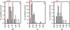 |
Figure 1 Dependence of the shock wave candidate counts (left vertical axis in all the panels) on the relative changes in the SW N, ΔN (a); V, ΔV (b); and IMF, ΔB (c). The red vertical lines represent the selected thresholds for identifying the shock waves: 0.35, 0.05, and 0.30 for ΔN, ΔV, and ΔB, respectively. |
Regarding the final inclusion of an event as a shock wave, only such events were selected from candidate events whose QF1 and QF2 exceeded the threshold value. Notably, the threshold values of QF1 and QF2 were selected based on the results of the analysis of the dependence of the shock wave candidate count on QF1 and QF2 (Fig. 2). The selected threshold values were 0.25 and 0.15 for QF1 and QF2, respectively, as the most counts of the shock wave candidates were recorded after exceeding these values.
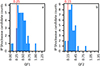 |
Figure 2 Dependence of the shock wave candidate counts (left vertical axis in all the panels) on QF1 (a) and QF2 (b). The red vertical lines represent the selected thresholds for identifying the shock waves. |
The additional conditions for including the candidates in the list of shock waves are indicated below:
event quality factor Q > QF1 or Q > QF2 (basic selection condition);
simultaneous level excesses: ΔB > 0.1, ΔN > 0.1, and ΔV > 0.03 (exclusion of events with small plasma- and IMF-parameter changes);
V1 > V2 (exclusion of events with negative ΔV).
An event was recorded as a confirmed shock wave if the event-related relative changes in all parameters simultaneously exceeded the threshold values and satisfied additional conditions. For example, Figure 3 demonstrates the visualization process for selecting doubtless shock wave candidates. Figure 3 shows a translucent red vertical strip that marks the period during which all the criteria for registering a shock wave were matched, and the red vertical dotted line shows the moment of registering the shock wave (IP Time) on 09.19.2023 at 02:22:59 UTC. Notably, IP Time was determined as the time when ΔB reached its maximum. The grey vertical translucent strip indicates the time when only some criteria were met; the event was not recorded as a shock wave.
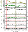 |
Figure 3 Dynamics of the SW and IMF parameters: N (a), V (b), Btot (c), ΔN (d), ΔV (e), and ΔB (f). Panels (g) and (h) display the changes in QF1 and QF2. The numerical values of the parameter thresholds are displayed in the right panels and marked by red horizontal lines. |
3.2 Basic parameters of the shock waves
Here, 44 IP shocks (40 FF, 2 FR, 1 SF, and 1 SR) were identified using the algorithm described in Sections 2 and 3.1. For comparison, the ipshocks.helsinki.fi website documented 35 shocks for SolO in 2023 (33 FF and 2 FR), whereas the publicly accessible data through the project’s Serpentine data center recorded 43 shocks (39 FF and 4 FR). The version citable through Zenodo (Trotta et al., 2024b) listed 9 shocks (all FF) for the considered period. To further characterize the registered IP shock events, a set of conventional quantitative parameters was considered. The main parameters for these events were calculated using the following widely deployed approach (e.g., Oliveira, 2023), and the values are listed in Tables A1 and B2.
Various studies have shown that the accuracy of the calculation of IP shock properties depends on the time periods upstream and downstream used for averaging SW parameters, and different approaches/time intervals have been used so far (Kilpua et al., 2015; Trotta et al., 2022; Oliveira, 2023). Specifically, Kilpua et al. (2015), using Wind data, employed an 8-minute time window for their calculations, which was based on the Helsinki database. Moreland et al. (2023), focusing on ACE measurements from 1998 to 2013, performed systematic studies on the effect of sampling windows on shock parameters, varying the time windows from 2 min to 20 min. Trotta et al. (2022), analyzing data from various space missions, considered different windows, with the smallest averaging windows being about 2 min upstream and downstream and the largest windows being about 10 min. They suggested that the extent and location of the best upstream and downstream analysis intervals vary depending on the shock.
In this work, various time windows determining the upstream (non-shocked) and downstream (shocked) periods (ranging from 5 to 10 min) were initially studied for their shock properties. Finally, the fixed and equal upstream and downstream intervals of 300 s (5 min, corresponding to 75 periods of measuring the SW parameters) were applied. These intervals were selected taking into account the shock durations, the high data resolution of the considered SolO data, the correctness of the MHD description, and, finally, their length being sufficient to average out turbulence and wave activity for as many shocks as possible.
The B and N ratios (rB and rN) were defined as the downstream mean value of the time window divided by the upstream mean value of the same time window. These ratios are expressed as follows:
 (6)and
 (7)
(7)
The upstream β (βus) parameter (the ratio of the plasma to magnetic P) was computed to characterize the upstream zone, as follows:
 (8)
(8)
where μ0 is the magnetic vacuum permeability and kB is the Boltzmann constant (e.g., Burgess, 1995; Alexandrova et al., 2007). The Alfvenic V (VA) represents another parameter in Tables A1 and B2 that depends on the B and plasma variables; this parameter was considered in the upstream region and expressed as follows:
 (9)
(9)
where mp is the proton mass.
The normal vector to the shock wave front (n), calculated using the MX3-mode method (Abraham-Shrauner & Yun, 1976; Schwartz, 1998), was subsequently applied to determine θBn, i.e., the angle between the upstream magnetic field Bus and the n vectors. Additionally, θBn controls the behavior of the particle event during the shock (Kilpua et al., 2015) and was computed as follows:
 (10)
(10)
In the next step, the shock speed, Vsh, was evaluated thus:
 (11)
(11)
The sound velocity in the IP space Cs is expressed thus:
 (12)
(12)
where the adiabatic index (γ) = 5/3 and electron temperature (Te) were calculated, following Chat et al.’s (2011) method. More specifically, the following relation for Te was used for varied SolO locations:
 (13)
(13)
where the coefficient 146,277 represents Te (in K) at 1 AU, and Rd denotes the radial distance from the Sun (in AU). The fast magnetosonic and Alfvenic Ms (Mfms and MA, respectively), as crucial characteristics of the intensity of the identified shocks, were also calculated, following Schwartz (1998):
 (14)and
 (15)
(15)
where Vfms is defined as the positive value of the expression:
 (16)
(16)
3.3 Prompt analysis of the heliocentric characteristics of the selected parameters of the shock waves
Based on the results obtained thus far, we evaluated the dependences of the N- and B-compression parameters as well as QFs as functions of the distance Rd between the SolO and Sun, and the results are shown in Figure 4.
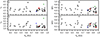 |
Figure 4 Dependences of rB (a), rN (b), QF1 (c), and QF2 (d) as functions of the distance between the SolO and Sun for each shock wave are presented in Table A1. The black points denote FF, red: FR, blue: SF, and green: SR of IP shocks. |
The obtained dependencies confirmed that the main parameters of the IP shock reached their maximum values within the measurement period at a distance of ~0.63 AU between the spacecraft and the Sun, and this is significantly associated with one specific powerful event in the IP space; thus, it was not a statistically obtained average result. The distributions of the shock wave count are determined as a function of θBn (Fig. 5a) and dependent on βus (Fig. 5b).
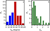 |
Figure 5 Distribution of the IPn shock counts as functions θBn (a) and βus (b). Blue bins denote IPn with θBn < 45°, while red bins correspond to θBn > 45°. |
Figure 5a shows the largest counts of the undoubted shock waves recorded at the SolO location, and it was quasiperpendicular, with an angle (θBn) of ~50°.
Figure 5a and values of θBn given in Table B2 suggest that most shock waves recorded at the SolO location in 2023 can be considered as quasiperpendicular (θBn > 45°, red bins in Fig. 5a), with the dominant number of cases around ~50°.
The histogram in Figure 5b indicates that the majority of the registered shock waves are characterized by βus values less than 1, highlighting the dominant role of the magnetic field in dynamics compared to thermal motion in these cases. The shock waves with βus > 1 were also observed in 8 out of 44 cases, but the maximum values of βus did not exceed 3.25.
3.4 Distribution of the shock waves along the Solar Orbiter trajectory
As SolO is located at various distances from the Sun at each moment, elucidating the dependence of the number and intensity of the identified shock waves on the heliocentric distance was crucial. To visualize each shock wave along the trajectory of the mission, QF1 and QF2 were deployed as indicators of the intensity of the event, as they simultaneously contain information about ΔN, ΔV, and ΔB; the elucidated dependencies are shown in Figure 6.
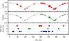 |
Figure 6 Distributions of the shock waves recorded by the SWA-PAS and MAG instruments in 2023 along the SolO trajectory compared with the X-, M-, and C-class solar flares obtained from the STIX Data Center. The dark dots in panels a and b indicate the daily average (UTC ≈ 12:00) spacecraft location according to the Solar-MACH catalog (https://solar-mach.github.io), with a time step of 1–5 days. The top panel shows the moments of registering the shock waves for QF1 in the form of spheres of different diameters; the middle panel displays the same information as Panel a, but for QF2. The diameters of the spheres were proportional to the QF1 and QF2 values listed in Table A1. Panel c shows the time points at which different-class X-ray flares were recorded. |
To explore the sources of the shock waves in the inner heliosphere, the fast coronal mass ejections (CMEs) or solar wind stream interaction regions (SIRs) must be considered. To study this relationship, we compared the time moments of solar flare occurrence (STIX Data Center)1 with the shock waves identified during the SolO travel time, and the resulting dependence is displayed in Figure 6c. The red triangles indicate the registered X-class solar flares and the M- and C-class solar flares are shown in green and blue, respectively. Here, we did not consider B-class solar flares because of their lower efficiency in producing various manifestations in the interplanetary space, including CMEs, as compared with M- and X- classes of solar flares.
The CMEs, in their turn, may produce shock waves in the interplanetary space. In summary, 16, 6, and 7 C-, M-, and X-class flares, respectively, were recorded in 2023 (STIX Data Center, DONKI Database2). Figure 6c shows that the following solar flares were recorded in a Rd of 0.55–0.65 AU: 5, 1, and 1 C-, M2.1-, and X4-class flares, respectively. We assume that these solar flares could induce local amplification in IPn and NIP_Rd in the Rd segment (Rd = 0.55…0.65 AU; Fig. 7a).
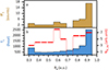 |
Figure 7 a) Dependence of the number of shock waves (IPn) as a function of Rd; b) Dependence of the time spent on passing a particular segment (length = 0.067 AU; Ts) as a function of Rd; NIP_Rd is the ratio of IPn on each segment (IPs) to Ts as a function of Rd. |
The determination of the dependence of the number of shock waves on the heliocentric distance requires the consideration of the time spent by the spacecraft on each trajectory segment to normalize the data.
We examined the distribution of the number of identified shock waves based on the distance between the Sun and the spacecraft throughout 2023. During this period, SolO completed two orbits around the Sun. Notably, the minimum and maximum Rd were 0.29 and 0.95 AU, respectively. To analyze the events, the full Rd range was divided into 10 equal segments (length = 0.067 AU). The moment at which the spacecraft entered the segment and the time spent on its passage were determined using the Solar Orbiter Archive data3, and the results are shown in Figure 7.
The dependence of NIP_Rd on the time the spacecraft passes this segment as a function of Rd (NIP_Rd) is derived, as follows:
 (17)
(17)
Figure 7a shows that the total (during two orbits of the spacecraft around the Sun) IPn increased with the increasing Rd. In this case, the total time spent by the spacecraft before passing successive segments Rd with an increasing Rd also increased (Fig. 7b). One of the reasons for the change in Ts might be the decrease in V of the spacecraft as it moves away from the Sun as well as an increase in V as Rd decrease (Solar Orbiter Archive; Solar-MACH catalog).
The nature of the change in the NIP_Rd parameter indicates that IPn tended to increase as Rd increased from the minimum to the maximum. One of the factors accounting for this trend at small Rd values is the decrease in the area of spatial coverage of the IP space in the direction of the Sun by the SWA-PAS and MAG instruments, as well as the decrease in IPn driven by CME.
As the spacecraft moved further away from the Sun with the Rd value approaching 1 AU, the spatial viewing area in the direction of the Sun increased gradually, thus increasing the number of shock waves. The formation of CIR/SIR regions proceeded at distances exceeding 1 AU from the Sun. Shock waves will occur if the difference in the high and low SW velocities in the stream interface region of the interacting CIRs/SIRs reaches the local magnetosonic velocity and exceeds it. Such events typically occurred at distances of ~1.5 AU and were studied by the Ulysses mission (Heber et al., 1999).
Additionally, the analysis depicted in Figure 7 revealed another effect: a slightly larger number of IP shocks occurred during the second half of 2023. Notably, Dimmock et al. (2023) deployed an automated search method adapted from the IP shock database maintained by the University of Helsinki (Kilpua et al., 2015) to perform IP shock detection from the beginning of the SolO mission (February 2020) until August 31, 2022, identifying a total of 47 shocks. Comparing this result with the IPn identified in 2023 reveals that the fraction of FF shocks increased during the ascending phase of solar cycle 25. This effect correlates with those reported by Kilpua et al. (2015) and Oliveira (2023) for other solar cycles or different missions.
4 Conclusions
In this study, we enhanced a semi-automatic algorithm for identifying IP shock waves for a small statistical sample during the ascending phase of the 25th solar activity cycle. The algorithm enabled the selection of events that were identified as IP-shock waves. Employing the algorithm, the moments of in situ shock wave registrations were determined by analyzing ∆N, ∆V, and ∆B of SW, as well as the IMF intensity and QF1 and QF2. When developing the algorithm, the threshold values of ∆N, ∆V, and ∆B were determined, and they supported the identification of shocks in the following years of the SolO mission.
Employing the proposed algorithm, 44 various IP shock waves that occurred in the inner heliosphere in 2023 were identified. Most of them, i.e., 40, were identified as FF-type shock waves, two were identified as FR-type shock waves, and one each was identified as SF- and SR-type shock waves. Further, we calculated the typical kinetic and magnetohydrodynamic characteristics of each identified shock wave. The dependences of rN and rB on the heliocentric distance indicated that the typical values of rN for the FF-type shocks changed from 1.5 to 3.9, whereas the rB values for the same group of shock waves varied from 1.2 to 4.3.
Furthermore, θBn in the upstream region revealed that θBn for most shock waves identified in 2023 ranged from 15° to 90°, with a maximum of 45°–60°. Namely, the FF-type shock waves were quasiperpendicular in most cases. The distribution of the βus parameter demonstrated that βus < 1 for most shock waves, with values exceeding 1 in only 8 cases. This suggests a dominant role of magnetic field in dynamics compared to thermal motion for IP shocks recorded at the SolO location in 2023. The nature of the change in the NIP_Rd parameter indicated that the number of shock waves increased with the increasing distance (Rd) from the minimum to the maximum. The reasons for this tendency at small Rd are the limited area for the spatial observation of the IP space by the SWA-PAS and MAG instruments and the failure to differentiate the V of the high and low SW V of the local-magnetosonic wave.
Acknowledgments
This study was supported by the “Long-term program of support of the Ukrainian research teams at the Polish Academy of Sciences conducted in collaboration with the US National Academy of Sciences and financially supported by external partners” (Agreement No. PAN.BFB.S.BWZ.363.022.2023).
The authors are grateful to the scientific and technical group of the SWA and MAG teams of the SolO Mission. The authors acknowledge Prof. C.J. Owen (MSSL-UCL, the University College, London, UK) and Prof. T. Horbury (Blackett Laboratory, Imperial College, London, UK) for generating the data from SWA and MAG.
The authors appreciate “Enago” (https://www.enago.com) for the English language review. The editor thanks two anonymous reviewers for their assistance in evaluating this paper.
Data availability statement
The data employed for this study are available in the following open sources:
The data from STIX Data Center are available at https://datacenter.stix.i4ds.net/.
The data from Solar-MACH catalog are available at https://solar-mach.github.io.
The data from Space-Weather Database of Notifications, Knowledge, Information (DONKI) are available at https://ccmc.gsfc.nasa.gov/tools/DONKI/.
The data from Solar Orbiter Archive are available at https://soar.esac.esa.int/soar/#home.
Appendix A
List of IP shock waves with their kinetic and MHD parameters. Part I.
Appendix B
List of IP shock waves with their kinetic and MHD parameters. Part II.
Appendix C
Abbreviations in Table A1
Date indicates the date of registering the shock waves in 2023 (Column 2).
IP Time indicates the UTC of registering the shock waves (Column 3).
Dist is the distance between the Solar Orbiter and the Sun (Column 4).
Angle S–E is the angle between the lines connecting the Solar Orbiter and the Earth with the center of the Sun (Column 5).
rB is the magnetic-compression factor (Column 6).
rN is the gas-compression factor (Column 7).
QF1 and QF2 are quality factors (Columns 8 and 9).
IP-Type indicates the shock-wave type: FF, fast forward; FR, fast reverse; SF, slow forward; SR, slow reverse (Column 10).
βus indicates the upstream-zone plasma-beta parameter (Column 11).
Abbreviations in Table B2
VA is the Alfvenic velocity for the upstream zone (Column 12).
θBn is the angle between the normal line to the shock-wave front and the interplanetary magnetic field vector (Column 13).
Vsh is the velocity of the shock-wave front in the rest coordinate system (Column 14).
Cs is the velocity of sound for the interplanetary medium (Column 15).
Vfms is the magnetosonic velocity for the upstream zone (Column 16).
MA is the Alfvenic Mach number for the upstream zone (Column 17).
Mfms is the magnetoionic Mach number for the upstream zone (Column 18).
References
- Abraham-Shrauner B, Yun SH. 1976. Interplanetary shocks seen by Ames Plasma Probe on Pioneer 6 and 7, J Geophys Res, 81: 2097–2102. https://doi.org/10.1029/JA081i013p02097. [Google Scholar]
- Alexandrova O, Carbone V, Veltri P, Sorriso-Valvo L. 2007. Solar wind Cluster observations: turbulent spectrum and role of Hall effect. Planet Space Sci, 55: 2224–2227. https://doi.org/10.1016/j.pss.2007.05.022. [Google Scholar]
- Baumjohann W, Treumann RA 1997. Basic space plasma physics, Imperial College Press, London, UK. https://doi.org/10.1142/p020. [Google Scholar]
- Burgess D. 1993. Collisionless shocks. In: Introduction to space physics, Kivelson MG, Russell CT (Eds), Cambridge University Press, Cambridge, UK, pp. 129–163. [Google Scholar]
- Burlaga LF. 1971. Hydromagnetic waves and discontinuities in the solar wind. Space Sci Rev 12(5): 600–657. https://doi.org/10.1007/BF00173345. [Google Scholar]
- Cash MD, Wrobel JS, Cosentino KC, Reinard AA. 2014. Characterizing interplanetary shocks for development and optimization of an automated solar wind shock detection algorithm. J. Geophys. Res. Space Phys 119: 4210–4222. https://doi.org/10.1002/2014JA019800. [Google Scholar]
- Chat GL, Issautier K, Meyer-Vernet N, Hoang S. 2011. Large-scale variation of solar wind electron properties from quasi-thermal noise spectroscopy: Ulysses measurements. Solar Phys 271: 141–148. https://doi.org/10.1007/s11207-011-9797-3. [Google Scholar]
- Dimmock AP, Gedalin M, Lalti A, Trotta D, Khotyaintsev YV, et al. 2023. Backstreaming ions at a high Mach number interplanetary shock. A&A 679: A106. https://doi.org/10.1051/0004-6361/202347006. [NASA ADS] [CrossRef] [EDP Sciences] [Google Scholar]
- Echer E, Tsurutani BT, Guarnieri FL, Kozyra JU. 2011. Interplanetary fast forward shocks and their geomagnetic effects: CAWSES events. J Atmos Sol-Terr Phys 73: 1330–1338. https://doi.org/10.1016/j.jastp.2010.09.020. [Google Scholar]
- Gopalswamy N. 2006. Properties of interplanetary coronal mass ejections. Space Sci Rev 124: 145–168. https://doi.org/10.1007/s11214-006-9102-1. [Google Scholar]
- Gosling JT, Pizzo VJ. 1999. Formation and evolution of corotating interaction regions and their three dimensional structure. Space Sci Rev 89: 21–52. https://doi.org/10.1023/A:1005291711900. [CrossRef] [Google Scholar]
- Hansen RT, Garcia CJ, Grognard RJM, Sheridan KV. 1971. A coronal disturbance observed simultaneously with a white-light corona-meter and the 80 MHz Culgoora radioheliograph. Publ Astron Soc Aust 2: 57–60. https://doi.org/10.1017/S1323358000012856. [Google Scholar]
- Heber B, Sanderson TR, Zhang M. 1999. Corotating interaction regions. Adv Space Res 23: 567–579. https://doi.org/10.1016/S0273-1177(99)80013-1. [Google Scholar]
- Horbury TS, O’Brien H, Carrasco Blazquez I, Bendyk M, Brown P, Hudson R, Evans V, Oddy TM. 2020. The Solar Orbiter magnetometer. A&A 642: 9. https://doi.org/10.1051/0004-6361/201937257. [Google Scholar]
- Kilpua EKJ, Lumme E, Andreeova K, Isavnin A, Koskinen HEJ. 2015. Properties and drivers of fast interplanetary shocks near the orbit of the Earth (1995–2013). J Geophys Res Space Phys 120: 4112–4125. https://doi.org/10.1002/2015JA021138. [CrossRef] [Google Scholar]
- Kruparova O, Maksimovic M, Šafránková J, Němeček Z, Santolík O, Krupar V. 2013. Automated interplanetary shock detection and its application to Wind observations. J Geophys Res Space Phys 118: 4793–4803. https://doi.org/10.1002/jgra.50468. [Google Scholar]
- Lalti A, Khotyaintsev YuV, Dimmock AP, Johlander A, Graham DB, Olshevsky V. 2022. A database of MMS bow shock crossings compiled using machine learning. J Geophys Res Space Phys 127: e2022JA030454. https://doi.org/10.1029/2022JA030454. [Google Scholar]
- Marcowith A, Bret A, Bykov A, Dieckman ME, Drury LO’C, et al.. 2016. The microphysics of collisionless shock waves. Rept Prog Phys 79: 046901. https://doi.org/10.1088/0034-4885/79/4/046901. [Google Scholar]
- Moreland K, Dayeh MA, Li G, Farahat A, Ebert RW, Desai MI. 2023. Variability of interplanetary shock and associated energetic particle properties as a function of the time window around the shock. Astrophys J 956: 107. https://doi.og/10.3847/1538-4357/acec6c. [Google Scholar]
- Müller D, Cyr OCSt, Zouganelis I, Gilbert HR, Marsden R, Nieves-Chinchilla T, et al. 2020. The Solar Orbiter mission science overview. A&A 642: A1. https://doi.org/10.1051/0004-6361/202038467. [NASA ADS] [CrossRef] [EDP Sciences] [Google Scholar]
- Oliveira DM 2023. Interplanetary shock data base. Front Astron. Space Sci. 10: 1240323. https://doi.org/10.3389/fspas.2023.1240323. [Google Scholar]
- Oliveira DM, Ngwira CM 2017. Geomagnetically induced currents: principles. Braz J Phys 47: 552–560. https://doi.org/10.1007/s13538-017-0523-y. [Google Scholar]
- Owen CJ, Bruno R, Livi S, Louarn P, Janabi Al, et al. 2020. The Solar Orbiter Solar Wind Analyser (SWA) suite. A&A 642: A16. https://doi.org/10.1051/0004-6361/201937259. [NASA ADS] [CrossRef] [EDP Sciences] [Google Scholar]
- Schwartz SJ. 1998. Shock and Discontinuity normals, mach numbers, and related parameters. In: Analysis Methods for Multi-Spacecraft Data, Paschmann G, Daly W, ISSI Scientific Report SR-001, ESA Publications Division, pp. 249–270. [Google Scholar]
- Trotta D, Vuorinen L, Hietala H, Horbury T, Dresing N, et al.. 2022. Single-spacecraft techniques for shock parameters estimation: A systematic approach. Front Astron Space Sci 9: 1005672. https://doi.org/10.3389/fspas.2022.1005672. [Google Scholar]
- Trotta D, Horbury TS, Lario D, Vainio R, Dresing N, et al.. 2023. Irregular proton injection to high energies at interplanetary shocks. Astrophys J Lett 957: L13. https://doi.org/10.3847/2041-8213/ad03f6. [Google Scholar]
- Trotta D, Larosa A, Nicolaou G, Horbury TS, Matteini L, et al.. 2024a. Properties of an interplanetary shock observed at 0.07 and 0.7 au by Parker Solar Probe and Solar Orbiter. Astrophys J 962: 147. https://doi.org/10.3847/1538-4357/ad187d. [Google Scholar]
- Trotta D, Hietala H, Dresing N, Horbury T, Kartavykh Y, et al.. 2020. Solar Orbiter cycle 25 interplanetary shock list [Data set]. Zenodo. Available at https://doi.org/10.5281/zenodo.12518015. [Google Scholar]
- Trotta D, Dimmock A, Hietala H, Blanco-Cano X, Horbury TS, et al. 2025. An overview of Solar Orbiter observations of interplanetary shocks in solar cycle 25. Astrophys J Suppl Ser 277(1): 2. https://doi.org/10.3847/1538-4365/ada4a7. [Google Scholar]
- Tsurutani BT, Lakhina GS, Verkhoglyadova OP, Gonzalez WD, Echer E, Guarnieri FL. 2010. A review of interplanetary discontinuities and their geomagnetic effects. J Atmos Sol-Terr Phys, 73: 5–19. https://doi.org/10.1016/j.jastp.2010.04.001. [Google Scholar]
- Wilson LB, Brosius AL, Gopalswamy N, Nieves-Chinchilla T, Szabo A, et al. 2021. A quarter century of Wind spacecraft discoveries. Rev Geophys 59: e2020RG000714. https://doi.org/10.1029/2020RG000714. [Google Scholar]
- Yang L, Heidrich-Meisner V, Wang W, Wimmer-Schweingruber RF, Wang L, et al.. 2024. Dynamic acceleration of energetic protons by an interplanetary collisionless shock. A&A 686: A132. https://doi.org/10.1051/0004-6361/202348723. [NASA ADS] [CrossRef] [EDP Sciences] [Google Scholar]
Cite this article as: Yakovlev O, Dudnik O & Wawrzaszek A 2025. Statistical analysis of interplanetary shock waves measured by a Solar Wind Analyzer and a magnetometer onboard the Solar Orbiter mission in 2023. J. Space Weather Space Clim. 15, 32. https://doi.org/10.1051/swsc/2025027.
All Tables
All Figures
|
Figure 1 Dependence of the shock wave candidate counts (left vertical axis in all the panels) on the relative changes in the SW N, ΔN (a); V, ΔV (b); and IMF, ΔB (c). The red vertical lines represent the selected thresholds for identifying the shock waves: 0.35, 0.05, and 0.30 for ΔN, ΔV, and ΔB, respectively. |
| In the text | |
|
Figure 2 Dependence of the shock wave candidate counts (left vertical axis in all the panels) on QF1 (a) and QF2 (b). The red vertical lines represent the selected thresholds for identifying the shock waves. |
| In the text | |
|
Figure 3 Dynamics of the SW and IMF parameters: N (a), V (b), Btot (c), ΔN (d), ΔV (e), and ΔB (f). Panels (g) and (h) display the changes in QF1 and QF2. The numerical values of the parameter thresholds are displayed in the right panels and marked by red horizontal lines. |
| In the text | |
|
Figure 4 Dependences of rB (a), rN (b), QF1 (c), and QF2 (d) as functions of the distance between the SolO and Sun for each shock wave are presented in Table A1. The black points denote FF, red: FR, blue: SF, and green: SR of IP shocks. |
| In the text | |
|
Figure 5 Distribution of the IPn shock counts as functions θBn (a) and βus (b). Blue bins denote IPn with θBn < 45°, while red bins correspond to θBn > 45°. |
| In the text | |
|
Figure 6 Distributions of the shock waves recorded by the SWA-PAS and MAG instruments in 2023 along the SolO trajectory compared with the X-, M-, and C-class solar flares obtained from the STIX Data Center. The dark dots in panels a and b indicate the daily average (UTC ≈ 12:00) spacecraft location according to the Solar-MACH catalog (https://solar-mach.github.io), with a time step of 1–5 days. The top panel shows the moments of registering the shock waves for QF1 in the form of spheres of different diameters; the middle panel displays the same information as Panel a, but for QF2. The diameters of the spheres were proportional to the QF1 and QF2 values listed in Table A1. Panel c shows the time points at which different-class X-ray flares were recorded. |
| In the text | |
|
Figure 7 a) Dependence of the number of shock waves (IPn) as a function of Rd; b) Dependence of the time spent on passing a particular segment (length = 0.067 AU; Ts) as a function of Rd; NIP_Rd is the ratio of IPn on each segment (IPs) to Ts as a function of Rd. |
| In the text | |
Current usage metrics show cumulative count of Article Views (full-text article views including HTML views, PDF and ePub downloads, according to the available data) and Abstracts Views on Vision4Press platform.
Data correspond to usage on the plateform after 2015. The current usage metrics is available 48-96 hours after online publication and is updated daily on week days.
Initial download of the metrics may take a while.