| Issue |
J. Space Weather Space Clim.
Volume 15, 2025
Topical Issue - Observing, modelling and forecasting TIDs and mitigating their impact on technology
|
|
|---|---|---|
| Article Number | 31 | |
| Number of page(s) | 23 | |
| DOI | https://doi.org/10.1051/swsc/2025025 | |
| Published online | 29 July 2025 | |
Research Article
Multi-instrument analysis of medium-scale travelling ionospheric disturbances generated by an intense tropospheric jet-front system with severe convection in Europe in August 2023
1
HUN-REN Institute of Earth Physics and Space Science, Csatkai str. 6-8., 9400, Sopron, Hungary
2
Czech Republic Institute of Atmospheric Physics, Czech Academy of Sciences, Bocni II/1401, 141 00 Prague, Czech Republic
3
Leibniz-Institute of Atmospheric Physics at the University of Rostock, Kühlungsborn, Germany
4
Istituto Nazionale di Geofisica e Vulcanologia, Via di Vigna Murata 605, 00143 Rome, Italy
5
Sapienza Università di Roma, Piazzale Aldo Moro 5, 00185 Rome, Italy
6
Royal Meteorological institute of Belgium & Solar Terrestrial Centre of Excellence, Ringlaan 3, B-1180 Brussels, Belgium
7
HUN-REN-ELTE Space Research Group, Pázmány Péter sétány 1/A, 1117 Budapest, Hungary
8
Observatori de l'Ebre, CSIC – Universitat Ramon Llull, C.\ Observatori 3-A, 43520, Roquetes, Spain
9
Institute of Astronomy, Astrophysics, Space Applications & Remote Sensing, National Observatory Athens, Metaxa and Vas Pavlou, Palaia Penteli 15236, Greece
* Corresponding author: This email address is being protected from spambots. You need JavaScript enabled to view it.
Received:
1
October
2024
Accepted:
27
May
2025
Abstract
Tropospheric jet-front systems and intense convection are known to be potential sources of atmospheric gravity waves (AGWs), which can propagate upward. When AGWs reach the height of the coupled thermosphere-ionosphere system, they interact with the ionised medium and cause wave-like oscillations known as travelling ionospheric disturbances (TIDs). The main purpose of the present study is to investigate medium-scale TID (MSTID) activity during the passage of a jet-front system using different observational techniques, namely: vertical ionospheric soundings at seven European ionosonde stations, Continuous Doppler Sounding System (CDSS) in Czech Republic, oblique Digisonde-to-Digisonde (D2D) sounding, and Total Electron Content (TEC) measurements provided by ground-based Global Navigation Satellite System (GNSS) receivers co-located with the ionosondes. A strong jet-front system accompanied by intense convection passed through continental Europe between 25 and 29 August 2023. The severe convection and the unusually persistent meridional jet stream caused a strong vertical wind shear across the entire troposphere, which was favourable to the generation of atmospheric gravity waves. During the event, the geomagnetic activity can be considered calm. The most intense MSTID activity was observed in ionograms, in the single station detrended TEC (dTEC) measurements, and also in the CDSS Doppler shift records during the daytime (~06–13 UT) on 27 August, when the jet stream reached its highest velocities (~200 km/h) over continental Europe. Signatures of MSTIDs were also observed during other analysed time periods of the event. Based on the ionospheric and meteorological observations, the location and time of these enhanced TID activities coincided with local thunderstorms and a Mesoscale Convective System (MCS) event. According to the records, the dominant periods of the disturbances varied between 15 and 70 min. When summarizing, our multi-instrumental observations confirmed that jet-front systems accompanied by severe tropospheric convection could be significant sources of AGWs, which reach the ionosphere and trigger MSTIDs.
Key words: Travelling ionospheric disturbances / Medium-scale TIDs / Troposphere-ionosphere coupling / Atmospheric gravity waves / Jet-front system / Convection
© V. Barta et al., Published by EDP Sciences 2025
 This is an Open Access article distributed under the terms of the Creative Commons Attribution License (https://creativecommons.org/licenses/by/4.0), which permits unrestricted use, distribution, and reproduction in any medium, provided the original work is properly cited.
1 Introduction
The Earth’s ionosphere is known to be a very dynamic medium showing variability over a wide range of temporal and spatial scales: from minutes or shorter up to the secular changes, from thousands of kilometres down to centimetre level. First of all, the ionosphere responds to external forces, reflecting mainly solar and geomagnetic activity inputs. However, plasma density, at any location, can change significantly, without corresponding changes in solar or geomagnetic energy deposits. Certain portions of the energy budget of the ionosphere can be attributed to the impact of lower-lying atmospheric regions, which effectively alter the state of the ionospheric plasma. Atmospheric gravity waves (AGWs) play a fundamental role in the variability of the ionosphere through the transfer of energy and momentum from the troposphere up to the thermosphere. An important feature of the AGWs’ generation is intermittency and the sources are intermittent in space and time (Holton, 1982; Eckermann & Preusse, 1999; Fritts & Alexander, 2003; Kim et al., 2003; Becker et al., 2022). Therefore, the AGWs’ forcing is variable over time. Their importance lies in the ability to redistribute energy and momentum between distant regions. AGWs significantly contribute to middle and upper atmospheric general circulation and mixing of composition through the deposition of energy and momentum across the large horizontal (global scale) and vertical distances up to the thermosphere (Hines, 1965; Fritts, 1984; Fuller-Rowell, 1995; Holton et al., 1995). Under favourable conditions, AGW originating in the troposphere can reach the thermospheric heights and are observed as ionospheric plasma oscillations (e.g. Hocke & Schlegel, 1996; Laštovička, 2006; Šauli et al., 2007, Miyoshi & Fujiwara, 2008; Miyoshi et al., 2014; Yiğit & Medvedev, 2015; Yiğit et al., 2016; Medvedev & Yiğit, 2019; Koucká Knížová et al., 2023; Koucká Knížová et al., 2024). Ionospheric plasma is a weakly ionised medium where neutrals and ions coexist and interact. Due to the coupling between neutral and ionised particles, AGWs from the lower atmosphere can affect the entire thermosphere/ionosphere system and change its properties (e.g. Kotake et al., 2006; Koucká Knížová et al., 2021).
The height that AGWs reach mainly depends on the background mean flow and the vertical temperature lapse rate. A part of the AGWs reaches a critical level filtering (phase speed is equivalent to the background winds) or breaking in the mesopause altitude due to the convective instability (Sivakandan et al., 2015) before entering the ionospheric heights (Fritts & Rastogi, 1985; Holton & Alexander, 1999). Regardless of these processes, some parts of the AGWs penetrate the ionosphere, as it has been demonstrated by the simulations provided by Vadas & Fritts (2005), Vadas (2007), and Laštovička (2006). It has been pointed out by Holton (1983) that the gravity wave drag and diffusion are fundamental for the wind and temperature balance in the middle atmosphere and general atmospheric circulation. The breaking of AGWs in the mesopause region leads to the zonal wind reversal (Lindzen, 1981; Holton, 1983; Garcia & Solomon, 1985). This momentum deposition, together with the Coriolis force, leads to mesospheric summer-to-winter residual circulation described for instance in Andrews & McIntyre (1976) or Watanabe et al. (2008). Breaking of the primary waves excites secondary waves that can transfer momentum back downward to the lower as well as upward into the upper atmosphere (e.g. Lane & Sharman, 2006; Vadas & Liu, 2009; Vadas et al., 2018).
It is important to point out that when the AGWs reach the thermospheric heights, the orientation of the propagating gravity wave concerning the solar zenith angle is substantial due to asymmetry in ionisation and recombination processes. It has already been shown by Hooke (1970, 1971) that the effects of gravity waves depend not only on the wave properties, but also on the actual ionospheric conditions and/or direction of wave propagation with respect to incoming solar radiation.
As the GWs propagate upward, they interact with the background atmosphere accelerating or decelerating the large-scale flow at levels where the waves are transient or dissipating. Review Fritts & Alexander (2003) provide a detailed view of GW characteristics, wave spectrum evolution with altitude and variations of wind. For upward propagating modes of GW strong background flow forms critical levels where the intrinsic phase speed of a particular mode approaches zero. Those GW modes that encounter their critical level dissipate being filtered out of the spectrum (Fritts, 1989; Medeiros et al., 2003; Ejiri et al., 2009). Critical level filtering influences the level of GW activity in the middle and upper atmosphere. It further leads to the preferred propagation direction of the remaining wave momentum flux. A study by Whiteway & Duck (1996) showed that episodes of enhanced wave activity occurred when there was no critical level filtering. Medeiros et al. (2003) demonstrated a clear seasonal dependence of the horizontal propagation direction, propagating toward the southeast during the summer months and toward the northwest during the winter and attributed the observed anisotropy to the wave propagation directions to strong filtering of the waves in the middle atmosphere by stratospheric winds. The remaining surviving propagate upward, meeting their critical level at higher altitudes or eventually reaching the ionospheric heights. GWs generated by convective sources are often observed as concentric wave structures. Background atmospheric flow affects the shape of the observed wave structures. Model study Vadas & Fritts (2009) demonstrated the GW velocity, temperature, and density perturbation amplitudes and phases in the MLT excited from a deep convective plume in the form of concentric structures in the windless situation. Analyzing OH emissions in the mesopause region, Yue et al. (2009) and Vadas et al. (2009) concluded that weak background horizontal winds are likely a necessary condition for gravity waves excited from convective overshooting to be observed as concentric structures at the height of mesopause. With the increasing intervening wind, the observed GW structures are distorted.
The footprint of AGWs in the Earth’s atmosphere is wave-like oscillations called travelling atmospheric disturbances (TADs). Initial oscillations within the neutral environment are coupled with the ionised medium, undulating the electron density distribution. Signatures of TADs within ionospheric plasma are observed as travelling ionospheric disturbances (TIDs), which are plasma density fluctuations that propagate at a wide range of velocities and frequencies/periods. TIDs are mainly related to AGWs propagating in the neutral atmosphere and are triggered by geomagnetic activity (e.g. review Hunsucker, 1982) or lower atmospheric forcing (Fritts & Nastrom, 1992; Nastrom & Fritts, 1992, Fritts & Alexander, 2003, Frissell et al., 2016).
The most prominent sources of AGWs in the lower atmosphere are orography (e.g. Smith, 1985) and convection (Vincent & Alexander, 2000 and others). Orography-induced gravity waves and related hotspots are described in detail in the study of Hoffmann et al. (2013). Non-orographic gravity waves and their sources are, in general, less intense and spread around the globe, but their integrated contribution to the atmospheric energy/momentum balance can be comparable to those of orographic origin (Fritts & Alexander, 2003; Hertzog et al., 2008). In the tropics, convection is a dominant source of AGWs, while at midlatitudes jets and fronts prevail (Uccelini & Koch, 1987; Fritts & Nastrom, 1992, Plougonven et al., 2003; Plougonven & Zhang, 2014). Sato et al. (2003) reported the maximum gravity wave energy over tropical regions with active convection and midlatitudes close to westerly jets. Five principal mechanisms of AGW generation – geostrophic adjustment, Lighthill radiation, unbalanced instabilities, transient generation by sheared disturbances, and shear instability – are reviewed by Plougonven & Zhang (2014). The effectiveness of the tropospheric jets in AGWs generation was confirmed by the numerical simulation of long-lived vertically propagating mesoscale gravity waves originating from the exit region of the upper tropospheric jet streak (Zhang et al., 2003). Furthermore, studies by Plougonven et al. (2003) identified two significant flow configurations favourable for AGWs generation: the vicinity of a strong and straight jet and the jet exit of a strongly curved jet, either in a trough or in a ridge. A model study by Wei & Zhang (2014) demonstrated the increasing effectiveness of AGW generation due to moist baroclinic jet-front systems with varying degrees of convective instability. The convection and moisture may considerably amplify the gravity waves generated in the vicinity of the jet stream and generate new wave modes. Convectively generated gravity waves influence the cloud environment (Lane & Reeder, 2001) and extend the impact of moist convection far above cloud tops through wave-induced mixing and transport (Lane et al., 2004).
Part of the AGWs break within the stratosphere. Part of the AGWs’ spectrum with small amplitudes can avoid wave-breaking in the lower atmosphere and can propagate into the thermosphere (Fritts & Alexander, 2003). Besides that, AGWs with large horizontal phase speeds can survive mean wind critical level filtering (Hines & Reddy, 1967). As they propagate upward into the environment with changing wind and temperature, their intrinsic properties change and their amplitudes grow exponentially with altitude. TIDs with a wavelength of 50–500 km, periods of 12–60 min, and horizontal phase velocities of 100–300 m/s are classified as Medium Scale Travelling Ionospheric Disturbances (MSTIDs) (Hunsucker, 1982; Kil & Paxton, 2017). MSTIDs are observed both in the daytime and nighttime, but their causative mechanisms are different (Shiokawa et al., 2003; Kotake et al., 2006; Kil & Paxton, 2017; Otsuka, 2021).
It has been well reported that both daytime and nighttime MSTIDs show a clear seasonal dependency (Figueiredo et al., 2018; Kotake et al., 2006; Martinis et al., 2010; Shiokawa et al., 2003; Sivakandan et al., 2021). The daytime MSTIDs occurrence is high during the winter solstice in both the northern and southern hemispheres (Figueiredo et al., 2018; Kotake et al., 2006, Sivakandan et al., 2021), and does not show any longitudinal variations. Investigations suggested that daytime MSTIDs are generated in association with primary and/or secondary gravity waves (Fritts & Nastrom, 1992; Šauli et al., 2007; Frissell et al., 2016; Sivakandan et al., 2021) mainly originating in the lower and middle atmosphere, respectively, while the nighttime MSTIDs are caused by the electrodynamical processes, e.g. Perkins instability associated with E- and F-region coupling processes (Cosgrove et al., 2004, Saito et al., 2008; Makela & Otsuka, 2012; Otsuka et al., 2013; Lou et al., 2019; Sivakandan et al., 2022). Possible tropospheric sources of AGWs leading to MSTIDs are orography (Nastrom & Fritts, 1992; Otsuka et al., 2013), tectonic activity (e.g. Astafyeva, 2019; Verhulst et al., 2022; Haralambous et al., 2023; Alfonsi et al., 2024), jet streams (Hunsucker, 1982; Fritts & Nastrom, 1992), cyclones (Lou et al., 2019; Koucká Knížová et al., 2024), weather fronts (Koucká Knížová et al., 2021, 2023) and convective systems (e.g. Azeem & Barlage, 2018). Therefore, understanding background conditions, identifying the sources of MSTIDs and knowing their mechanisms are essential for the short-term forecasting of ionospheric response.
The impact of MSTIDs on HF signal propagation and, therefore, on civil air traffic control (on Over The Horizon Radars) is significant. Furthermore, The presence of MSTIDs can cause serious issues for the single-frequency receiver-based positioning of the GNSS such as Global Positioning System (GPS), as the ionospheric delay is to first order proportional to TEC (Total Electron Content) along the signal path and inversely proportional to the frequency squared (Otsuka et al., 2013).
The present study analyses an extreme tropospheric event that occurred above the European region on 25–29 August 2023 and that triggered MSTIDs. It is important to highlight that the investigated cold front was associated with a long meridional polar jet stream with extremely strong winds for this season. Furthermore, it was accompanied by severe thunderstorms with strong convection and increased vertical wind shear. Therefore, more processes were present in parallel, which were suitable to generate atmospheric gravity waves, besides the orography (Alps). Data from European ionosondes, CDSS measurements, and detrended TEC from GNSS measurements were investigated. The variation of meteorological parameters that can be considered activity indicators and their comparison with the observed MSTID activity are detailed in this study.
2 Observational methods and data
2.1 Meteorological data
To describe the tropospheric situation and dynamics, we use reanalyses of the US Global Forecast System (GFS) model: surface pressure field with synoptic analysis provided by the German Forecast Service (DWD) (for more details, please see the Data availability statement section).
To obtain information on dynamics and microphysics of the troposphere, we use NOAA, NASA and EUMETSAT satellite data processed and provided by the Czech Hydrometeorological Institute, Satellite Department, M. Setvák; radar data processed and provided by the Czech Hydrometeorological Institute, Radar Department, P. Novák; We also work with measurement of vertical profile of atmosphere and the freeware application thundeR for calculation and visualisation of convective parameters.
A more detailed description of the use of meteorological data can be found in the study by Koucká Knížová et al. (2024).
2.2 Geomagnetic data
To show the background geomagnetic condition during the investigated time interval, we examined the interplanetary magnetic field (IMF) Magnitude (B) and the z component (Bz), the Dst, Kp and Ap indices. For the auroral region, we used the IE, IU and IL indices to describe the auroral activity more concretely, the magnitude of the auroral electrojet in the European region. These electrojet indicators are simple estimates of the total eastward and westward currents crossing the magnetometer network (Kauristie et al., 1996; Kallio et al., 2000), managed by the International Monitor for Auroral Geomagnetic Effects (IMAGE), described by Viljanen & Hakkinen (1997). The definition for IE, IU and IL is similar to the standard AL, AU and AE indices (Tanskanen et al., 2001).
2.3 Ionograms (digisonde vertical sounding)
The MSTID occurrence signatures in ionograms were analysed during the extreme tropospheric event using the ionosonde network over Europe. In particular, seven ionosondes are used in this study (see Table 1 and Fig. 1).
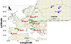 |
Figure 1 Locations of the measurement stations used in the study. Red diamonds denote the ionosonde stations, green stars mark the GNSS stations, whereas the blue and magenta markers on the inset denote the transmitters and receivers of the Doppler Sounding System. |
List of observation sites (ionosondes, CDSS transmitter and receiver antennas, GNSS stations) used in this work.
Automatic scaling of ionograms recorded at the above-listed stations every 5 min has been visually checked for the investigated period with a special focus on the occurrence and intensity of MSTID activity presented in the ionograms at the different stations. For this purpose, the ionograms were carefully manually evaluated (one by one) by the same researcher to minimise the subjectivity of the classification. The MSTID activity was considered if at least two ionograms contained the TIDs signature during the current hour. The intensity of the activity has been divided into four groups (Table 2), based on the frequency range of the ionograms affected by the TIDs signature (fork shape, satellite trace, multiple cusps, etc., see Table S1 in Supplementary material). Moreover, the Sporadic E (Es) activity recorded at the different stations during the investigated period has also been checked and indicated, since the presence of an Es layer can affect the appearance of the TID signature above, especially if it blankets the part of the F layer. The images of the used ionograms from the seven stations are openly available on the GIRO website.
Classification of the Ionograms based on the frequency range affected by the TIDs signature.
2.4 Continuous Doppler sounding system
Multi-frequency (different reflection heights) and multi-point CDSS sounding are performed in the Czech Republic. Figure 1 (zoomed subplot) shows the locations of Doppler transmitters and receivers. Frequencies of 3.59, 4.65, and 7.04 MHz are transmitted by transmitters Tx1, Tx2, and (see Table 1 and Fig. 1). Receiver Rx1 (Table 1) is located at the Institute of Atmospheric Physics, Prague. Digisonde DPS4D (50.00°N, 14.60°E) is close to Tx2 and makes it possible to estimate the reflection heights of the Doppler sounding signals. TIDs induce plasma motion (changes) that cause the Doppler shift of the received signals reflected from the ionosphere. Data processing and analysis run in several steps. First Doppler shift spectrograms are computed. Next, the maximum spectral intensity at each time (usually with a time resolution of 30 or 60 s) is found to obtain time series (single-value functions of time) of Doppler shifts for each sounding path (transmitter-receiver pair). This step is done automatically but visually checked and corrected if needed (e.g. outliers due to electromagnetic interference, visual check was performed for the whole analysed period and the manual correction was necessary approximately once an hour on average during this time). Finally, velocity components and directions of TID propagation, including their uncertainties, can be estimated from the time delays between Doppler shift fluctuations (waves) recorded for different sounding paths and known distances of reflection points. The time delays are found for the times of best cross-correlation between Doppler shift time series for individual sounding paths and from the times obtained by the best beam slowness search. The differences between time delays obtained by different methods serve to estimate the uncertainties of the calculated velocities and azimuths. See the papers by Chum & Podolská (2018) and Chum et al. (2021) for a more detailed description of the applied propagation analysis. A two-dimensional version was used in this study to perform the analysis over as large intervals as possible (Chum et al., 2021).
2.5 Digisonde-to-digisonde oblique sounding
The High-Frequency Travelling Ionospheric Disturbance (HF-TID) method, or Digisonde-to-Digisonde (D2D) oblique sounding technique, also employs high-frequency radio wave remote sensing to study ionospheric irregularities and disturbances. Pairs of identical Digisondes, (sounding paths used in this study: Průhonice–Sopron, Juliusruh–Dourbes, Dourbes–Ebro; the coordinates of the used stations are seen in Table 1) are synchronised, one Digisonde is transmitting and the other one is receiving the signal. This allows accurate measurements of characteristics of travelling ionospheric disturbances in the ionospheric reflection area close to the midpoint of a distinct D2D radio link.
160-minute time series of D2D output products, known as oblique skymaps, are used to detect TIDs. Using the Doppler-Frequency-Angular-Sounding (FAS) technique described in Paznukhov et al. (2012), this method allows for estimating the various TID parameters, including velocity, wavelength, and amplitude and provides insights into the direction of propagation and periodicity of the disturbances.
To achieve reliable characterisation of the detected TIDs, the D2D measurement needs to select a suitable operating frequency which can be used over a long period (one frequency for day and one for night, respectively). Further operational details are discussed in Verhulst et al. (2017).
The combination of the D2D technique and vertical soundings enhances the spatial resolution and accuracy of ionospheric observations compared to single-station measurements. It provides valuable data for mapping ionospheric conditions over large areas and helps in studying the propagation of ionospheric disturbances, like TIDs. The scientific application of this method has been tested in various projects investigating TIDs, including the Pilot Ionosonde Network for Identification of Travelling Ionospheric Disturbances (NetTIDE) in Reinisch et al. (2018) and references therein. The distance between the D2D stations involved and the measurement cadence (2.5 or 5 min) is more suitable for the detection of LSTIDs compared to MSTIDs. The results of the D2D measurements during the investigated period are seen in Section 3 in Supplementary material.
2.6 Total electron content data
Due to the nature of GNSS measurements, we can derive the TEC of the ionosphere along the line of sight between the GNSS receiver and the satellite. This technique leverages dual-frequency phase measurements. The TEC derived from GNSS differs from ionosonde measurements: ionosondes measure the electron density profile from the bottom of the ionosphere to its maximum while TEC measurements integrate the electron density along the entire ray path. Therefore, applying both measurement techniques in parallel will allow us to gain a more accurate and complete picture of TID activity during the periods of interest. To derive the vTEC (vertical TEC), we used the NeQuick calibrated geometry-free linear combination (GFLC) of phase measurements, as detailed in Guerra et al. (2024). To derive the vTEC from the slant observable, the single-layer approximation is applied. The ionosphere is approximated as a 2D layer, fixed at a certain altitude (300 km). Thanks to this widely used approximation, it is possible to apply a mapping function that projects vertically the slant measurements (Mannucci et al., 1998). Here, by exploiting the NeQuick 2 model (Nava et al., 2008) to estimate the bias, it is possible to reduce the effect of the projection of the calibration bias, which is constant for sTEC arcs while it is a function of the elevation angle for vTEC arcs. The mapping and calibration process explained above are follows:
 (1)
(1)
where vTEC is the verticalised, NeQuick2-calibrated vertical TEC, GFLCPhase is the geometry of a free linear combination of phase measurements, BiasNeQuick2 is the calibration constant bias (equal to a climatological value of the sTEC), Re is the Earth’s radius, θ is the elevation angle, and HIPP is the height of the ionospheric layer. The right-hand side of the multiplication in equation 1 is the mapping function, while the left side represents the calibrated observable.
Typically, TID studies merge a large number of observations to remove the effect of GNSS satellite movement, which is complex. However, in this study, we used the BeiDou C05 satellite, a geosynchronous orbit (GEO) satellite visible by GNSS receivers in the European sector. GEO satellites are observed at a fixed longitude, meaning their ionospheric piercing point remains fixed in space under the assumptions stated before. This removes the influences of satellite-ionosphere relative motion, elevation and TEC spatial gradients on the vTEC time series. Once the GEO vTEC time series is obtained, one needs to remove the background variations unrelated to the passage of the MSTID, such as day-to-day variability and diurnal variations. To do this, we applied a detrending technique called Savitsky-Golay filtering (Schafer, 2011), a polynomial detrending performed on a sliding window. For our study, the detrending window was set to 1 h and the polynomial order to three. To better highlight the different frequency components related to the MSTID passage, we performed a time-frequency analysis by leveraging the wavelet synchrosqueezed transform (Daubechies et al., 2011).
Nowadays, data gathered by thousands of GNSS receivers is available worldwide and freely accessible. Because of this, it was possible to find four GNSS receivers closely located to the Průhonice, San Vito, Sopron and Ebro ionosonde sites. Unfortunately, it was not possible to exploit observations gathered by GNSS stations colocated with the Juliusruth and Dourbes ionosondes, as the C05 satellite is not visible at such latitudes. The four GNSS stations are named EBRE, GOPE, GRAZ and MATE (see Table 1 and Fig. 1) and belong to the EUREF permanent GNSS network (EPN; Bruyninx et al., 2019). The data used have a time resolution of 30 s, enough to study MSTIDs, usually characterised by periods of tens of minutes.
3 Observations
3.1 Meteorological situation
3.1.1 Synoptic situation 25–30 August 2023
The advection of warm and humid air into central Europe during the analysed period happened between a cyclone over the North Sea and an anticyclone over eastern Europe. A tropospheric cold front separated the colder polar air mass covering western and, later in the period, all of central Europe from tropical air over Eastern Europe throughout the period. At the surface, the cold front extended in a deep pressure trough related to a cyclone centred over the North Sea (Fig. 2a). Here, due to local changes in surface pressure caused by the rugged orography, it began to wave and its eastward progress was considerably retarded (see Figs. 2b–2f). In the upper troposphere, the cold front was associated with the meridional polar jet stream. The jet stream extended across Europe from the North Sea through central Europe to the Iberian Peninsula along the region of the surface front (Figs. 3a–3f). (With increasing altitude, the axis of the atmospheric front shifted more westward, into the region of cold air close to the surface). The quasi-stationary meridional jet stream fixed the pressure field in a stationary pattern over the entire vertical extent of the troposphere for an unusually long period of several days. On 26–27 August, wind speeds along the jet stream axis exceeded 200 km/h (shown in yellow in the region over Western Europe in Figs. 3c–3f), an unusually high speed for the summer season, when jet stream speeds typically do not exceed 160 km/h (Conway, 1997). Thunderstorms formed in the unstable air mass ahead of the cold front. Tropical air near the ground provides the moisture and energy needed for the strong updrafts that generate radial gravity waves. The unusually persistent meridional jet stream maintained a strong vertical wind shear across the entire troposphere, which caused the storms to be tilted. Tilting is necessary to prevent the updraft in storms from being terminated by the downdraft, so it is a necessary condition for persistent organised storms.
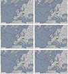 |
Figure 2 Surface pressure maps provided by the Deutscher Wetterdienst available at https://www.wetterzentrale.de/de/reanalysis.php?map=1&model=dwd&var=45, accessed on 19 January 2025, geographical coordinates and a layer with a map of the Czech Republic was added. Surface pressure is represented by solid lines with 10 hPa steps. Atmospheric fronts (red line with semicircles indicating the direction of the warm front, blue line with blue triangles indicating the direction of the cold front, and purple lines with alternating triangles and semicircles indicating the direction of the occluded front) and the locations of the centres of high (H) and low (T) pressure systems are also shown. The orange branch line indicates a squall line. |
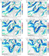 |
Figure 3 The jet stream (colour scale) and wind speed and direction (grey contours with arrows) at the 300 hPa level (~9500 m) over Europe between 25 August 12 UTC and 28 August 00 UTC, 2023. Available at https://www.firenzemeteo.it/en/maps/archive-gfs-weather-forecast-and-analysis-maps.php, accessed on 19 January 2025. |
3.1.2 Strong jet-front system with Mesoscale Convective System event 26–27 August 2023
A period of extreme jet stream and storm intensity was preceded by several hot days defined by a weak anticyclonic pressure field over continental Europe. A 30-year temperature record was measured at half of the ground stations in the Czech Republic. As a result, on the evening of 24 August and during the day on 25 August, there was not enough moisture in the middle and upper troposphere to produce long-lived organised convection (Fig. S2A in Supplementary material). Nevertheless, intense single-cell thunderstorms accompanied by severe winds and large hail occurred over western and central Europe ahead of the cold front.
On 26 August, a cold front moved into central Europe. The strong contrast between the drier and cooler polar air mass over Western Europe and the moist and hot air in the lower troposphere over Central and Eastern Europe is evident in the pseudo-equivalent temperature field (Fig. 4a). The convective environment ahead of the cold front was suitable for the formation of long-lived supercells, based on radiosonde measurements (see Fig. S2B in Supplementary material). There was enough humid, unstable air throughout the troposphere (CAPE values in Central Europe reached up to 1700 kJ/kg), and the strong flow changed direction with height (wind shear values at 0–6 km exceeded 20 m/s). The wind shear in the lower half of the troposphere is also evident in the reanalysis of the surface pressure field and the 500 hPa field (Fig. 4c – Near the surface, the wind was blowing along the isobars (white line) from the west in front of the cold front and the east behind a cold front crossing the centre of the Czech Republic. In the middle troposphere, air from the southwest flowed along the 500 hPa pressure isolines (black lines) over the whole of Europe).
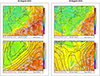 |
Figure 4 Upper Panels: Pseudo-equivalent potential temperature at the 850 hPa pressure level (colour scale, 3 °C spacing and grey isotherms, 1.5 °C spacing) and surface pressure field (white contours, 2 hPa spacing). The theoretical pseudo-equivalent temperature is higher than the “normal” temperature by the specific heat of the water vapour contained in the air mass. It therefore includes information about both the temperature and the humidity of the air mass. Bottom Panels: Distribution of the geopotential height of the 500 hPa level (black lines, 4 decameter spacing), the temperature at the 500 hPa level (grey dashed lines, 5 °C spacing), the surface pressure field (white lines, 2 hPa spacing) and the relative topography between 500 and 1000 hPa (colour scale, 4 decametres) – represents the vertical distance between the 1000 hPa level (surface) and the 500 hPa level (middle troposphere, about 5.5 km) and varies with temperature and humidity – orange/red values indicate tropical air masses and yellow/green indicate polar air masses. a) and c) on 26 August 2023, 18 UTC; b) and d) on 28 August 2023, 18 UTC. Available at https://www.wetterzentrale.de/de/reanalysis.php?map=1&model=dwd&var=45, accessed on 19 January 2025. |
The critical superposition of extreme air mass lability and strong vertical wind shear in the area of Central Europe was enhanced by the lifting caused by the presence of the 500 hPa pressure trough centred over the Czech/Austrian border and filled with relatively cold air (Fig. 4c).
During the midday hours, two supercells formed in front of a cold front over the Transalpine region of Bavaria and merged to form a continuous linear mesoscale convective system (MCS), which reached Austria and the Czech Republic in the evening. The radar image shows this linear system of thunderstorms, which is bowed in the direction of the system’s progress (see Fig. 5). The so-called “bow echo” on a radar image always indicates the presence of severe thunderstorms. According to the European Severe Weather Database (ESWD) records, wind gusts of an intensity that met the definition of a derecho event (wind speed greater than 25 m/s over an area greater than 400 km) were recorded along the linear MCS. In Central Europe, the number of warm-season derechos (from April to September) varies strongly from year to year, but at most, there are only a few cases per year. They move from the south and southwest and are most frequent in central and western parts of Europe (Surowiecki et al., 2024).
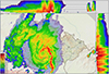 |
Figure 5 The Czech Weather Radar Network (CZRAD) composite of maximum reflectivity (dBZ, see the dBZ scale at bottom left) in pseudo-3D-view shows the structure of the MCS cloud. The image shows the maximum dBz at all heights and its horizontal structure. The side projections show the maximum dBz for a given direction and altitude (from 1 to 14 km, with solid lines at altitudes of 5, 10 and 14 km). This can be used to estimate the location and altitude of maximum radar reflectivity. The white areas correspond to the highest dBZ values (The circle artefacts around the radar location are the effect of the radar scanning and image processing technique.) (Setvák et al., 2010). Data source: Czech Hydrometeorological Institute, processing P. Novák. |
The satellite image shown in Figure 6 illustrates the extensive anvil cloud top above the core of the Mesoscale Convective System (MCS). About an hour before sunset, the active part of MCS covered most of the Czech Republic and a large part of Austria. The coldest parts of the storms (sharp spots of darkest red) are so-called overshooting tops – parts of the storms where the convective updraft penetrates the equilibrium level of the cloud tops and reaches up to 2 or 3 km into the lower stratosphere. According to radiosonde measurements, the tropospheric height over central Europe was about 12 km at 18 UTC on 26 August (Fig. S2B, bottom panel in Supplementary material). Overshooting tops are a very effective source of GW, as shown by the waves visible in the extensive cirrus cloud cover of this MCS. The propagation of concentric GWs generated by the overshooting tops in the horizontal plane is visible over the non-turbulent part of the MCS (western part of the MCS in the satellite image). Close to the active centre of the MCS (the manifested by the overshooting tops), a wide range of interfering waves is present. As a result, the wave structures in the northern and eastern parts of the MCS are disturbed. In the southeastern part of the MCS, a new MCS core is growing, so GWs are not visible in this region. The peaks of the storms associated with the MCS roughly co-locate with the linear structure of the maximum reflectivity (white and dark red colour) in the radar image of Figure 5.
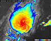 |
Figure 6 Colour-enhanced AVHRR IR band 4, NOAA-19 polar-orbiting satellite, showing a mesoscale convective system (MCS) on 26 August 2023 at 19:12 UTC. Data source: NOAA and CHMI, processing and visualisation by M. Setvák, CHMI. The colour scale indicates the temperature of the upper cloud boundary of storms at a height of about 10–13 km. The coldest tops of storms (in red) reach temperatures as low as −70 °C (Setvák et al., 2008). |
Lightning activity along the cold front on 26 August was also exceptional (Fig. S4B in Supplementary material). According to the Czech Hydrometeorological Institute (CHMI), the 24-hour lightning activity on the territory of the Czech Republic, recorded by the Blitzortung lightning detection network, was the highest in the last 10 years.
It can be assumed that the jet stream itself was a significant source of gravity waves on 26 August. Firstly, because Central Europe was located below the jet stream exit region in front of the low-pressure trough in the upper troposphere (Figs. 3c and 4c). This area is considered to be a region of enhanced gravity wave activity (Plougonven & Zhang, 2014). Second, the extreme values of wind speeds near the tropopause, which reached up to 200 km/h (according to model reanalyses; Fig. 3c) and radiosonde measurements (Fig. S2B in Supplementary material). These are unusually high values for a summer polar jet stream (Conway, 1997).
3.1.3 Thunderstorm activity 28–29 August 2023
Figures 2b–2d and Figures 4a and 4b show a very gradual shift of the cold front. On 26 August, the largest temperature gradient was at the border between Germany and the Czech Republic, and on 28 August the front was only 400 km further east at the border between the Czech Republic and Slovakia. In areas of tropical air masses (the hottest red in the pseudo-equivalent temperature reanalysis in Fig. 4b) in Slovakia, eastern Poland and Hungary, the ESWD reported severe thunderstorms with dangerous downbursts and hail in the afternoon. The existence of a strongly convective environment, supporting the generation of severe thunderstorms and also gravity waves with a vertical component of propagation, is evidenced by the values of convective parameters calculated from radiosonde measurements of vertical profiles of the troposphere. (In Central Europe, the CAPE exceeded 2700 kJ/kg at 12 UTC, and the deep wind shear at 0–6 km was 11 m/s, see Fig. S2C in Supplementary material.) The existence of a strong wind shear in the lower half of the troposphere is confirmed by the reanalysis of the flow at the surface and at 500 hPa (white and black lines in Fig. 4d).
On 29 August, numerous single-cell thunderstorms occurred in the afternoon in the frontal area over eastern Poland, without any severe weather being reported, and also over western Hungary, where a local low in the lower troposphere formed near the ground due to continued warm advection from the south.
On 30 August, a cooler westerly flow (wind flow from the west) prevailed over Europe over land without significant dynamic changes in the troposphere.
3.2 Geomagnetic observations
As for geomagnetic conditions, according to the NOAA SWPC PRF 2504 issued on 28 August 2023 (https://www.ncei.noaa.gov/products), none of the CMEs observed in available coronagraph imagery appeared to be on the Sun-Earth line during the analysed period. No proton events were observed at geosynchronous orbit. The greater-than-2-MeV electron flux at geosynchronous orbit remained at low to moderate levels throughout this period. Geomagnetic field activity ranged from quiet to active conditions. Figure 7 shows geomagnetic and interplanetary conditions during the considered period: a single period of active conditions was observed early morning on 27 August due to a period of sustained Bz south that reached −7 nT. The Kp maximum was 3+, Dst minimum reached the −15 nT value, while the Ap index maximum was 17 during the morning hours of 27 August (Fig. 7). Nevertheless, no increased values of IL, IU, IE can be observed in this period. Only quiet to unsettled conditions were observed for the remainder of the analysed period. On 25 August, the IL and IE indices reached −500 nT and 500 nT, respectively (Fig. 7). A slight activity can be seen in the IU and IE indices with approximately 500 nT on 28 August.
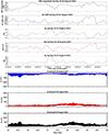 |
Figure 7 The variation of the IMF magnitude and Bz GSM, as well the Kp, Dst, Ap, IL, IU and IE indices for 25–29 August 2023. |
3.3 Ionograms
Examples of ionograms recorded at Průhonice during the investigated period are shown in Figure 8. A review of the ionograms shows that the TID activity was very variable during the studied period. There were ionograms without any TID signatures (e.g. Figs. 8a and 8c), in some cases multi cusp and fork shapes appeared, but the distortion affected only a small frequency range (<1.5 MHz, Figs. 8b, 8d, 8e, and 8f), and sometimes ionograms showing very distorted traces were recorded (Figs. 8g–8l). According to 2-D and 3-D magnetoionic ray tracing models (Cervera & Harris, 2014; Laryunin, 2021), the observed signatures (fork (Y/U) shape, multi cusp and other loops) are usually associated with medium-scale TIDs, while large-scale TIDs (period: >45 min) mainly cause rising and falling values of h’F2 but not distortions seen within a single ionogram. According to the literature (e.g. Cervera & Harris, 2014; Verhulst et al., 2022), variations in the h’F (hmF2) and MUF parameters can show the TID activity. We compared h’F2 and MUF observed during daytime when there were essentially no TID signatures on the ionograms (08–10 UT on 25 August) with the same parameters observed during the time of the very distorted traces observation (08–10 UT on 27 August). While no clear changes can be detected in the parameters on the 25th (Fig. S10A in Supplementary material), periodic changes, especially in the h’F2 (periods: ~15–20 min) can be seen on 27 August (Fig. S10B). This indicates that TIDs of various scales are present simultaneously. Additional examples of ionograms, including from other observatories, are shown in Section 2 of the Supplementary material (Figs. S8A, S8B, S9B, and S11).
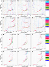 |
Figure 8 Examples of ionograms recorded at Průhonice station during daytime (08–11 UT) on 25 August (a–c), on 26 August (d–f) and on 27 August (g–i). F traces without TID signatures (white in Table 3) are shown in Figures 8a and 8c, while weak TID signatures which affect <0.5 and 0.5 < f < 1.5 MHz frequency range are seen on plots b, d, e and f respectively (pale orange colours in Table 3). Very distorted ionograms (essentially the whole observed F trace is affected) are seen on plots g–i. All times are given in UT. |
Table 3 shows the occurrence and intensity of MSTID activity present in the hourly ionograms at the different stations. We consider MSTIDs to be present if at least two ionograms in the hour show TID signatures. The different colours indicate the intensity of the TID activity as it appeared on the ionograms. The palest orange shows the periods when the affected frequency range on the ionograms by the TIDs signature (fork shape, satellite trace, multiple cusps, etc.) was less than 0.5 MHz. In the cases of the darkest orange periods, most of the F trace was significantly distorted (see the legend in the left upper corner of Table 3, and also Table 2). The presence of a sporadic E layer can affect the detection of TID signatures on the F trace, especially in the case of the blanketing Es, which partially or completely obscure the overlying F layer. Therefore, the Es activity is also indicated in the Table with the label “Es”.
Summary of the TID activity observed in the traces of the ionograms at European stations during the front passage between 25 and 29 August 2023 (the dates can be seen in the first column). The columns indicate the hours in UT. The investigated stations are DB049, EB040, EA036 from North to South in the Western Europe longitudinal sector, and JR055, PQ052, SO148, and VT139 from North to South in the Central Europe longitudinal Sector (see Fig. 1). The colours indicate the intensity of the TID activity as seen on the ionograms (if at least two ionograms during that hour were affected). Light orange is used when the affected frequency range is less than 0.5 MHz, while the darkest orange denotes the case if most of the F trace was distorted. The presence of a Sporadic E layer is indicated with the label “Es”.
Very strong MSTID activity with extremely distorted F traces on the ionograms was observed at the higher mid-latitude stations (Dourbes, Juliusruh, Průhonice, and Sopron), especially on 27 and 28 August 2023. The occurrence rate and the intensity of the MSTIDs at the different stations were much higher than the MSTID occurrences recorded in a quiet period, the first part of September 2014 (a similar hourly rate analysis was done manually for this period, when the solar activity was high as in 2023). The intensity of the MSTID activity seen in the ionograms can be recognized despite the presence of the Es layer in some cases. Therefore, based on the analysis of ionograms, we can conclude that the presence of the extremely strong tropospheric event had a great impact on the occurrence of MSTID activity on 27 and 28 August. It is worth noting that more intense MSTID activity was recorded at the higher midlatitude stations in both the Western- and Central-European longitudinal sectors. However, a clear propagation pattern, e.g. the disturbance moving from North to South or from West to East, can not be identified based on the results shown in Table 3. The reason for the ionosonde network not being able to unambiguously determine the propagation azimuth of the TIDs in the present case may be the sparsity of the ionosondes and the temporal resolution of ionogram soundings. Furthermore, multiple processes were present in parallel besides the effect of the orography of the Alps (increased jet stream, severe convection at more locations), which were capable of generating atmospheric gravity waves. Thus, a clear propagation pattern cannot be as easily determined as in the case of a singular source (especially if one knows the location and the exact time of the source, e.g. Hunga Tonga or the Turkey Earthquake on 6 February 2023, Verhulst et al., 2022; Haralambous et al., 2023).
3.4 Continuous Doppler sounding system observations
CDSS measurements at 7.04 MHz reflected from 200 to 320 km height (Fig. 9, right) also indicated very high MSTID activity during the daytime for soundings on 26, 27 and 28 August 2023. Sounding at a lower frequency, 4.65 MHz (Fig. 9, left) showed just small Doppler shift variations during the daytime due to the prevailing reflection from the E or F1 layer. Spectral analysis of sounding at 7.04 MHz (Fig. 10, right side) showed that the dominant period of the daytime TIDs was around 20 min. Large waves were observed mainly on 26 August from about 11–15 UT and on 27 August from approximately 6–13 UT. These intervals are also marked in Figures 9f and 9g by rectangles (magenta). Propagation analysis, described in Section 2.4 and displayed on the right side of Figure 10 for 7.04 MHz, shows prevailing eastward or east-northward propagation. On the other hand, the most active period was detected on the evening of August 28 with north-westward propagation (approximately from 17 to 20 UT). Moreover, northward and north-westward propagated TIDs were observed at 7.04 MHz in the afternoon-evening hours on 26 August, thus at the time when the MCS occurred in the territory of Austria and Czechia. Only azimuths for large fluctuations (absolute value of Doppler shift larger than 0.1 Hz) and with estimated uncertainties in azimuth smaller than 10° are shown in Figure 10. The CDSS records for 4.65 MHz (reflections from 140 to 220 km range during daytime and 260 to 360 km during night, please see Figs. S12A and S12A in Supplementary material) also indicate MSTID activity during the investigated days (Fig. 9, left side), mainly. An active period was detected in the early morning (01–04 UT) on 25 August, with a peak period of ~30 min. and east-northward propagation (Fig. 10, left side). Furthermore, very active periods are seen in the evening/night of 27–28 August (mainly east-northward propagation), and another peak in the evening hours on 28 August (with north-west propagation direction). It is important to note that at the frequency of 4.65 MHz, the signal is reflected from the F2 region during the evening-night hours and from the E or F1 layer during the day (see Figs. S12A and S12A). The Doppler shifts of waves reflecting from these lower layers are very small. On the other hand, the 7.04 MHz signals reflect from the F layer during the day and experience relatively large Doppler shifts. However, the critical frequency foF2 is usually lower than 7 MHz at night, and the signals transmitted at this frequency escape to outer space (do not reflect). Spectral and propagation analysis presented in Figure 10 was done for the intervals with available signals (Figs. 9, 10a, 10d).
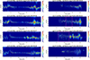 |
Figure 9 Doppler shift spectrograms recorded at f = 4.65 MHz (left side, a–d) and at f = 7.04 MHz (right side, e–h) for the Tx1–Rx1 sounding path from 25 to 28 August 2023. |
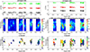 |
Figure 10 The top panel shows Doppler shift (signals from individual transmitters are artificially offset by about 4 Hz) for the analysed period at 4.65 MHz (left side, a–c) and at 7.04 MHz (right side, d–f), while the panels in the middle and at the bottom give information on RMS values of Doppler shift in different frequency (period) bands and azimuths of the wave propagation, respectively. |
3.5 Total electron content observations
The GNSS receiver colocated with the Ebro ionosondes did not show clear MSTID signatures in the dTEC time series during the investigated period. The one in San Vito showed signatures only during the daytime on 27 August; they are thus only shown in the Supplementary material (Figs. S14 and S15).
Figure 11 and 12 show the GEO vTEC, detrended vTEC (dTEC) along with moving standard deviation calculated on a 45-minute sliding window, and the wavelet analysis of vTEC for the measurements derived from the GNSS receivers colocated with the Průhonice and Sopron ionosondes respectively. Looking at the whole time series, it is possible to notice how the 27th of August is characterised by dTEC variations stronger than the ones for the previous and following days. Looking at the dTEC panel, the morning hours (4:00–13:00 UT, highlighted in red) of 27 August show the strongest TID signatures, with amplitudes as high as 0.9 TECU for both Sopron and Průhonice receivers. Similarly, the moving standard deviation peaks at 0.46 and 0.38 TECu for Průhonice and Sopron, respectively. By comparing the moving standard deviation with the previous and following days, the maximum value relating to noon hours almost doubles with respect to background values (always smaller or around 0.25 TECu). Weaker TID activity is also visible in the evening-night hours of the 27–28 (highlighted in blue in the dTEC panel), with lower amplitudes than daytime TIDs. This lower amplitude is explained by the fact that TIDs are driven by collisions between the underlying neutral wave and ionospheric particles. Thus, a lower background ionisation will cause a smaller amplitude due to the lower amount of plasma displaced. Nevertheless, even if the amplitude is smaller (0.3 TECu), comparing it with nighttime values for the other days considered shows how the amplitude is twice as high for the nighttime between the 27 and 28 of August. The same pattern is shown by the moving standard deviations, with peaks reaching 0.23 and 0.17 TECu for Průhonice and Sopron, respectively. Again, these peak values visible in the blue-shaded area are unmatched during the previous/following days. The wavelet analysis shown in the bottom panels is really helpful for investigating the specific periods activated by the passage of the TIDs, as the dTEC does not provide such detailed temporal information. For the Průhonice GNSS receiver, the wavelet spectrogram shows increased activity defined by periods around 40 and 25 min during the daytime (red patch in the dTEC panel). During nighttime (blue patch), the main period is instead around 30–35 min. By comparing the wavelet spectrogram with the RMS values of Doppler shift in different frequencies shown in Figures 10b and 10e, it is possible to note how the periods visible in TEC are in accordance with CDSS. Specifically, CDSS shows an intensification of periodicities around 30 min in the 27–28 August nighttime (4.65 MHz, Fig. 10b) and around 15–25 minutes in the pre-noon hours (7.04 MHz, Fig. 10e). When comparing GNSS TEC and CDSS, one has to remember that while TEC is an integrated quantity showing the sum of all density disturbances along the receiver-satellite line of sight, CDSS instead measures the plasma drift fluctuations at a specific ionospheric density/height. Thus, a direct comparison between the two instruments is indeed not straightforward, and could be a possible topic for further investigation. Despite that, the two measurement techniques show a reasonable degree of accordance in the wave periods for the pre-noon and pre-midnight hours of the 27th of August. Sopron GNSS TEC shows a similar behaviour, with the daytime showing fluctuations defined by periods around 40 and 25 min and the nighttime between 30 and 40 min. As MSTIDs are a common phenomenon, observing coherence in both the time and amplitude of the increased TID activity between two different sites (Průhonice and Sopron) confirms that something causes this deviation from the typical day-to-day variability. Moreover, as the front system was mainly localised over Central Europe, no increased MSTID activity for Ebro GNSS stations located in Spain confirms that such behaviour is likely connected to the tropospheric event.
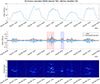 |
Figure 11 Top panel shows the GNSS single station TEC, middle panel shows the dTEC along with the moving standard deviation calculated on a 45-minute sliding window. Bottom panel shows the wavelet spectra at the stations co-located with Průhonice from 25 to 29 August 2023. |
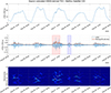 |
Figure 12 Top panel shows the GNSS single station TEC, middle panel shows the dTEC along with the moving standard deviation calculated on a 45-minute sliding window. Bottom panel shows the wavelet spectra at the stations co-located with Sopron (lower part) from 25 to 29 August 2023. |
4 Discussion
In the period of 25–29 August 2023, a strong jet-front system passed through continental Europe (Fig. 2). The tropospheric cold front separated the colder polar air mass covering Western and Central Europe from tropical air over Eastern Europe throughout the period (Fig. 4). The cold front extended in a deep pressure trough related to a cyclone centred over the North Sea at the surface level. While in the upper troposphere, the cold front was associated with an extensively long (from the North Sea to the Iberian Peninsula) meridional polar jet stream, with exceptionally strong wind speeds for this season (200 km/h on 26–27 August, see Fig. 3). The convective environment ahead of the cold front was suitable for the formation of long-lived supercells, therefore, intense thunderstorms occurred with very high numbers of lightning (see Fig. S4 in Supplementary material). The intense convection and the unusually persistent meridional jet stream caused a strong vertical wind shear across the entire troposphere, which was favourable for generating atmospheric gravity waves. A continuous linear mesoscale convective system (MCS) formed in the Austrian-Czech Republic region in the afternoon-evening hours on 26 August. The overshooting tops of the MCS – the coldest parts of the storms where the convective updraft penetrates into the stratosphere – were also a very effective source of GWs (see Fig. 6). It is important to note that the geomagnetic conditions can be considered quiet during the passage of the frontal system (Sect. 3.2, Fig. 7).
According to the literature (e.g. Fritts & Nastrom, 1992, Koucká Knížová et al., 2021, 2024), mid-latitude cyclones can trigger AGWs that could propagate upward and reach the ionospheric heights. The main sources of gravity waves in the troposphere besides orography are convection, and jet/front systems, the latter ones dominate over the midlatitudes (Plougonven & Zhang, 2014). Numerous studies using different observational techniques have highlighted a clear enhancement of gravity wave activity in the vicinity of jets and fronts (e.g., Fritts & Nastrom, 1992; Plougonven et al., 2003). Moreover, several case studies reported the occurrence of strong gravity wave events in the vicinity of a jet/front system (Uccelini & Koch, 1987; Guest et al., 2000). Wave-like perturbations of the ionospheric plasma were observed quasi-immediately after the passage of cold fronts over the observation site in Central Europe (Šauli & Boška, 2001; Sindelarova et al., 2009; Koucká Knížová et al., 2020). The wave-like fluctuations were recorded as changes in ionospheric departures from horizontal stratification, significant plasma flow shears and an increase in the speed of horizontal plasma drifts, increased spread-F activity related to AGWs, and detection of gravity waves by the Continuous Doppler Sounding System (Koucká Knížová et al., 2021, 2023, 2024). When AGWs enter the ionised and magnetically determined thermosphere/ionosphere system, they are also observed as TIDs. TIDs with a wavelength of 50–500 km, periods of 12–60 min, and a propagation speed of 100–300 m/s are classified as MSTIDs (Hunsucker, 1982; Kil & Paxton, 2017).
In the present study TID activity during the passage of a strong jet-front system was investigated by different observational techniques, namely by an analysis of ionograms recorded at seven European ionosonde stations; by Continuous Doppler Sounding System in the Czech Republic; by D2D (Digisonde to Digisonde) data recorded at the Průhonice-Sopron, and Juliusruh-Dourbes path; furthermore by TEC detected at GNSS stations co-located with the ionosondes. The most intense MSTID activity was observed on the ionograms (Table 3) and by single station dTEC measurements (Fig. 12), and also detected by the Continuous Doppler Sounding System at 7.04 MHz during the daytime (~06–13 UT) on 27 August. According to the CDSS records at 7.04 MHz, the dominant period of the daytime TIDs was around 20 min while the direction of propagation was mainly eastward and north-eastward on 27 August (Fig. 10), which means that the source could be westward from the Czech Republic. The wavelet spectrogram of the dTEC recorded at the GNSS station co-located with Průhonice also shows a 20-minute dominant period (Fig. 11). Furthermore, increased activity defined by periods around 20–40 min was identified at both investigated GNSS stations (co-located with Průhonice and Sopron) during the daytime (Figs. 11 and 12). The presence of TID with 30–50 min periods before noon was also supported by the D2D measurements at the Průhonice – Sopron path, too (Fig. S13A in Supplementary material). This period (around noon on 27 August) agrees well with the time when the jetstream reached its highest values (it exceeded 200 km/h, which is an unusually high speed for this season) at a large territory over continental Europe (see Fig. 3e). It is important to note that the geomagnetic conditions were unsettled (Kp = 3+, Dst = −17 nT) in the early morning hours on 27 August. However, the IL, IU and IE indices, thus the proxies for the auroral electrojet activity, did not increase. Furthermore, the CDSS observations show that the propagation of the TIDs was mainly eastward and northeastward, which is against the assumption that the source could be in the auroral region; it supports that it could be the strong jet stream above Western Europe. Previous results (Hunsucker, 1982) also showed that the daytime MSTID activity observed in dTEC can be driven by the jet stream during autumn and winter. Based on measurements from GNSS receivers, ionospheric soundings and wind speed data at a tropospheric level Wautelet & Warnant (2015) concluded that tropospheric jetstream can be the most probable source of daytime MSTIDs. Furthermore, Shpynev et al. (2019) reported medium-scale wave-like disturbances in the winter ionosphere caused by the atmospheric waves generated by high-speed jet streams. Spectral analysis of TEC variations showed 10–16 min ionospheric variations over Kaliningrad (higher midlatitude) on the day of a meteorological storm (Borchevkina et al., 2020), the observed periodicities are comparable with our results.
Besides the above-detailed activities, MSTIDs were also observed in the early morning on 25 August and the evening-night periods on 26 and 28 August. An active period was detected in the early morning (01–04 UT) on 25 August, with a peak period of ~30 min and east-northward propagation by the CDSS system at 4.65 MHz (Fig. 10, left side). TIDs with a period of 30–70 min were also observed by the D2D measurement technique in the Průhonice – Sopron path in the same time interval (Fig. S13A in Supplementary material). According to the local meteorological observations at Sopron and the lightning maps (see Figs. S4A, S5, S6 and S7 in Supplementary material) a local thunderstorm occurred over North-West Hungary around 01–02 UT. A large variation in atmospheric temperature and pressure, furthermore, a high intensity of precipitation was recorded. The high number of lightning within a small area suggest locally a strong convection. Intense MSTID activity with periods 15–30 min and 20–50 min was observed at 7.04 and 4.65 MHz, respectively, during daytime and the evening hours on 26 August (Fig. 10). The propagation direction of the disturbances cannot be clearly determined based on the observations. D2D measurement in the Průhonice – Sopron path also observed MSTID activity with periods up to 60 min during the daytime and with ~50 min periods in the evening hours on 26 August (Fig. S13A in Supplementary material). Interestingly, this activity is not that evident on the ionograms recorded at Průhonice and Sopron (Table 3) and at the TEC observations at the co-located GNSS stations (Figs. 11 and 12). Although, the presence of TID signatures on the ionograms were more common at Průhonice in the afternoon hours than at the same time in the days before and after (Table 3). The daytime and evening hours of 26 August agree with the periods when the continuous linear mesoscale convective system (MCS) formed in the Austrian-Czech Republic region. According to the satellite images (Fig. 6), the overshooting tops of the MCS were very effective sources of AGWs. The CDS system detected northward and northwestward propagated TIDs at 7.04 MHz during this period. Considering the territory of the transmitter and receiver antenna system of CDS, the determined propagation direction confirms that the most probable source of the AGWs could be the MCS situated south-south-eastward from it. Moreover, a very active period was detected at 7.04 MHz and also at 4.65 MHz, with a period of 15–30 min and northwestward propagation direction over the Czech Republic by the CDS system in the afternoon/evening hours on 28 August (Fig. 10). Severe thunderstorms (see Fig. S4D in Supplementary material) with dangerous downbursts and hail occurred in the Eastern Poland-Slovakia-Hungary line in the afternoon on 28 August. The presence of a strongly convective environment facilitated the generation of gravity waves with a vertical propagation component, as confirmed by convective parameters calculated from radiosonde measurements (the CAPE exceeded 2700 kJ/kg at 12 UTC, Fig. S2C in Supplementary material). The propagation direction of the observed TIDs (northwestward) also support our presumption that the source of the activity could be the severe thunderstorms over Slovakia and Hungary. It is worth noting that MSTIDs occurring during nighttime can be caused by the electrodynamical processes, e.g. Perkins instability associated with E- and F-region coupling processes (e.g. Cosgrove et al., 2004; Otsuka et al., 2013). However, when we observed the most active nighttime MSTIDs on ionograms (27 August) or by CDSS (28 August), there was no sporadic E activity detected on the ionograms at Průhonice. Thus the ionosonde record does not confirm that those nighttime TIDs can be linked to the coupling between the Es and F layers and Perkins instability.
Fritts & Nastrom (1992) suggested that convective activity in the troposphere can be an important source of gravity waves. Vadas & Nicolls (2012) showed that GWs originating in the tropospheric convection can reach the height of the thermosphere and cause changes in the profiles of wind and temperature there. Yue et al. (2019) reported thunderstorm activity related to concentric acoustic-gravity wave-type disturbances based on satellite observations. The ionospheric response to thunderstorm activity over Europe was also studied through statistical analysis (Davis & Johnson, 2005; Barta et al., 2013) and case studies (Barta et al., 2017; Borchevkina et al., 2020). Concentric wave features and TIDs generated by convective tropospheric sources over the United States were reported by Azeem & Barlage (2018). Hurricane-generated concentric GWs were observed in both the stratosphere and mesosphere and in the ionosphere according to spaceborne satellites and ground-based GPS data (Xu et al., 2019). MSTID activity during two tropical cyclones over the Hong Kong region was verified by Lou et al. (2019) using multi‐instrumental observations (ground‐based GPS networks, ionosonde stations, and Swarm satellites). Our multi-instrumental observations confirm already published findings that tropospheric systems with deep convection can be significant sources of atmospheric gravity waves which reach the ionosphere, leading to MSTIDs.
5 Summary and conclusions
A strong jet-front system dominated the tropospheric weather of continental Europe between 25 and 29 August 2023. The polar air mass moved from the West to Central Europe during this period, displacing tropical air over South-East Europe. The cold front was associated with a long meridional polar jet stream in the upper troposphere, which was accompanied by extremely strong wind speed for this season. Severe thunderstorms occurred during these periods since the convective environment ahead of the cold front was favourable for the generation of long-lived supercells. The above-detailed conditions – the strong vertical wind shear related to the strong convection and to the persistent meridional jet stream – were suitable for the generation of atmospheric gravity waves. While there were calm geomagnetic conditions during those days. Therefore, the combination of such conditions provided an excellent opportunity to study the impact of the jet-front system with severe convection on the ionosphere, especially focusing on the wave-like disturbances – TIDs. In the present study, TID activity during the passage of the jet-front system was investigated by different observational techniques, namely by vertical soundings (ionograms) at seven European Digisonde stations; by Continuous Doppler Sounding System (CDSS) in the Czech Republic; by Digisonde-to-Digisonde (D2D) oblique sounding data recorded at the Průhonice-Sopron, and Juliusruh-Dourbes paths; furthermore by TEC obtained from GNSS stations co-located with the ionosondes. The results of this multi-instrumental investigation can be summarised as follows:
According to the ionogram analysis, to the dTEC records at single stations, and to the CDSS System at 7.04 MHz, the most intense MSTID activity was during daytime (~ 06–13 UT) on 27 August. The dominant period of daytime TIDs was around 20 min, while the direction of propagation was mainly eastward and northeastward. This period (around noon on 27 August) agrees well with the time when the jetstream reached its highest values (~ 200 km/h) over a large territory of continental Europe.
Strong activity of MSTIDs was also observed in the early morning on 25 August and the evening on 26 and 28 August by the CDSS and by the D2D measurements along the Průhonice – Sopron path. The dominant periods varied between 15 and 70 min based on the observations. It was possible in some cases to determine the propagation direction of the disturbance due to the CDSS observational technique. Careful comparison of the time and the direction of TID movement with the meteorological data (satellite image, radar and lightning maps, local meteorological data) shows that the probable source of the MSTIDs was local thunderstorms on 25 and 28 August and the MCS event in Austria/Czech Republic on 26 August.
In conclusion, our multi-instrumental observations confirm already published findings that jet-front systems accompanied by intense convection can be significant sources of atmospheric gravity waves which reach the ionosphere, leading to MSTIDs. Nevertheless, it is important to note that the exact determination of the source of TIDs during such a complex event, as the presented one, is difficult. The most important sources and triggering mechanisms may depend on the season and time of day. It will therefore be important to study more such intense tropospheric events in detail in future. For analyses of this kind, atmospheric/ionospheric data obtained from different sources (multi-instrumental measurements) are very important as they provide the opportunity to capture more accurately the processes under study.
Acknowledgments
The authors wish to acknowledge M. Setvák and P. Novák from the Czech Hydrometeorological Institute and P. Zacharov from the Institute of Atmospheric Physics CAS for providing data and consultations. The authors would like to thank the blitzortung.org project, the Czech Hydrometeorological Institute and Lukáš Ronge, Amateur Stormchasing Society, for access to radar and lightning data. The editor thanks two anonymous reviewers for their assistance in evaluating this paper.
Funding
The authors thank the HORIZON-CL4-2022-Space-01-62 project (Grant Agreement 101081835) “Travelling Ionospheric Disturbances Forecasting System (T-FORS).” The contribution of VB was also supported by the Bolyai Fellowship (GD, No. BO/00461/21). The work of KP, PKK, JC and JU was supported by the Johannes Amos Comenius Programme (P JAC), project No. CZ.02.01.01/00/22_008/0004605, Natural and anthropogenic georisks. Research program Strategie AV21 Dynamicka planeta (Dynamical planet) of the Academy of Sciences of the Czech Republic. The work of PKK, JC and JU was also partly supported by the ESA project QUID-REGIS ESA Contract No. 4000143632/24/I-EB.
Data availability statement
The surface pressure field with synoptic analysis provided by the German Forecast Service (DWD) https://www.wetterzentrale.de/; upper charts provided by http://wetter3.de and https://www.firenzemeteo.it/. The measurement of the vertical profile of the atmosphere is available at https://weather.uwyo.edu/upperair/sounding.html, and the freeware application thundeR for calculation and visualisation of convective parameters provided by http://rawinsonde.com/thunder_app/. Interplanetary magnetic field (IMF) Magnitude (B) and the z component (Bz), the Dst, Kp and Ap indices, the source: https://omniweb.gsfc.nasa.gov/form/dx1.html and for the IE, IU and IL indices, the source: https://space.fmi.fi/image/www/il_index_panel.php. The images of the used ionograms from the seven stations are openly available at the GIRO website: https://giro.uml.edu/ionoweb/. The data of the Continous Doppler Sounding System can be obtained as spectrograms at http://datacenter.ufa.cas.cz/ under the link “Spectrogram archive”. All hourly and daily GNSS data from the EPN stations are made available in the RINEX format at the EPN Regional Data Centres: https://www.epncb.oma.be/_networkdata/data_access/dailyandhourly/datacentres.php
Supplementary materials
Multi-instrument analysis of MSTIDs generated by an intensive jet-front system with severe convection in Europe in August 2023. Access Supplementary Material
References
- Andrews DG, McIntyre MG. 1976. Planetary waves in horizontal and vertical shear: the generalized Eliassen-Palm relation and the mean zonal acceleration. J Atmos Sci 33: 2031–2048, https://doi.org/10.1175/1520-0469(1976)033≤2031:PWIHAV≥2.0.CO;2. [Google Scholar]
- Alfonsi L, Cesaroni C, Hernandez-Pajares M, Astafyeva E, Bufféral S, et al. 2024. Ionospheric response to the 2020 Samos earthquake and tsunami. Earth Planets Space 76: 13. https://doi.org/10.1186/s40623-023-01940-2. [Google Scholar]
- Astafyeva E. 2019. Ionospheric detection of natural hazards. Rev Geophys 57: 1265–1288. https://doi.org/10.1029/2019RG000668. [CrossRef] [Google Scholar]
- Azeem I, Barlage M. 2018. Atmosphere-ionosphere coupling from convectively generated gravity waves. Adv Space Res 61: 1931–1941. https://doi.org/10.1016/j.asr.2017.09.029. [Google Scholar]
- Barta V, Scotto C, Pietrella M, Sgrigna V, Conti L, Sátori G. 2013. A statistical analysis on the relationship between thunderstorms and the sporadic E Layer over Rome. Astron Nachr 334(9): 968–971. https://doi.org/10.1002/asna.201211972. [Google Scholar]
- Barta V, Haldoupis C, Sátori G, Buresova D, Chum J, et al. 2017. Searching for effects caused by thunderstorms in midlatitude sporadic E layers. J Atm Solar-Terr Phys 161: 150–159. https://doi.org/10.1016/j.jastp.2017.06.006. [Google Scholar]
- Becker E, Goncharenko L, Harvey VL, Vadas SL. 2022. Multi-step vertical coupling during the January 2017 sudden stratospheric warming. J Geophys Res: Space Physics 127: e2022JA030866. https://doi.org/10.1029/2022JA030866. [Google Scholar]
- Borchevkina O, Karpov I, Karpov M. 2020. Meteorological storm influence on the ionosphere parameters. Atmosphere 11: 1017. https://doi.org/10.3390/atmos11091017. [Google Scholar]
- Bruyninx C, Legrand J, Fabian A, Pottiaux E. 2019. GNSS metadata and data validation in the EUREF Permanent Network. GPS Solut 23: 106. https://doi.org/10.1007/s10291-019-0880-9. [Google Scholar]
- Cervera MA, Harris TJ. 2014. Modeling ionospheric disturbance features in quasi-vertically incident ionograms using 3-D magnetoionic ray tracing and atmospheric gravity waves. J. Geophys. Res. Space Physics 119: 431–440. https://doi.org/10.1002/2013JA019247. [Google Scholar]
- Conway ED. 1997. An introduction to satellite image interpretation, Johns Hopkins University Press, Baltimore, USA. ISBN 9780801855771. https://doi.org/10.56021/9780801855764. [Google Scholar]
- Cosgrove RB, Tsunoda RT, Fukao S, Yamamoto M. 2004. Coupling of the Perkins instability and the sporadic E layer instability derived from physical arguments. J Geophys Res 109(A6): A06301. https://doi.org/10.1029/2003JA010295. [Google Scholar]
- Chum J, Podolská K. 2018. 3D analysis of GW propagation in the ionosphere. Geophys Res Lett 45(21): 11562–11571. https://doi.org/10.1029/2018GL079695. [Google Scholar]
- Chum J, Podolská K, Rusz J, Baše J, Tedoradze N. 2021. Statistical investigation of gravity wave characteristics in the ionosphere. Earth Planets Space 73: 60. https://doi.org/10.1186/s40623-021-01379-3. [Google Scholar]
- Daubechies I, Lu J, Wu H-T. 2011. Synchrosqueezed wavelet transforms: an empirical mode decomposition-like tool. Appl Comput Harmonic Anal 30(2): 243–261. https://doi.org/10.1016/j.acha.2010.08.002. [Google Scholar]
- Davis CJ, Johnson CG. 2005. Lightning-induced intensification of the ionospheric sporadic E layer. Nature 435: 799–801. https://doi.org/10.1038/nature03638. [Google Scholar]
- Eckermann SD, Preusse P. 1999. Global measurements of stratospheric mountain waves from space. Science 286: 1534–1537. https://doi.org/10.1126/science.286.5444.1534. [Google Scholar]
- Ejiri MK, Taylor MJ, Nakamura T, Franke SJ. 2009. Critical level interaction of a gravity wave with background winds driven by a large-scale wave perturbation. J Geophys Res 114: D18117. https://doi.org/10.1029/2008JD011381. [Google Scholar]
- Figueiredo CAOB, Takahashi CAOB, Wrasse CM, Otsuka Y, Shiokawa K, Barros D. 2018. Medium‐scale traveling ionospheric disturbances observed by detrended total electron content maps over Brazil. J Geophys Res Space Phys 123(3): 2215–2227. https://doi.org/10.1002/2017JA025021. [Google Scholar]
- Frissell NA, Baker JBH, Ruohoniemi JM, Greenwald RA, Gerrard AJ, Miller ES, West ML. 2016. Sources and characteristics of medium-scale traveling ionospheric disturbances observed by high-frequency radars in the North American sector. J Geophys Res Space Phys 121(4): 3722–3739. https://doi.org/10.1002/2015JA022168. [CrossRef] [Google Scholar]
- Fritts DC. 1989. A review of gravity wave saturation processes, effects, and variability in the middle atmosphere. Pure Appl Geophys 130(2–3): 343–371. https://doi.org/10.1007/bf00874464. [Google Scholar]
- Fritts DC. 1984. Gravity wave saturation in the middle atmosphere: A review of theory and observations. Rev Geophys 22: 275–308. https://doi.org/10.1029/RG022i003p00275. [Google Scholar]
- Fritts DC, Alexander MJ. 2003. Gravity wave dynamics and effects in the middle atmosphere. Rev Geophys 41: 1003. https://doi.org/10.1029/2001RG000106. [CrossRef] [Google Scholar]
- Fritts DC, Nastrom GD. 1992. Sources of mesoscale variability of gravity waves. Part II: Frontal, convective, and jet stream excitation. J Atmos Sci 49(2): 111–127. https://doi.org/10.1175/1520-0469(1992)049≤0111:SOMVOG≥2.0.CO;2. [Google Scholar]
- Fritts DC, Rastogi PK. 1985. Convective and dynamical instabilities due to gravity wave motions in the lower and middle atmosphere: theory and observations. Radio Sci 20(6): 1247–1277. https://doi.org/10.1029/RS020i006p01247. [Google Scholar]
- Fuller-Rowell TJ. 1995. The dynamics of the lower thermosphere. In: The upper mesosphere and lower thermosphere: a review of experiment and theory, vol. 87, Johnson RM, Killeen TL (Eds), Washington, DC, American Geophysical Union, pp. 23–36. https://doi.org/10.1029/GM087p0023. [Google Scholar]
- Garcia RR, Solomon S. 1985. The effect of breaking gravity waves on the dynamics and chemical composition of the mesosphere and lower thermosphere. J Geophys Res 90(D2): 3850–3868. https://doi.org/10.1029/JD090iD02p03850. [Google Scholar]
- Guerra M, Cesaroni C, Ravanelli M, Spogli L. 2024. Travelling ionospheric disturbances detection: a statistical study of detrending techniques, induced period error and near real-time observables. J Space Weather Space Clim 14: 17. https://doi.org/10.1051/swsc/2024017. [CrossRef] [EDP Sciences] [Google Scholar]
- Guest FM, Reeder MJ, Marks CJ, Karoly DJ. 2000. Inertia-gravity waves observed in the lower stratosphere over Macquarie Island. J Atmos Sci 57: 737–752. https://doi.org/10.1175/1520-0469(2000)057≤0737:IGWOIT≥2.0.CO;2. [Google Scholar]
- Haralambous H, Guerra M, Chum J, Verhulst TG, Barta V, et al. 2023. Multi‐instrument observations of various ionospheric disturbances caused by the 6 February 2023 Turkey earthquake. J Geophys Res Space Phys 128(12): e2023JA031691. https://doi.org/10.1029/2023JA031691. [CrossRef] [Google Scholar]
- Hertzog A, Boccara G, Vincent RA, Vial F, Cocquerez P. 2008. Estimation of gravity wave momentum flux and phase speeds from quasi-lagrangian stratospheric balloon flights. Part II: results from the Vorcore Campaign in Antarctica. J Atmos Sci 65: 3056–3070. https://doi.org/10.1175/2008JAS2710.1. [Google Scholar]
- Hines CO. 1965. Dynamical heating of the upper atmosphere. J Geophys Res 70(1): 177–183. https://doi.org/10.1029/JZ070i001p00177. [Google Scholar]
- Hines CO, Reddy CA. 1967. On the propagation of atmospheric gravity waves through regions of wind shear. J Geophys Res 72: 1015–1034. https://doi.org/10.1029/JZ072i003p01015. [Google Scholar]
- Hocke K, Schlegel K. 1996. A review of atmospheric gravity waves and traveling ionospheric disturbances: 1982–1995. Ann Geophys 14: 917–940. https://doi.org/10.1007/s00585-996-0917-6. [Google Scholar]
- Hoffmann L, Xue X, Alexander MJ. 2013. A global view of stratospheric gravity wave hotspots located with Atmospheric Infrared Sounder observations. J Geophys Res: Atmos 118(2): 416–434. https://doi.org/10.1029/2012JD018658. [Google Scholar]
- Holton JR. 1982. The role of gravity wave-induced drag and diffusion in the momentum budget of the mesosphere. J Atmos Sci 39: 791–799. https://doi.org/10.1175/1520-0469(1982)039≤0791:TROGWI≥2.0.CO;2. [Google Scholar]
- Holton JR. 1983. The dynamics of large atmospheric motions. Rev Geophys Space Phys 21(5): 1021–1027. https://doi.org/10.1029/RG021i005p01021. [Google Scholar]
- Holton JR, Haynes PH, McIntyre ME, Douglass AR, Rood RB, Pfister L. 1995. Stratosphere-troposphere exchange. Rev Geophys 33(4): 403–439. https://doi.org/10.1029/95RG02097. [Google Scholar]
- Holton JR, Alexander J. 1999. Gravity waves in the mesosphere generated by tropospheric convection. Tellus A Dyn Meteorol Oceanogr 51(1): 45–58. https://doi.org/10.3402/tellusa.v51i1.12305. [Google Scholar]
- Hooke WH. 1970. The ionospheric response to internal gravity waves: 1. The F2 region response. J Geophys Res 75(28): 5535–5544. https://doi.org/10.1029/JA075i028p05535. [Google Scholar]
- Hooke WH. 1971. Quasi-stagnation levels in the ion motion induced by internal, atmospheric gravity waves at ionospheric heights. J Geoph Res 76(1): 248–249. https://doi.org/10.1029/JA076i001p00248. [Google Scholar]
- Hunsucker RD. 1982. Atmospheric gravity waves generated in the high-latitude ionosphere: A review. Rev Geophys 20: 293–315. https://doi.org/10.1029/RG020i002p00293. [CrossRef] [Google Scholar]
- Kallio EI, Pulkkinen TI, Koskinen HEJ, Viljianen A, Slavin JA, Ogilvie K. 2000. Loading-unloading processes in the nightside ionosphere. Geophys Res Lett 27: 1627–1630. https://doi.org/10.1029/1999GL003694. [Google Scholar]
- Kauristie K, Pulkkinen TI, Pellinen RJ, Opgenoorth HJ. 1996. What can we tell about auroral electrojet activity from a single meridional magnetometer chain? Ann Geophys 14: 1177–1185. https://doi.org/10.1007/s00585-996-1177-1. [Google Scholar]
- Kil H, Paxton LJ. 2017. Global distribution of nighttime medium-scale traveling ionospheric disturbances seen by Swarm satellites. Geophys Res Lett 44: 9176–9182. https://doi.org/10.1002/2017GL074750. [CrossRef] [Google Scholar]
- Kim Y-J, Eckermann SD, Chun H-Y. 2003. An overview of the past, present and future of gravity-wave drag parametrization for numerical climate and weather prediction models. Atmos Ocean 41(1): 65–98. https://doi.org/10.3137/ao.410105. [Google Scholar]
- Kotake N, Otsuka Y, Tsugawa T, Ogawa T, Saito A. 2006. Climatological study of GPS total electron content variations caused by medium-scale traveling ionospheric disturbances. J Geophys Res 111: A04306. https://doi.org/10.1029/2005JA011418. [Google Scholar]
- Koucká Knížová P, Podolská K, Potužníková K, Kouba D, Mošna Z, Boška J, Kozubek M. 2020. Evidence of vertical coupling: meteorological storm Fabienne on 23 September 2018 and its related effects observed up to the ionosphere. Ann Geophys 38: 73–93. https://doi.org/10.5194/angeo-38-73-2020. [Google Scholar]
- Koucká Knížová P, Laštovička J, Kouba D, Mošna Z, Podolská K, Potužníková K, Šindelářová T, Chum J, Rusz J. 2021. Ionosphere influenced from lower-lying atmospheric regions. Front Astro Space Sci 8: 651445. https://doi.org/10.3389/fspas.2021.651445. [Google Scholar]
- Koucká Knížová P, Potužníková K, Podolská K, Hannawald P, Mošna Z, Kouba D, Chum J, Wüst S, Bittner M, Kerum J. 2023. Multi-instrumental observation of mesoscale tropospheric systems in July 2021 with a potential impact on ionospheric variability in midlatitudes. Front Astron Space Sci 10: 1197157. https://doi.org/10.3389/fspas.2023.1197157. [Google Scholar]
- Koucká Knížová P, Potužníková K, Podolská K, Šindelářová T, Bozóki T, et al. 2024. Impacts of storm “Zyprian” on middle and upper atmosphere observed from Central European Stations. Rem Sens 16(22): 4388. https://doi.org/10.3390/rs16224338. [Google Scholar]
- Lane TP, Reeder MJ. 2001. Convectively generated gravity waves and their effect on the cloud environment. J Atmos Sci 58(16): 2427–2440. https://doi.org/10.1175/1520-0469(2001)058≤2427:CGGWAT≥2.0.CO;2. [Google Scholar]
- Lane TP, Doyle JD, Plougonven R, Shapiro MA, Sharman RD. 2004. Observations and numerical simulations of inertia–gravity waves and shearing instabilities in the vicinity of a jet stream. J Atmos Sci 61: 2692–2706. https://doi.org/10.1175/JAS3305.1. [Google Scholar]
- Lane TP, Sharman RD. 2006. Gravity wave breaking, secondary wave generation, and mixing above deep convection in a three-dimensional cloud model. Geophys Res Lett 33: L23813. https://doi.org/10.1029/2006GL027988. [Google Scholar]
- Laštovička J. 2006. Forcing of the ionosphere by waves from below. J Atmos Sol Terr Phys 68: 479–497. https://doi.org/10.1016/j.jastp.2005.01.018. [Google Scholar]
- Laryunin O. 2021. Studying characteristics of traveling ionospheric disturbances using U-shaped traces on vertical incidence ionograms. Adv Space Res 67(3): 1085–1089. [Google Scholar]
- Lindzen RS. 1981. Turbulence and stress owing to gravity wave and tidal breakdown. J Geophys Res 86(C10): 9707–9714. https://doi.org/10.1029/JC086iC10p09707. [Google Scholar]
- Lou Y, Luo X, Gu S, Xiong C, Song Q, Chen B, Xiao Q, Chen D, Zhang Z, Zheng G. 2019. Two typical ionospheric irregularities associated with the tropical cyclones Tembin (2012) and Hagibis (2014). J Geophys Res: Space Phys 124: 6237–6252. https://doi.org/10.1029/2019JA026861. [Google Scholar]
- Makela JJ, Otsuka Y. 2012. Overview of nighttime ionospheric instabilities at low- and mid-latitudes: coupling aspects resulting in structuring at the mesoscale. Space Sci Rev 168: 419–440. https://doi.org/10.1007/s11214-011-9816-6. [CrossRef] [Google Scholar]
- Mannucci AJ, Wilson BD, Yuan DN, Ho CH, Lindqwister UJ, Runge TF. 1998. A global mapping technique for GPS-derived ionospheric total electron content measurements. Radio Sci 33(3): 565–582. https://doi.org/10.1029/97RS02707. [CrossRef] [Google Scholar]
- Martinis C, Baumgardner J, Wroten J, Mendillo M. 2010. Seasonal dependence of MSTIDs obtained from 630.0 nm airglow imaging at Arecibo.Geophys Res Lett 37(11): L11103. https://doi.org/10.1029/2010GL043569. [Google Scholar]
- Medeiros AF, Taylor MJ, Takahashi H, Batista PP, Gobbi D. 2003. An investigation of gravity wave activity in the low-latitude upper mesosphere: Propagation direction and wind filtering. J Geophys Res 108(14): 4411. https://doi.org/10.1029/2002JD002593. [Google Scholar]
- Medvedev AS, Yiğit E. 2019. Gravity waves in planetary atmospheres: their effects and parameterization in global circulation models. Atmosphere 10: 531. https://doi.org/10.3390/atmos10090531. [NASA ADS] [CrossRef] [Google Scholar]
- Miyoshi Y, Fujiwara H. 2008. Gravity waves in the thermosphere simulated by a general circulation model. J Geophys Res 113(D1): D01101. https://doi.org/10.1029/2007JD008874. [Google Scholar]
- Miyoshi Y, Fujiwara H, Jin H, Shinagawa H. 2014. A global view of gravity waves in the thermosphere simulated by a general circulation model. J Geophys Res Space Physics 119(7): 5807–5820. https://doi.org/10.1002/2014JA019848. [Google Scholar]
- Nastrom GD, Fritts DC. 1992. Sources of mesoscale variability of gravity waves. Part I: Topographic excitation. J Atmos Sci 49(2): 101–110. https://doi.org/10.1175/1520-0469(1992)049≤0101:SOMVOG≥2.0.CO;2. [Google Scholar]
- Nava B, Coisson P, Radicella SM. 2008. A new version of the NeQuick ionosphere electron density model. J Atmos Solar Terr Phys 70(15): 1856–1862. https://doi.org/10.1016/j.jastp.2008.01.015. [Google Scholar]
- Otsuka Y. 2021. Medium-scale traveling ionospheric disturbances. In: Ionosphere dynamics and applications. Geophysical Monograph Series 18, Huang C, Lu G, Zhang Y, Paxton LJ (Eds), American Geophysical Union, pp. 421–437. ISBN 9781119815617. https://doi.org/10.1002/9781119815617.ch18. [Google Scholar]
- Otsuka Y, Suzuki K, Nakagawa S, Nishioka M, Shiokawa K, Tsugawa T. 2013. GPS observations of medium-scale traveling ionospheric disturbances over Europe. Ann Geophys 31: 163–172. https://doi.org/10.5194/angeo-31-163-2013. [CrossRef] [Google Scholar]
- Paznukhov VV, Galushko VG, Reinisch BW. 2012. Digisonde observations of AGWs/TIDs with frequency and angular sounding technique. Adv Space Res 49(4): 700–710. https://doi.org/10.1016/j.asr.2011.11.012. [CrossRef] [Google Scholar]
- Plougonven R, Teitelbaum H, Zeitlin V. 2003. Inertia-gravity wave generation by the tropospheric mid-latitude jet as given by the FASTEX radio soundings. J Geophys Res 108(21): 4686. https://doi.org/10.1029/2003JD003535. [Google Scholar]
- Plougonven R, Zhang F. 2014. Internal gravity waves from atmospheric jets and fronts. Rev. Geophys 52(1): 33–76. https://doi.org/10.1002/2012RG000419. [Google Scholar]
- Reinisch B, Galkin I, Belehaki A, Paznukhov V, Huang X, et al. 2018. Pilot ionosonde network for identification of traveling ionospheric disturbances. Radio Sci 53: 365–378. https://doi.org/10.1002/2017RS006263. [CrossRef] [Google Scholar]
- Sato K, Yamamori M, Ogino SY, Takahashi N, Tomikawa Y, Yamanouchi T. 2003. A meridional scan of the stratospheric gravity wave field over the ocean in 2001 (MeSSO2001). J Geophys Res Atmos 108(D16): 4491. https://doi.org/10.1029/2002JD003219. [Google Scholar]
- Saito S, Yamamoto M, Hashiguchi H. 2008. Imaging observations of nighttime mid-latitude F-region field-aligned irregularities by an MU radar ultra-multi-channel system. Ann Geophys 26: 2345–2352. https://doi.org/10.5194/angeo-26-2345-2008. [Google Scholar]
- Šauli P, Boška J. 2001. Tropospheric events and possible related gravity wave activity effects on the ionosphere. J Atm Sol Terr Phys 63: 945–950. https://doi.org/10.1016/S1364-6826(00)00205-4. [Google Scholar]
- Šauli P, Roux S, Abry P, Boška J. 2007. Acoustic-gravity waves during solar eclipses: detection and characterisation using wavelet transforms. J Atm Sol Terr Phys 69: 2465–2484. https://doi.org/10.1016/j.jastp.2007.06.012. [Google Scholar]
- Schafer RW. 2011. What is a Savitzky-Golay Filter? IEEE Signal Process Mag 28(4): 111–117. https://doi.org/10.1109/MSP.2011.941097. [Google Scholar]
- Setvák M, Lindsey DT, Rabin RM, Wang PK, Demeterová A. 2008. Indication of water vapor transport into the lower stratosphere above midlatitude convective storms: meteosat Second Generation satellite observations and radiative transfer model simulations. Atmos Res 89: 170–180. https://doi.org/10.1016/j.atmosres.2007.11.031. [Google Scholar]
- Setvák M, Lindsey DT, Novák P, Wang PK, Radová M, et al. 2010. Satellite-observed cold-ring-shaped features atop deep convective clouds. Atmos Res 97: 80–96. https://doi.org/10.1016/j.atmosres.2010.03.009. [Google Scholar]
- Shiokawa K, Otsuka Y, Ihara C, Ogawa T, Rich FJ. 2003. Ground and satellite observations of nighttime medium-scale traveling ionospheric disturbance at midlatitude. J Geophys Res 108: 1145. https://doi.org/10.1029/2002JA009639. [CrossRef] [Google Scholar]
- Shpynev BG, Khabituev DS, Chernigovskaya MA, Zorkal’tseva OS. 2019. Role of winter jet stream in the middle atmosphere energy balance. J Atm Sol Terr Phys 188: 1–10. https://doi.org/10.1016/j.jastp.2019.03.008. [Google Scholar]
- Sindelarova T, Buresova D, Chum J, Hruska F. 2009. Doppler observations of infrasonic waves of meteorological origin at ionospheric heights. Adv Space Res 43: 1644–1651. https://doi.org/10.1016/j.asr.2008.08.022. [Google Scholar]
- Sivakandan M, Martinis C, Otsuka Y, Chau JL, Norrell J, et al. 2022. On the role of E-F region coupling in the generation of nighttime MSTIDs during summer and equinox: case studies over northern Germany. J Geophys Res: Space Phys 127: e2021JA030159. https://doi.org/10.1029/2021JA030159. [Google Scholar]
- Sivakandan M, Otsuka Y, Ghosh P, Shinagawa H, Shinbori A, Miyoshi Y. 2021. Comparison of seasonal and longitudinal variation of daytime MSTID activity using GPS observation and GAIA simulations. Earth Planets Space 73: 35. https://doi.org/10.1186/s40623-021-01369-5. [Google Scholar]
- Sivakandan M, Taori A, Sathishkumar S, Jayaraman A. 2015. Multi-instrument investigation of a mesospheric gravity wave event absorbed into background. J Geophys Res Space Phys 120: 3150–3159. https://doi.org/10.1002/2014JA020896. [Google Scholar]
- Smith RB. 1985. On severe downslope winds. J Atmos Sci 42(23): 2597–2603. https://doi.org/10.1175/1520-0469(1985)042≤2597:OSDW≥2.0.CO;2. [Google Scholar]
- Surowiecki A, Pilguj N, Taszarek M, Piasecki K, Púčik T, Brooks HE. 2024. Quasi-linear convective systems and derechos across Europe: climatology, accompanying hazards, and societal impacts. Bull Am Meteorol Soc , 105: E1619–E1643. https://doi.org/10.1175/BAMS-D-23-0257.1. [Google Scholar]
- Tanskanen EI, Viljanen A, Pulkkinen TI, Pirjola R, Häkkinen L, Pulkkinen A, Amm O. 2001. At substorm onset, 40% of AL comes from underground. J Geophys Res Space Phys 106(A7): 13119–13134. https://doi.org/10.1029/2000JA900135. [Google Scholar]
- Uccelini LW, Koch SE. 1987. The synoptic setting and possible energy sources for mesoscale wave disturbances. Mon Weather Rev 115: 721–729. https://doi.org/10.1175/1520-0493(1987)115≤0721:TSSAPE≥2.0.CO;2. [Google Scholar]
- Vadas SL, Fritts DC. 2005. Thermospheric responses to gravity waves: influences of increasing viscosity and thermal diffusivity. J Geophys Res 110: D15103. https://doi.org/10.1029/2004JD005574. [Google Scholar]
- Vadas SL. 2007. Horizontal and vertical propagation and dissipation of gravity waves in the thermosphere from lower atmospheric and thermospheric sources. J Geophys Res 112: A06305. https://doi.org/10.1029/2006JA011845. [Google Scholar]
- Vadas SL, Fritts DC. 2009. Reconstruction of the gravity wave field from convective plumes via ray tracing. Ann Geophys 27: 147–177. https://doi.org/10.5194/angeo-27-147-2009. [CrossRef] [Google Scholar]
- Vadas SL, Liu HL. 2009. Generation of large-scale gravity waves and neutral winds in the thermosphere from the dissipation of convectively-generated gravity waves. J Geophys Res 114: A10310. https://doi.org/10.1029/2009JA014108. [Google Scholar]
- Vadas SL, Taylor MJ, Pautet P-D, Stamus P, Fritts DC, Liu H-L, Sao Sabbas FT, Rampinelli VT, Batista P, Takahashi H. 2009. Convection: The likely source of the medium-scale gravity waves observed in the OH airglow layer near Brasilia, Brazil, during the SpreadFEx campaign. Ann Geophys 27: 231–259. https://doi.org/10.5194/angeo-27-231-2009. [Google Scholar]
- Vadas SL, Nicolls MJ. 2012. The phases and amplitudes of gravity waves propagating and dissipating in the thermosphere: Theory. J Geophys Res 117: A05322. https://doi.org/10.1029/2011JA017426. [Google Scholar]
- Vadas SL, Zhao J, Chu X, Becker E. 2018. The excitation of secondary gravity waves from local body forces: theory and observation. J Geophys Res Atmosph 123: 9296–9325. https://doi.org/10.1029/2017JD027970. [Google Scholar]
- Verhulst T, Altadill D, Mielich J, Reinisch B, Galkin I, et al. 2017. Vertical and oblique HF sounding with a network of synchronized ionosondes. Adv Space Res 60: 1644–1656. https://doi.org/10.1016/j.asr.2017.06.033. [CrossRef] [Google Scholar]
- Verhulst TGW, Altadill D, Barta V, Belehaki A, Burešová D, et al. 2022. Multi-instrument detection in Europe of ionospheric disturbances caused by the 15 January 2022 eruption of the Hunga volcano. J Space Weather Space Clim 12: 35. https://doi.org/10.1051/swsc/2022032. [CrossRef] [EDP Sciences] [Google Scholar]
- Viljanen A, Hakkinen L. 1997. IMAGE magnetometer network. In: Satellite-ground based coordination sourcebook, ESP-1198, Lockwood M, Wild MN, Opgenoorth HJ (Eds), ESA Publications, ESTEC, Noordwijk, The Netherlands, pp. 111–117. Bibcode: 1997ESASP1198..111V. ISBN 9290923911. [Google Scholar]
- Vincent RA, Alexander MJ. 2000. Gravity waves in the tropical lower stratosphere: an observational study of seasonal and interannual variability. J Geophys Res Atmos 105(D14): 17971–17982. https://doi.org/10.1029/2000JD900196. [Google Scholar]
- Watanabe S, Kawatani Y, Tomikawa Y, Miyazaki K, Takahashi M, Sato K. 2008. General aspects of a T213L256 middle atmosphere general circulation model. J Geophys Res 113: D12110. https://doi.org/10.1029/2008JD010026. [Google Scholar]
- Wautelet G, Warnant R. 2015. Origin of high-frequency TEC disturbances observed by GPS over the European mid-latitude region. J Atm Solar-Terr Phys 133: 67–78. https://doi.org/10.1016/j.jastp.2015.08.003. [Google Scholar]
- Wei J, Zhang F. 2014. Mesoscale gravity waves in moist baroclinic jet–front systems. J Atmos Sci 71: 929–952. https://doi.org/10.1175/JAS-D-13-0171.1. [Google Scholar]
- Whiteway JA, Duck TJ. 1996. Evidence for critical level filtering of atmospheric gravity waves. Geophys Res Lett 23(2): 145–148. https://doi.org/10.1029/95gl03784. [Google Scholar]
- Xu S, Yue J, Xue X, Vadas SL, Miller SD, et al. 2019. Dynamical coupling between hurricane Matthew and the middle to upper atmosphere via gravity waves. J Geophys Res Space Phys 124: 3589–3608. https://doi.org/10.1029/2018JA026453. [Google Scholar]
- Yiğit E, Medvedev AS. 2015. Internal wave coupling processes in Earth’s atmosphere. Adv Space Res 55(4): 983–1003. https://doi.org/10.1016/j.asr.2014.11.020. [Google Scholar]
- Yiğit E, Koucká Knížová P, Georgieva K, Ward W. 2016. A review of vertical coupling in the Atmosphere–Ionosphere system: effects of waves, sudden stratospheric warmings, space weather, and of solar activity. J Atm Solar-Terr Phys 141: 1–12. https://doi.org/10.1016/j.jastp.2016.02.011. [Google Scholar]
- Yue J, Vadas SL, She C-Y, Nakamura T, Reising SC, Liu H-L, Stamus P, Krueger DA, Lyons W, Li T. 2009. Concentric gravity waves in the mesosphere generated by deep convective plumes in the lower atmosphere near Fort Collins, Colorado. J Geophys Res 114: D06104. https://doi.org/10.1029/2008JD011244. [Google Scholar]
- Yue J, Perwitasari S, Xu S, Hozumi Y, Nakamura T, Sakanoi T, Saito A, Miller SD, Straka W, Rong P. 2019. Preliminary dual-satellite observations of atmospheric gravity waves in airglow. Atmosphere 10: 650. https://doi.org/10.3390/atmos10110650. [Google Scholar]
- Zhang F, Koch SE, Kaplan ML. 2003. Numerical simulations of a large-amplitude mesoscale gravity wave event. Meteorol Atmos Phys 84: 199–216. https://doi.org/10.1007/s00703-002-0594-2. [Google Scholar]
Cite this article as:Barta V, Potuznikova K, Koucká Knížová P, et al. 2025. Multi-instrument analysis of medium-scale travelling ionospheric disturbances generated by an intense tropospheric jet-front system with severe convection in Europe in August 2023. J. Space Weather Space Clim. 15, 31. https://doi.org/10.1051/swsc/2025025.
All Tables
List of observation sites (ionosondes, CDSS transmitter and receiver antennas, GNSS stations) used in this work.
Classification of the Ionograms based on the frequency range affected by the TIDs signature.
Summary of the TID activity observed in the traces of the ionograms at European stations during the front passage between 25 and 29 August 2023 (the dates can be seen in the first column). The columns indicate the hours in UT. The investigated stations are DB049, EB040, EA036 from North to South in the Western Europe longitudinal sector, and JR055, PQ052, SO148, and VT139 from North to South in the Central Europe longitudinal Sector (see Fig. 1). The colours indicate the intensity of the TID activity as seen on the ionograms (if at least two ionograms during that hour were affected). Light orange is used when the affected frequency range is less than 0.5 MHz, while the darkest orange denotes the case if most of the F trace was distorted. The presence of a Sporadic E layer is indicated with the label “Es”.
All Figures
|
Figure 1 Locations of the measurement stations used in the study. Red diamonds denote the ionosonde stations, green stars mark the GNSS stations, whereas the blue and magenta markers on the inset denote the transmitters and receivers of the Doppler Sounding System. |
| In the text | |
|
Figure 2 Surface pressure maps provided by the Deutscher Wetterdienst available at https://www.wetterzentrale.de/de/reanalysis.php?map=1&model=dwd&var=45, accessed on 19 January 2025, geographical coordinates and a layer with a map of the Czech Republic was added. Surface pressure is represented by solid lines with 10 hPa steps. Atmospheric fronts (red line with semicircles indicating the direction of the warm front, blue line with blue triangles indicating the direction of the cold front, and purple lines with alternating triangles and semicircles indicating the direction of the occluded front) and the locations of the centres of high (H) and low (T) pressure systems are also shown. The orange branch line indicates a squall line. |
| In the text | |
|
Figure 3 The jet stream (colour scale) and wind speed and direction (grey contours with arrows) at the 300 hPa level (~9500 m) over Europe between 25 August 12 UTC and 28 August 00 UTC, 2023. Available at https://www.firenzemeteo.it/en/maps/archive-gfs-weather-forecast-and-analysis-maps.php, accessed on 19 January 2025. |
| In the text | |
|
Figure 4 Upper Panels: Pseudo-equivalent potential temperature at the 850 hPa pressure level (colour scale, 3 °C spacing and grey isotherms, 1.5 °C spacing) and surface pressure field (white contours, 2 hPa spacing). The theoretical pseudo-equivalent temperature is higher than the “normal” temperature by the specific heat of the water vapour contained in the air mass. It therefore includes information about both the temperature and the humidity of the air mass. Bottom Panels: Distribution of the geopotential height of the 500 hPa level (black lines, 4 decameter spacing), the temperature at the 500 hPa level (grey dashed lines, 5 °C spacing), the surface pressure field (white lines, 2 hPa spacing) and the relative topography between 500 and 1000 hPa (colour scale, 4 decametres) – represents the vertical distance between the 1000 hPa level (surface) and the 500 hPa level (middle troposphere, about 5.5 km) and varies with temperature and humidity – orange/red values indicate tropical air masses and yellow/green indicate polar air masses. a) and c) on 26 August 2023, 18 UTC; b) and d) on 28 August 2023, 18 UTC. Available at https://www.wetterzentrale.de/de/reanalysis.php?map=1&model=dwd&var=45, accessed on 19 January 2025. |
| In the text | |
|
Figure 5 The Czech Weather Radar Network (CZRAD) composite of maximum reflectivity (dBZ, see the dBZ scale at bottom left) in pseudo-3D-view shows the structure of the MCS cloud. The image shows the maximum dBz at all heights and its horizontal structure. The side projections show the maximum dBz for a given direction and altitude (from 1 to 14 km, with solid lines at altitudes of 5, 10 and 14 km). This can be used to estimate the location and altitude of maximum radar reflectivity. The white areas correspond to the highest dBZ values (The circle artefacts around the radar location are the effect of the radar scanning and image processing technique.) (Setvák et al., 2010). Data source: Czech Hydrometeorological Institute, processing P. Novák. |
| In the text | |
|
Figure 6 Colour-enhanced AVHRR IR band 4, NOAA-19 polar-orbiting satellite, showing a mesoscale convective system (MCS) on 26 August 2023 at 19:12 UTC. Data source: NOAA and CHMI, processing and visualisation by M. Setvák, CHMI. The colour scale indicates the temperature of the upper cloud boundary of storms at a height of about 10–13 km. The coldest tops of storms (in red) reach temperatures as low as −70 °C (Setvák et al., 2008). |
| In the text | |
|
Figure 7 The variation of the IMF magnitude and Bz GSM, as well the Kp, Dst, Ap, IL, IU and IE indices for 25–29 August 2023. |
| In the text | |
|
Figure 8 Examples of ionograms recorded at Průhonice station during daytime (08–11 UT) on 25 August (a–c), on 26 August (d–f) and on 27 August (g–i). F traces without TID signatures (white in Table 3) are shown in Figures 8a and 8c, while weak TID signatures which affect <0.5 and 0.5 < f < 1.5 MHz frequency range are seen on plots b, d, e and f respectively (pale orange colours in Table 3). Very distorted ionograms (essentially the whole observed F trace is affected) are seen on plots g–i. All times are given in UT. |
| In the text | |
|
Figure 9 Doppler shift spectrograms recorded at f = 4.65 MHz (left side, a–d) and at f = 7.04 MHz (right side, e–h) for the Tx1–Rx1 sounding path from 25 to 28 August 2023. |
| In the text | |
|
Figure 10 The top panel shows Doppler shift (signals from individual transmitters are artificially offset by about 4 Hz) for the analysed period at 4.65 MHz (left side, a–c) and at 7.04 MHz (right side, d–f), while the panels in the middle and at the bottom give information on RMS values of Doppler shift in different frequency (period) bands and azimuths of the wave propagation, respectively. |
| In the text | |
|
Figure 11 Top panel shows the GNSS single station TEC, middle panel shows the dTEC along with the moving standard deviation calculated on a 45-minute sliding window. Bottom panel shows the wavelet spectra at the stations co-located with Průhonice from 25 to 29 August 2023. |
| In the text | |
|
Figure 12 Top panel shows the GNSS single station TEC, middle panel shows the dTEC along with the moving standard deviation calculated on a 45-minute sliding window. Bottom panel shows the wavelet spectra at the stations co-located with Sopron (lower part) from 25 to 29 August 2023. |
| In the text | |
Current usage metrics show cumulative count of Article Views (full-text article views including HTML views, PDF and ePub downloads, according to the available data) and Abstracts Views on Vision4Press platform.
Data correspond to usage on the plateform after 2015. The current usage metrics is available 48-96 hours after online publication and is updated daily on week days.
Initial download of the metrics may take a while.