| Issue |
J. Space Weather Space Clim.
Volume 15, 2025
|
|
|---|---|---|
| Article Number | 18 | |
| Number of page(s) | 10 | |
| DOI | https://doi.org/10.1051/swsc/2025017 | |
| Published online | 16 May 2025 | |
Research Article
Geostationary electron dynamics: ICARE_NG2 observations and new analytical model of daily electron fluxes driven by solar wind conditions
1
ONERA, 2 Av. Edouard Belin, 31000, Toulouse, France
2
CNES, 18 Av. Edouard Belin, 31400 Toulouse, France
3
ESA/ESOC, Robert-Bosch Str. 5, 64293 Darmstadt, Germany
* Corresponding author: This email address is being protected from spambots. You need JavaScript enabled to view it.
Received:
18
September
2024
Accepted:
22
April
2025
Abstract
The effects of the space radiation on spacecraft materials and devices are significant design considerations for space missions. In order to meet these challenges, the radiation environment must be understood. Measuring energetic particles in the radiation belts is therefore crucial, and this is why ICARE (Influence sur les Composants Avancés des Radiations de l’Espace) radiation monitors have been developed over several decades. Two ICARE_NG2 (for the second version of the New Generation of the instrument) radiation monitors have recently been launched on HotBird 13F and 13G satellites at the end of 2022, reaching the geostationary orbit in 2023 and providing measurements of electrons of the outer belt. The methods used to derive these electron fluxes are detailed and the results compared with NGRM (Next Generation Radiation Monitor) and specification models. The observed electron dynamics are strongly correlated with solar wind data, and a fully analytical model is developed. This model provides an accurate representation of the measurements, using a limited number of parameters.
Key words: Radiation monitor / Geostationary orbit / Electron fluxes / Radiation belts
© P. Caron et al., Published by EDP Sciences 2025
 This is an Open Access article distributed under the terms of the Creative Commons Attribution License (https://creativecommons.org/licenses/by/4.0), which permits unrestricted use, distribution, and reproduction in any medium, provided the original work is properly cited.
1 Introduction
The Earth’s radiation belts, also known as the Van Allen belts, are zones of charged particles trapped by Earth’s magnetic field (Van Allen & Frank, 1959). They were discovered in 1958 and are located in the inner magnetosphere, the region around Earth dominated by its magnetic field. The radiation belts are formed by the capture of charged particles (essentially electrons and protons) that likely originate from the solar wind and can also result from cosmic rays interacting with the atmosphere. The particles spiral along magnetic field lines and bounce between the poles of the Earth, creating a toroidal (doughnut-shaped) structure. The intensity and distribution of these belts can fluctuate due to solar activity, such as solar events, high-speed solar wind streams, and coronal mass ejections. This paper focuses on the outer radiation belt, populated mainly by low- and high-energy electrons.
As our understanding of the behavior and dynamics of the radiation belts is not complete, it is essential to accumulate in-situ observations. To achieve this, many space missions have been equipped with radiation monitors, i.e. instruments targeted to measure the energetic particles of the space environment. ICARE is an SSD-based (Solid State Detector) radiation monitor developed for several decades by CNES, ONERA, and EREMS. Like most existing radiation monitors, ICARE samples the energies deposited in a sensitive volume corresponding to lightly doped and inversely-polarized semiconductors (silicon). When a particle passes through the corresponding sensitive volume, energy is lost, creating electron-hole pairs that migrate to the electrodes. The associated signal is then amplified with a charge amplifier and shaped with a pulse shaper. The deposited energy is then stored using an FPGA that arranges the collected energy in a histogram. ICARE is now in its third version, called ICARE_NG2, whose main characteristic is to extend the previous performance concerning the measurement of low-energy protons (to measure protons of a few MeV).
In the early part of its history, ICARE was only implemented on LEO (Low Earth Orbit) missions (Boscher et al., 2011, 2014a). More recently, flight opportunities have made it possible to use the instrument for electric orbit raising (EOR) missions (Caron et al., 2022, 2024). The Hotbird 13G (HB13G) and Hotbird 13F (HB13F) missions are part of a series of communications satellites operated by Eutelsat to enhance broadcast and telecommunications services. These satellites are part of the Hotbird constellation, which operates at the 13° East geostationary orbital position. Both satellites were launched by SpaceX aboard Falcon 9 rockets at the end of 2022 (October and November respectively). The first phase of both missions was to reach geostationary orbit (GEO) using electric propulsion. Electric orbit raising is a technique used to increase the altitude of a spacecraft’s orbit using electric propulsion systems. During this phase of the missions, the spacecraft-spends significant time within both inner and outer radiation belts, increasing the exposure to radiation. Several undesirable effects can occur when satellites cross the radiation belts, such as Single Event Effects (Caron et al., 2018, 2019) and Dose Effects (Messenger et al., 2014). One of the main concerns of the radiative environment on EOR satellites is the degradation of solar cells due to the proton-induced non-ionizing dose. The last phase of the missions (starting from March 2023 for HB13F and April 2023 for HB13G) corresponds to their operational orbit, i.e. the GEO, which will be analyzed in this paper. At this altitude, the proton environment is reduced compared to lower orbits (LEO for instance). Indeed, the outer radiation belt is essentially composed of electrons. Contrary to the EOR phase, electron-induced charge effects are one of the most crucial issues in GEO (Matéo-Vélez et al., 2018). For instance, relativistic electrons can penetrate satellite shielding, resulting in internal charging and electrostatic discharges (ESDs). This can exceed the susceptibility limits of electronic systems to electromagnetic compatibility (EMC) issues, potentially causing sporadic functional losses.
The design and functioning of the instruments will be described in the following sections, along with the calculations used to extract the electron fluxes. The measurements thus obtained will be compared with observations from another instrument, NGRM (Next Generation Radiation Monitor) aboard EDRS-C (Sandberg et al., 2022). Finally, a fully analytical model describing the daily dynamics of electron fluxes will be presented.
2 ICARE_NG2 instruments
As for all previous versions, ICARE_NG2 is composed of three detection heads whose geometries are designed to optimize specific sensitivities. The same detector heads were selected for both HB missions:
-
PE1 for Proton Electron measurements with one SSD (silicon detector, 700 μm thick).
-
PE2 for Proton Electron measurements with two SSDs (silicon detectors, 500 μm thick).
-
P2LE for Proton Low Energy measurements with two SSDs (silicon detectors, 300 μm and 700 μm thick).
PE1 and PE2 detection heads typically measure protons in the tens of MeV to hundreds of MeV range, and electrons in the hundreds of keV to MeV range. P2LE allows the measurement of protons of a few MeV. In addition, ICARE_NG2 proposes three acquisition modes, depending on the number of SSD in the detection head:
-
Single mode: deposited energy sampling is done only on one SSD, without considering the other SSDs.
-
Anticoincidence mode: deposited energy sampling is performed on a single SSD, but only if there is no interaction with another SSD.
-
Coincidence mode: deposited energy sampling is performed on one or more SSDs, but only if the incident particle has crossed all the SSDs concerned.
As the PE1 head consists of a single SSD, only the single mode is available. In contrast, PE2 and P2LE heads consist of two SSDs. Consequently, the anticoincidence and coincidence modes are then available, associated with different measurement results. The field of view of the detection heads varies according to acquisition mode, from 50° to 120°. Figure 1a shows the ICARE_NG2 flight model currently flying on HB13F. The three heads are aligned on one side of the instrument’s electronics box. The largest detection head on the left is the P2LE, while PE1 and PE2 are in the center and on the right respectively.
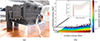 |
Figure 1 (a) The ICARE_NG2 flight model for HB13F with the sensors on the left of the instrument and the electronic box on the right. (b) Electron response function of the PE2 detection head aboard HB13F in anticoincidence mode. The inserted image corresponds to cross-sections of the response function, showing geometric factors as a function of incident energy. These geometric factors correspond to those actually used for count-flux conversions, as described in the next section. |
Various ranges of deposited energy were quantified during ground calibrations (Caron et al., 2024):
-
PE1: 300 keV to 6.3 MeV.
-
PE2: 420 keV to 8.8 MeV.
-
P2LE: 360 keV to 11.7 MeV.
The upper limits are directly driven by SSD thicknesses while the lower limits are driven by instrumental noise levels measured during ground calibrations. In addition, the gain of the charge amplifier also drives this energy range. However, in GEO, the instrument operates at relatively high temperatures (50 °C or higher), resulting in increased noise levels. For instance, at such temperatures, the lower limit for deposited energy in the PE2 detection head is about 600 keV.
For modeling the sensitivity of the different detection heads, their response functions have been simulated using GEANT4 (v10.3 patch 01). GEANT4 (Agostinelli et al., 2003; Allison et al., 2006) is a toolkit for the simulation of the passage of particles through matter. For both missions, the geometries of the satellites were provided by ADS (Airbus Defense and Space) in a degraded representation. The geometry of the satellite has been simplified into a sector-shielding analysis (ray-tracing). This approach produces distributions of shielding thickness as viewed from the center of the three detection heads as a function of direction from these locations. Incident particles were launched in all directions from any point outside the spacecraft (assuming isotropic fluxes), with different energies. All the deposited energies in the SSDs are then recorded. The geometric factors are calculated according to equation (1) (Sullivan, 1971) (1)where R is the radius of the source of particles, Ndet and Ntot are respectively the number of particles detected in the SSD(s) and the total number of particles launched from the source.
Figure 1b presents the Electron Response Function (ERF) of the PE2 for the anticoincidence acquisition mode. The inserted image corresponds to cross-sections of the ERF, showing geometric factors associated with specific channels (equivalent to a given deposited energy). In our case, these channels are the first ten usable channels, located above the instrument noise. Combined with the outputs of the instrument, it is then possible to deduce electron fluxes. The following section explains the process we used to do this.
3 Inversion methods
The instrument returns a histogram (counts) of the energies deposited in the SSDs. The relation between these counts and the associated particle fluxes is given by the Fredholm integral equation of the first kind (2)
(2)
Thus, based on the histogram of deposited energies, we want to reconstruct the corresponding particle fluxes as a function of incident energies. An inversion is consequently needed but this equation is a typical example of an ill-posed problem. Therefore, its solution is not guaranteed to be unique, nor a continuous function of the counts C. To calculate an approximate solution, two methods are detailed in the next part of this paper.
Both proposed inversion methods require a virtual electron flux database. Several sources can be used to create this database:
-
Specification models.
-
Analytical functions.
-
Fluxes observed by other instruments.
To ensure a wide variety of potential flux shapes, the database we have built is based on all the points mentioned above.
There are several specification models to describe particle fluxes in the Earth’s radiation belts. The most commonly used are AP8/AE8 (Sawyer & Vette, 1976; Vette, 1991) and AP9/AE9 (O’Brien et al., 2018) which provide an estimated of fluxes, everywhere in the radiation belts. Some models are also dedicated to certain regions as OPAL (Boscher et al., 2014b) and IGE (Sicard et al., 2019) and/or under specific conditions. In addition, the GREEN model (Sicard et al., 2019) combines AEX/APX and region-specific models to improve flux predictions. To build our electron flux database, AE8, AE9, and GREEN models were used. In addition, several spectra were randomly extracted from the electron fluxes measured on the EDRS-C mission. Finally, the exponential cut-off power law analytical function was selected (Aminalragia-Giamini et al., 2018) to complete the database (3)where a relates the intensity of the spectrum and b and c relate the power law and the exponential contribution. This function provides a means to combine spectra that have been well-identified in the literature. Parameter ranges of equation (3) are chosen to cover and extend the envelope of fluxes already defined. An extraction of the total database is shown Figure 2.
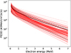 |
Figure 2 Omnidirectional differential fluxes of electrons (FEDO) as a function of incident electron energy. One thousand randomly selected spectra in our database. The solid black curve is the median of the distribution, and the dashed gray curves above and below are the 90th and 10th percentiles, respectively. |
3.1 Minimization by sensitivity analysis
In the context of mission preparation, sensitivity analysis, also known as Bowtie method (Boudouridis et al., 2020), of usable channels or groups of channels of a radiation monitor is a very good way to estimate instrument performance. Equations (4) and (5) provide the link between geometric factor (GI and GdE for integrated and differential factors respectively) and sensitive energy (ET and Eeff for threshold energy and effective energy respectively). (4)
(4)
 (5)
(5)
From these relations and our virtual electron fluxes database, it is possible to construct matrices, binned as (GI, ET) and (GdE, Eeff), to determine the best conversion parameter pairs. Figure 3a is the traditional representation of the Bowtie method. Figure 3b is an equivalent representation but the error for each pair of parameters is calculated. The procedure to generate such a matrix is as follows:
-
Channel or group of channels are selected.
-
Virtual fluxes are injected into equation (2) to obtain virtual counts.
-
Each pair of conversion parameters is used with the selected channel or group of channels to estimate the corresponding flux.
-
The error between the estimated flux and the expected flux is calculated.
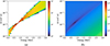 |
Figure 3 (a) Binned Bowtie representation of channel 10 of the PE2 detection head aboard HB13F using (4). The colorscale corresponds to the contribution of the database measurements used in relation to the grid’s (GI, ET) pairs. (b) Binned error map (based on the 75th of the error distribution) representation of channel 10 of the PE2 detection head aboard HB13F using (4). The color scale corresponds to the error evaluation. |
The error then calculated is for each sample of the database. Consequently, it is therefore possible to build up an error distribution for the whole database. In this way, a matrix Merr of dimension m × n × p is constructed where m and n are the number of bins used to build the conversion parameters using (4) or (5) and p is the number of samples in the database. Figure 3b corresponds to Merr using the 75th percentile of the error distribution in the case of channel 10 of PE2 aboard HB13F.
Optimal conversion parameters can then be extracted either by taking a unique pair that minimizes the error or by setting a tolerated error threshold. Figure 4 presents the results extracted from the matrix displayed in Figure 3b, with a maximum error tolerance of 15%.
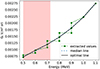 |
Figure 4 Conversion parameters extracted from the matrix shown in Figure 3b, combined with a 15% error tolerance. Green squares are directly extracted from the matrix, the blue dashed line corresponds to the median y-values and the black line corresponds to the optimal line (keeping only the minimal error for each energy). The red zone corresponds to non-physical sensitivity. |
Such results can be misleading, as energies lower than the monitor’s intrinsic sensitivity can be identified as parameters. Indeed, channel 10 of the PE2 detection head aboard HB13F corresponds to a deposited energy of ∼700 keV. Of course, no electron of less than 700 keV can deposit such energy. Consequently, it is not possible to keep conversion parameters associated with energies lower than those allowed by the selected channel. Otherwise, this is equivalent to extrapolating the sensitivity of a higher energy thanks to the database.
3.2 Complete minimization
The complete minimization method considers expected shapes as written in equation (3) and can be written as equation (6)
 (6)where C is the real count of the instruments. This second method is therefore totally independent of the first one since the results of the Bowtie method are not used as additional constraints to the minimization. The three parameters (a, b, c) are optimized to minimize the reconstruction error of the counts observed by the instruments. The reconstruction error is then calculated, providing a warning of any significant deviation (typically when the average error is greater than 20%). Unlike the sensitivity analysis method, complete minimization offers a straightforward way to quantify the quality of the conversion performed. The validity domain of the conversion is also verified by reducing the incident energy window of the response functions. The influence of the lowest and the highest incident energies on the count’s reconstructions are calculated in relation to a reconstruction performed over the entire incident energy domain of the response functions. As long as the reduction of the lowest and highest incident energies does not modify the conversion error, these energies are considered as non-relevant. This approach reveals the area of incident energy involved in the measurement.
4 Results and comparisons
4.1 Inversion methods comparison
A good way to validate the conversion of the instrument’s measurements to fluxes is to use different inversion methods and compare their results. While the minimization by sensitivity analysis considered only virtual counts, the complete minimization method uses real counts. The comparison of the two approaches is therefore well justified. Figure 5a shows a comparison based on ICARE_NG2 data averaged over April 1, 2024 day. Figure 5b shows the reconstruction performance of the corresponding count rates.
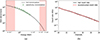 |
Figure 5 (a) Electron integral fluxes as a function of incident electron energy. Comparison of the two inversion methods described in the paper. The black curve corresponds to the full minimization method while the green dots with error bars correspond to the sensitivity analysis method. The calculated fluxes correspond to the day of 2023-04-01 observed by HotBird missions. In the case of inversion by sensitivity analysis, some energies are covered by different channels, which explains the overlap of some error bars. The red zones correspond to energies that have no influence, or very limited influence, on the instrument’s measurements. (b) Count rates observed (black full line) and reconstructed (red dashed line) during the same day. |
Both methods are in excellent agreement. An average error of less than 5% is obtained with the complete minimization on the count reconstructions. The comparison was performed over a wide time interval and no significant deviations were observed. The main difficulty with the complete minimization method is dealing with very low counts, where statistical fluctuations are significant. Two simple solutions are then possible to ensure the continuity of the results, averaging the counts over a longer integration time or switching to the first inversion method.
4.2 Comparison with EDRS-C/NGRM
NGRM is the second Space Weather instrument flying as part of ESA’s Distributed Space Weather Sensor System (D3S). One of the NGRM units was placed on the GEO European Data Relay System – C (EDRS-C) spacecraft (Sandberg et al., 2022). The instrument provides electron differential fluxes, also called FEDO (Omnidirectionnal Differential Electron Fluxes), and electron integral fluxes, also called FEIO (Omnidirectionnal Integrated Electron Fluxes), re-calibrated using electron flux measurements from Arase mission (Higashio et al., 2018). The instrument measurements are available on https://swe.ssa.esa.int/sparc-geo-ngrm-r170-federated. Figures 6a and 6b compare electron fluxes measured by ICARE_NG2 and NGRM. Figure 6a proposes a time series comparison with ICARE_NG2 observations averaged every minute, as are NGRM data. The selected energies are close enough from one instrument to the other to be comparable, and the associated fluxes are expected to be very similar. Figure 6b shows the average electron flux for all the energies measured by the instruments over the same time period.
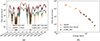 |
Figure 6 (a) Time series of electron fluxes measured by ICARE_NG2 aboard HB13G and NGRM aboard EDRS-C. For each missions two energies are considered: 600 keV and 1.2 MeV for NGRM and 650 keV and 1.3 MeV for ICARE_NG2. These energies have been chosen close enough between the two instruments to be directly comparable. (b) Comparison of electron integral fluxes given by ICARE_NG2 and NGRM instruments as a function of incident electron energies. The same time slot as (a) is used and averaged for each available energy. The orange solid line corresponds to the transformation of FEDO to FEIO provided by NGRM. |
Both instruments provide very similar observations, not only in absolute values but also dynamically. As the outer belt is particularly dynamic, and directly driven by the solar activity, variations of several orders of magnitude can be observed for the same incident energy. ICARE_NG2 measurements are substantially noisier than those of NGRM. This is due to the size of the SSDs used, which have been optimized for the EOR phase of the missions (for limiting saturation issues). The spectra provided by the two instruments are also in very good agreement (see Fig. 6b). As NGRM gives FEIO only up to 1.2 MeV, FEDO have been integrated to obtain higher energies. The highest available energies (2.9, 3.4, and 4 MeV) are not presented here, as the relevance of their integration results is no longer truly representative.
4.3 Comparison with specification models
Another important comparison is to evaluate the specification models commonly used for radiation qualification of space missions. AE8, AE9, and IGE will thus be compared with the observations of the ICARE_NG2 instruments, as presented in Figure 7. The aforementioned specification models provide flux estimates obtained essentially empirically, with a statistical approach to several datasets. As these are long-term models, several months (at least) of ICARE_NG2 instrument measurements should be averaged for comparison purposes.
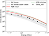 |
Figure 7 Comparisons of ICARE_NG2 measurements with several specification models: green full line, red full line, and gray dashed line for AE9 mean, AE8 and IGE models respectively. In GEO, AE8 provides the same results at both minimum and maximum solar activity. Lower and upper cases for IGE model are also indicated by the gray area. |
AE8 and AE9 mean models provide very similar results in the targeted energy range. However, IGE mean model offers estimates that are a factor of 3–4 below those predicted by the AE8 and AE9 mean models. ICARE_NG2 observations fall between the three models, while being relatively close to the IGE mean estimations. There is a factor of about 2 between the observations and the estimations of AE8 and AE9 mean models, whereas the distribution of the IGE model given by the upper and lower cases fully integrates the measures. These conclusions are in line with (Caron et al., 2022).
5 GEO model for daily electron fluxes
Using GEO observations (given by ICARE_NG2 and NGRM instruments especially), we have developed a fully analytical model in order to restituate the daily fluxes observed by the instruments. In addition to specification models such as IGE which provide long-term predictions, several models propose simplified approaches to describe electron dynamics in GEO. Li et al. (2001) and Li (2004) have developed a 1D radial diffusion equation using solar wind data to change the radial diffusion rate. Katsavrias et al. (2021) have developed a multiple regression model, using also solar wind data and providing an analytical expression of the electron fluxes. Boynton et al. (2015) and Landis et al. (2022) use Recurrent Neural Network (RNN) based on Geostationary Operational Environmental Satellite (GOES) measurements to train their models. The advantage of our approach compared to existing models is that a limited number of parameters are used while offering electron energy dependency.
First, a shape function, g, is established including solar wind velocity, the z-component of the interplanetary magnetic field (IMF) in GSM coordinates, and the magnetopause standoff distance, calculated with the Shue model (Shue et al., 1998). The shape function is designed to align with the dynamics of the fluxes, while an additional function, referred to as the transformation function, T, is required to map the shape function’s results into the flux domain, thereby yielding the adjusted absolute values. The shape function is given by equation (7)
 (7)the third term is based on Li et al. (2001) who suggest a dependence of electron fluxes with the y-component of solar wind electric field. Figure 8 presents all these ingredients during the first half of 2022. The NGRM measurements for the same period are also displayed to visually highlight the correlations with electron fluxes.
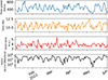 |
Figure 8 Solar wind data used in the proposed model. The first plot corresponds to the solar wind speed, the second one corresponds to the magnetopause location using the Shue model, the third one corresponds to the last term of g(t) and the last plot is the observations of 600 keV electrons provided by EDRS-C/NGRM. The first half of 2022 is presented. |
 and
and  are the averaged values of the solar wind velocity and the magnetopause standoff distance respectively over the considered period. The six parameters of the shape function g(t) are optimized using a few months of observations (see Fig. 9a). The predicted results were compared to the observations by minimizing χ2:
 (8)
(8)
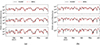 |
Figure 9 Model predictions compared to EDRS-C/NGRM observations for three different electron energies: 180 keV (top panels), 600 keV (middle panels), and 1.3 MeV (bottom panels). (a) and (b) are periods used to optimize and validate the six parameters of the shape function g(t). |
No energy dependency was evident from the determination of these parameters and a single set was thus obtained: c1 = 0.00065, γ1 = 2, c2 = 170, γ2 = 0.15, c3 = 1, γ3 = 2. In the considered case (see Fig. 8),  km/s and
  Re. It should be noted, however, that the minimization of χ2 becomes increasingly poor as higher-energy electrons are considered. Whereas at energies below 1 MeV, χ2 is less than 0.1, for higher energies (up to 4 MeV), it reaches 0.3. This is due to the formulation of g(t) which is driven exclusively by solar wind parameters. Very high-energy electrons come mainly from acceleration processes within the radiation belts. These phenomena are not directly captured by the established expression of g(t). However, it is initially the low-energy electrons that are accelerated, and since our approach focuses on daily fluxes, the general trend is well retained by the model (see Figs. 9a and 9b).
Transformation function T(E) is needed to project the g(t) values into electron flux space. This function makes the link between the percentile distributions of g(t) and the observed electron fluxes. For each incident energy, the transformation function is calculated to reveal energy dependency. Figure 10a presents the relation between g(t) and observations percentiles. Figures 10b and 10c correspond to the extracted parameters of the fitted lines in Figure 10a.
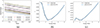 |
Figure 10 Plots of the various elements of the transformation function. (a) Relations between percentile distributions of g(t) and the observations. The dashed lines are linear fits for each electron energy of the EDRS-C/NGRM instrument. (b) and (c) are the coefficients of the linear fits as a function of the electron energies. The dashed blue lines are polynomial fits. |
Polynomial fits are proposed in Figures 10b and 10c in order to fully formalize an analytical writing of our expression. Equations (9) and (10) express these two terms (9)
(9)
 (10)and finally, the complete expression is given by equation (11)
 (11)
(11)
The model developed provides very good reconstructions of ICARE_NG2 and NGRM daily observations. Good predictions can then be expected over longer averaged timescales. Figure 11 presents four time periods where observations are averaged: 3, 6, 12, and 24 months. Average electron flux dynamics vary slightly over the entire observed period, with a maximum factor of 3, which is well reflected in the model.
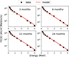 |
Figure 11 Averaged electron fluxes estimations (red full lines) compared to EDRS-C/NGRM observations (black squares). As indicated on the plots, four cases are considered: averaged over 3, 6, 12, and 24 months. |
It should be noted, however, that our approach does not take the solar cycle into account. A dependence on the F10.7 index or a cosine law, for instance, will have to be considered to exploit our model over much longer time periods. This aspect is not observable on the data used and is therefore not included in the current development of the model.
6 Conclusions
Two ICARE_NG2 radiation monitors are now in geostationary orbit on the HB13F and HB13G missions. Both instruments have the same detection heads and present identical observations. Measurements of electrons from 650 keV to 2 MeV in GEO are now available and will be distributed on https://swe.ssa.esa.int/icare-ng. Two inversion methods were presented, and the limitations of each were discussed. The associated results were compared, as well as with measurements from the NGRM radiation monitor aboard the EDRS-C spacecraft. Excellent agreement was observed, with no need for cross-calibration. Due to the good performance observed and the simplicity of use, the fluxes distributed on the ESA website are derived using the Bowtie method. The use of observations now available in GEO has also driven the development of an analytical model providing daily electron fluxes as a function of electron energies and solar wind data. Despite its simplicity, the model can reproduce both the dynamics and intensities of the electron fluxes. However, the dynamics of very high-energy electrons (above 2 MeV) are not as well reproduced as for low-energy electrons. In addition, the expected modulation of fluxes by the solar cycle is not considered. These points may be the aim of a dedicated study in the future.
Acknowledgments
The editor thanks Xinlin Li and an anonymous reviewer for their assistance in evaluating this paper.
References
- Agostinelli S, Allison J, Amako K, Apostolakis J, Araujo H, et al. 2003. Geant4 – simulation toolkit. Nucl Instrum Methods Phys Res A 506(3): 250–303. https://doi.org/10.1016/S0168-9002(03)01368-8. [CrossRef] [Google Scholar]
- Allison J, Amako K, Apostolakis J, Araujo H, Arce Dubois P, et al. 2006. Geant4 developments and applications. IEEE Trans Nucl Sci 53(1): 270–278. https://doi.org/10.1109/TNS.2006.869826. [CrossRef] [Google Scholar]
- Aminalragia-Giamini S, Papadimitriou C, Sandberg I, Tsigkanos A, Jiggens P, Evans H, Rodgers D, Daglis IA. 2018. Artificial intelligence unfolding for space radiation monitor data. J Space Weather Space Clim 8: A50. https://doi.org/10.1051/swsc/2018041. [CrossRef] [EDP Sciences] [Google Scholar]
- Boscher D, Bourdarie SA, Falguere D, Lazaro D, Bourdoux P, Baldran T, Rolland G, Lorfevre E, Ecoffet R. 2011. In flight measurements of radiation environment on board the french satellite JASON-2. IEEE Trans Nucl Sci 58(3): 916–922. https://doi.org/10.1109/TNS.2011.2106513. [CrossRef] [Google Scholar]
- Boscher D, Cayton T, Maget V, Bourdarie S, Lazaro D, Baldran T, Bourdoux P, Lorfevre E, Rolland G, Ecoffet R. 2014a. In-flight measurements of radiation environment on board the argentinean satellite SAC-D. IEEE Trans Nucl Sci 61(6): 3395–3400. https://doi.org/10.1109/TNS.2014.2365212. [CrossRef] [Google Scholar]
- Boscher D, Sicard-Piet A, Lazaro D, Cayton T, Rolland G. 2014b. A new proton model for low altitude high energy specification. IEEE Trans Nucl Sci 61: 3401–3407. https://doi.org/10.1109/TNS.2014.2365214. [CrossRef] [Google Scholar]
- Boudouridis A, Rodriguez J, Kress B, Dichter B, Onsager T. 2020. Development of a bowtie inversion technique for real-time processing of the GOES-16/-17 SEISS MPS-HI electron channels. Space Weather 18(4): e2019SW002403. https://doi.org/10.1029/2019SW002403. [CrossRef] [Google Scholar]
- Boynton RJ, Balikhin MA, Billings SA. 2015. Online NARMAX Model for electron fluxes at GEO. Ann Geophys 33(3): 405–411. https://doi.org/10.5194/angeo-33-405-2015. [CrossRef] [Google Scholar]
- Caron P, Bourdarie S, Falguère D, Lazaro D, Bourdoux P, et al. 2022. In-flight measurements of radiation environment observed by Eutelsat 7C (electric orbit raising satellite). IEEE Trans Nucl Sci 69(7): 1527–1532. https://doi.org/10.1109/TNS.2022.3158470. [CrossRef] [Google Scholar]
- Caron P, Bourdarie S, Sicard A, Carron J, Calaprice M, et al. 2024. In-flight measurements of radiation environment observed by Hotbird 13F and Hotbird 13G (electric orbit raising satellites). IEEE Trans Nucl Sci 71: 1535–1541. https://doi.org/10.1109/TNS.2024.3367730. [CrossRef] [Google Scholar]
- Caron P, Inguimbert C, Artola L, Chatry N, Sukhaseum N, Ecoffet R, Bezerra F. 2018. Physical mechanisms inducing electron single-event upset. IEEE Tran Nucl Sci 65(8): 1759–1767. https://doi.org/10.1109/TNS.2018.2819421. [CrossRef] [Google Scholar]
- Caron P, Inguimbert C, Artola L, Ecoffet R, Bezerra F. 2019. Physical mechanisms of proton-induced single-event upset in integrated memory devices. IEEE Trans Nucl Sci 66(7): 1404–1409. https://doi.org/10.1109/TNS.2019.2902758. [CrossRef] [Google Scholar]
- Higashio N, Takashima T, Shinohara I, Matsumoto H. 2018. The extremely high-energy electron experiment (XEP) onboard the arase (ERG) satellite. Earth Planet Space 70(1): 134. https://doi.org/10.1186/s40623-018-0901-x. [CrossRef] [Google Scholar]
- Katsavrias C, Aminalragia-Giamini S, Papadimitriou C, Sandberg I, Jiggens P, Daglis I, Evans H. 2021. On the interplanetary parameter schemes which drive the variability of the source/seed electron population at GEO. J Geophys Res Space Phys 126(6): e2020JA028939. https://doi.org/10.1029/2020JA028939. [CrossRef] [Google Scholar]
- Landis DA, Saikin AA, Zhelavskaya I, Drozdov AY, Aseev N, Shprits YY, Pfitzer MF, Smirnov AG. 2022. NARX neural network derivations of the outer boundary radiation belt electron flux. Space Weather 20(5): e2021SW002774. https://doi.org/10.1029/2021SW002774. [CrossRef] [Google Scholar]
- Li X. 2004. Variations of 0.7–6.0 MeV electrons at geosynchronous orbit as a function of solar wind. Space Weather 2(3): S03006. https://doi.org/10.1029/2003SW000017. [Google Scholar]
- Li X, Temerin M, Baker DN, Reeves GD, Larson D. 2001. Quantitative prediction of radiation belt electrons at geostationary orbit based on solar wind measurements. Geophys Res Lett 28(9): 1887–1890. https://doi.org/10.1029/2000GL012681. [CrossRef] [Google Scholar]
- Matéo-Vélez J-C, Sicard A, Payan D, Ganushkina N, Meredith NP, Sillanpäa I. 2018. Spacecraft surface charging induced by severe environments at geosynchronous orbit. Space Weather 16(1): 89–106. https://doi.org/10.1002/2017SW001689. [CrossRef] [Google Scholar]
- Messenger SR, Wong F, Hoang B, Cress CD, Walters RJ, Kluever CA, Jones G. 2014. Low-thrust geostationary transfer orbit (LT2GEO) radiation environment and associated solar array degradation modeling and ground testing. IEEE Trans Nucl Sci 61(6): 3348–3355. https://doi.org/10.1109/TNS.2014.2364894. [CrossRef] [Google Scholar]
- O’Brien TP, Johnston WR, Huston SL, Roth CJ, Guild TB, Su Y-J, Quinn RA. 2018. Changes in AE9/AP9-IRENE version 1.5. IEEE Trans Nucl Sci 65(1): 462–466. https://doi.org/10.1109/TNS.2017.2771324. [CrossRef] [Google Scholar]
- Sandberg I, Aminalragia-Giamini S, Papadimitriou C, Van Gijlswijk R, Heynderickx D, Marcinkowski R, Hajdas W, Heil M, Evans H. 2022. First results and analysis from ESA next generation radiation monitor unit onboard EDRS-C. IEEE Trans Nucl Sci 69(7): 1549–1556. https://doi.org/10.1109/TNS.2022.3160108. [CrossRef] [Google Scholar]
- Sawyer DM, Vette JI. 1976. AP-8 Trapped proton environment for solar maximum and solar minimum. National Space Science Data Center (NSSDC), World Data Center A for Rockets and Satellites (WDC-A-R&S). [Google Scholar]
- Shue J-H, Song P, Russell CT, Steinberg JT, Chao JK, et al. 1998. Magnetopause location under extreme solar wind conditions. J Geophys Res Space Phys 103(A8): 17691–17700. https://doi.org/10.1029/98JA01103. [CrossRef] [Google Scholar]
- Sicard A, Boscher D, Lazaro D, Bourdarie S, Standarovski D, Ecoffet R. 2019. New model for the plasma electrons fluxes (part of GREEN model). IEEE Trans Nucl Sci 66(7): 1738–1745. https://doi.org/10.1109/TNS.2019.2923005. [CrossRef] [Google Scholar]
- Sullivan JD. 1971. Geometric factor and directional response of single and multi-element particle telescopes. Nucl Instrum Methods 95(1): 5–11. https://doi.org/10.1016/0029-554X(71)90033-4. [CrossRef] [Google Scholar]
- Van Allen JA, Frank LA. 1959. Radiation around the earth to a radial distance of 107,400 km. Nature 183(4659): 430–434. https://doi.org/10.1038/183430a0. [CrossRef] [Google Scholar]
- Vette JI. 1991. The AE-8 trapped electron model environment. National Space Science Data Center (NSSDC), World Data Center A for Rockets and Satellites (WDC-A-R&S), National Aeronautics and Space Administration, Goddard Space Flight Center. [Google Scholar]
Cite this article as: Caron P, Bourdarie S, Carron J, Ecoffet R, Terzo S, et al. 2025. Geostationary electron dynamics: ICARE_NG2 observations and new analytical model of daily electron fluxes driven by solar wind conditions. J. Space Weather Space Clim. 15, 18. https://doi.org/10.1051/swsc/2025017.
All Figures
|
Figure 1 (a) The ICARE_NG2 flight model for HB13F with the sensors on the left of the instrument and the electronic box on the right. (b) Electron response function of the PE2 detection head aboard HB13F in anticoincidence mode. The inserted image corresponds to cross-sections of the response function, showing geometric factors as a function of incident energy. These geometric factors correspond to those actually used for count-flux conversions, as described in the next section. |
| In the text | |
|
Figure 2 Omnidirectional differential fluxes of electrons (FEDO) as a function of incident electron energy. One thousand randomly selected spectra in our database. The solid black curve is the median of the distribution, and the dashed gray curves above and below are the 90th and 10th percentiles, respectively. |
| In the text | |
|
Figure 3 (a) Binned Bowtie representation of channel 10 of the PE2 detection head aboard HB13F using (4). The colorscale corresponds to the contribution of the database measurements used in relation to the grid’s (GI, ET) pairs. (b) Binned error map (based on the 75th of the error distribution) representation of channel 10 of the PE2 detection head aboard HB13F using (4). The color scale corresponds to the error evaluation. |
| In the text | |
|
Figure 4 Conversion parameters extracted from the matrix shown in Figure 3b, combined with a 15% error tolerance. Green squares are directly extracted from the matrix, the blue dashed line corresponds to the median y-values and the black line corresponds to the optimal line (keeping only the minimal error for each energy). The red zone corresponds to non-physical sensitivity. |
| In the text | |
|
Figure 5 (a) Electron integral fluxes as a function of incident electron energy. Comparison of the two inversion methods described in the paper. The black curve corresponds to the full minimization method while the green dots with error bars correspond to the sensitivity analysis method. The calculated fluxes correspond to the day of 2023-04-01 observed by HotBird missions. In the case of inversion by sensitivity analysis, some energies are covered by different channels, which explains the overlap of some error bars. The red zones correspond to energies that have no influence, or very limited influence, on the instrument’s measurements. (b) Count rates observed (black full line) and reconstructed (red dashed line) during the same day. |
| In the text | |
|
Figure 6 (a) Time series of electron fluxes measured by ICARE_NG2 aboard HB13G and NGRM aboard EDRS-C. For each missions two energies are considered: 600 keV and 1.2 MeV for NGRM and 650 keV and 1.3 MeV for ICARE_NG2. These energies have been chosen close enough between the two instruments to be directly comparable. (b) Comparison of electron integral fluxes given by ICARE_NG2 and NGRM instruments as a function of incident electron energies. The same time slot as (a) is used and averaged for each available energy. The orange solid line corresponds to the transformation of FEDO to FEIO provided by NGRM. |
| In the text | |
|
Figure 7 Comparisons of ICARE_NG2 measurements with several specification models: green full line, red full line, and gray dashed line for AE9 mean, AE8 and IGE models respectively. In GEO, AE8 provides the same results at both minimum and maximum solar activity. Lower and upper cases for IGE model are also indicated by the gray area. |
| In the text | |
|
Figure 8 Solar wind data used in the proposed model. The first plot corresponds to the solar wind speed, the second one corresponds to the magnetopause location using the Shue model, the third one corresponds to the last term of g(t) and the last plot is the observations of 600 keV electrons provided by EDRS-C/NGRM. The first half of 2022 is presented. |
| In the text | |
|
Figure 9 Model predictions compared to EDRS-C/NGRM observations for three different electron energies: 180 keV (top panels), 600 keV (middle panels), and 1.3 MeV (bottom panels). (a) and (b) are periods used to optimize and validate the six parameters of the shape function g(t). |
| In the text | |
|
Figure 10 Plots of the various elements of the transformation function. (a) Relations between percentile distributions of g(t) and the observations. The dashed lines are linear fits for each electron energy of the EDRS-C/NGRM instrument. (b) and (c) are the coefficients of the linear fits as a function of the electron energies. The dashed blue lines are polynomial fits. |
| In the text | |
|
Figure 11 Averaged electron fluxes estimations (red full lines) compared to EDRS-C/NGRM observations (black squares). As indicated on the plots, four cases are considered: averaged over 3, 6, 12, and 24 months. |
| In the text | |
Current usage metrics show cumulative count of Article Views (full-text article views including HTML views, PDF and ePub downloads, according to the available data) and Abstracts Views on Vision4Press platform.
Data correspond to usage on the plateform after 2015. The current usage metrics is available 48-96 hours after online publication and is updated daily on week days.
Initial download of the metrics may take a while.