| Issue |
J. Space Weather Space Clim.
Volume 15, 2025
Topical Issue - Swarm 10-Year Anniversary
|
|
|---|---|---|
| Article Number | 30 | |
| Number of page(s) | 19 | |
| DOI | https://doi.org/10.1051/swsc/2025026 | |
| Published online | 18 July 2025 | |
Research Article
Intermittency in the integrated power of ionospheric density fluctuations
1
Department of Physics and Astronomy, University of Calgary, T2N 1N4 Calgary, Alberta, Canada
2
Institute for Astronomy, Astrophysics, Space Applications and Remote Sensing, National Observatory of Athens, 15236 Athens, Greece
3
Department of Geomatics Engineering, University of Calgary, T2N 1N4 Calgary, Alberta, Canada
* Corresponding author: This email address is being protected from spambots. You need JavaScript enabled to view it.
Received:
27
November
2024
Accepted:
29
May
2025
Abstract
The occurrence of ionospheric irregularities poses a significant challenge to Global Navigation Satellite Systems (GNSS) by disrupting signal propagation and causing loss of lock (LOL) events. This study investigates the integrated power spectral density (PSD) of electron density fluctuations at various scales using nearly ten years of Swarm satellite data. The analysis focuses on the post-sunset equatorial ionosphere, a region prone to ionospheric irregularities. GPS receivers on Swarm A and C, orbiting at altitudes between 430 and 460 km, suffer more frequent loss of navigational capability (LNC) than Swarm B (at 530 km). The observed power-law distribution of integrated power at small spatial scales (<30 km) points to scale-free behavior, which is a hallmark of complex systems and may be associated with self-organized criticality (SOC). The study also employs multifractal detrended fluctuation analysis (MFDFA) to demonstrate the multifractal and intermittent nature of the fluctuations. The findings highlight the importance of intermittency and strong bursts in understanding the LNC and LOL events in the ionosphere. This research contributes to a deeper understanding of the dynamics of ionospheric irregularities and offers potential for improved forecasting and mitigation of their impact on GNSS.
Key words: Self-organized criticality / Intermittency / Ionospheric irregularity
Publisher note: The title was changed from "Intermittency in the integrated power ofionospheric density fluctuations" to "Intermittency in the integrated power of ionospheric density fluctuations" on 24 July 2025.
© H. Ghadjari et al., Published by EDP Sciences 2025
 This is an Open Access article distributed under the terms of the Creative Commons Attribution License (https://creativecommons.org/licenses/by/4.0), which permits unrestricted use, distribution, and reproduction in any medium, provided the original work is properly cited.
1 Introduction
One of the significant challenges in positioning and navigation using the Global Navigational Satellite System (GNSS) arises from the presence of ionospheric irregularities (Meecham, 1964; Yeh et al., 1975; Klobuchar, 1983; Bishop et al., 1990). These irregularities can lead to a reduction in measurement precision for pseudorange and carrier phase measurements. The ionosphere’s plasma density structures can disrupt the propagation of electromagnetic signals, causing Loss of Lock (LOL) events where GNSS receivers fail to acquire the signal from one or more GNSS satellites (Xiong et al., 2016; Pezzopane et al., 2021; De Michelis et al., 2022). Xiong et al. (2016) refer to the complete disruption of signals from all visible satellites as total LOL. Ionospheric irregularities are regularly observed in the post-sunset equatorial and high-latitude ionospheres.
Field-aligned plasma bubbles represent a class of ionospheric irregularity occurring within the post-sunset equatorial ionosphere and typically observed in conjugate hemispheres (McClure et al., 1977; Keskinen et al., 1998; Kil et al., 2009; Kil, 2015; Ghadjari et al., 2022). Ionospheric irregularities associated with polar cap patches and auroras are observed at high geomagnetic latitudes. According to Xiong et al. (2016), post-sunset ionospheric irregularities in the equatorial ionosphere occur in two bands between ±5° and ±20° magnetic latitude and were responsible for a significant share of the total LOL occurrences (96%) within the first two years of the Swarm mission. Plasma depletions in these instances were greater than 10 × 1010 m−3, and the background plasma density in these total LOL events is among the highest background plasma densities reported by the Swarm Langmuir probe (LP). Only less than 4% of the total LOL events occurred at high latitudes. The high-latitude events occurred mostly near local noon due to large density gradients compared to the background density in the auroral or polar cap regions (Fffihn Follestad et al., 2020). Most ionospheric irregularities are close to the Swarm’s altitudes, as shown by Zakharenkova et al. (2016). They compare the in-situ plasma density with total electron content (TEC) derived from the Swarm Global Positioning System (GPS) receivers.
Plasma instability processes with a high growth rate in the ionosphere can cause it to transition from a quiet state to a turbulent state. This turbulent state emerges from continuous instability processes (Tritton, 2012). One of these instability mechanisms is the Rayleigh-Taylor (R-T) instability. The R-T instability arises in the post-sunset equatorial ionosphere, where a steep upward-directed plasma density gradient forms due to rapid recombination in the E region. This unstable configuration, with a higher density plasma overlaying a lower density plasma, leads to equatorial plasma bubbles (EPB) that expand into the ionosphere, contributing to large-scale turbulence and GPS signal scintillation (Panda et al., 2019; Vankadara et al., 2023). To understand ionospheric turbulence, researchers have focused on studying the different scales of ionospheric irregularities and their relationship to the cascade process. For example, studies have shown that the R-T instability can generate irregularities spanning scales from meters to kilometers, which are critical to understanding the cascade of energy across different scales (Panda et al., 2019; Vankadara et al., 2023). Kintner & Seyler (1985) investigated the cascade of turbulence in the ionosphere and found similarities to fluid turbulence, where the energy cascade spectrum follows a power law in the inertial range (Frisch, 1980). The irregularity spectrum in the ionosphere, which describes the dependence of irregularities on wavenumbers, also exhibits a power-law shape (represented as a line in a log-log plot). This power-law behavior suggests the coexistence of intermediate-scale irregularities (on the order of kilometers) and small-scale irregularities down to hundreds of meters (Shkarofsky, 1968; Costa & Kelley, 1977; Kivanç & Heelis, 1998; Spicher et al., 2014). An alternative method to study scale sizes of irregularities and cascade process includes examining ionospheric irregularities by analyzing the power spectra of GPS signal intensity and phase measurements (Jayachandran et al., 2017; Song et al., 2021; Hamza et al., 2023; Mohandesi et al., 2024). In order to identify the fundamental instability mechanism that governs the cascade process, Kintner & Seyler (1985) emphasize the importance of studying the slope of the power spectra for both the plasma density and the electric field. The power spectra of the in situ plasma irregularity data and ground-based GPS carrier measurements were found to have similar slopes by Jin et al. (2019) in lower frequencies, indicating that in-situ data can be used to estimate GPS scintillation on the ground. In addition, the use of ground GPS data allows for ionospheric remote sensing.
Structure-function analysis provides a comprehensive approach to investigate ionospheric irregularity turbulence using in-situ data (De Michelis et al., 2021a, 2022; Ghadjari et al., 2023). The second-order scaling exponent obtained through structure-function analysis provides information comparable to that given by power spectrum methods but allows the investigation of turbulence drivers, intermittent behavior, and energy dispersion across multiple temporal and spatial scales.
Intermittency is a well-known phenomenon characterized by occasional or irregular bursts of intense activity within a turbulent flow (Hajj, 1999; Sreenivasan, 1999). It is observed in different regions of space plasma (Kivanç & Heelis, 1998; Chang, 1999; Sorriso-Valvo et al., 1999; Consolini & Chang, 2002; Lui, 2002; Chang et al., 2004; Spicher et al., 2014). The idea of intermittency was initially discovered by Batchelor & Townsend (1949) through the observation that successive time derivatives of a turbulent signal became more bursty at higher derivative orders. This phenomenon is dominant at smaller scales within the turbulence dissipation range; however, McComb & May (2018) state that in the most recent definition of intermittency, this phenomenon can be studied at all scale sizes, not just small-scale structures in turbulent states. It is important to note that intermittency is sometimes associated with heavy-tailed distributions, where rare or extreme events that significantly deviate from the average occur more commonly (Bryson, 1974; Pisarenko & Rodkin, 2010; Cooke & Nieboer, 2011). Intermittency is unlikely in a series of events that follow a Gaussian distribution (Iliopoulos et al., 2012).
Understanding the physical picture of an intermittent event is crucial. The wavelet transform of turbulence structures allows for the separation of structures within a turbulent medium according to their nature: random or coherent (Hussain, 1986; Farge, 1992; Spicher et al., 2015). In a magnetized plasma, coherent structures, such as “field-aligned magnetic flux tubes, current filaments, stationary structures, and convective structures,” exhibit longer average lifetimes compared to random structures, as noted by Chang et al. (2010). The stochastic interaction of coherent structures at all scales causes intermittent fluctuations. These intermittent fluctuations coexist with a sea of random background structures, the intensity of which exhibits a Gaussian distribution. In the specific case of ionospheric irregularities, coherent structures have been studied at high latitudes by Spicher et al. (2015) and in the post-sunset equatorial ionosphere by Chian et al. (2018).
It is difficult to study the intermittency at the level of individual events. Statistical methods are commonly employed to analyze intermittency and gain insights into its nature. Two prominent methods in this regard are structure-function analysis and multifractality analysis (Schertzer & Lovejoy, 1985; Lovejoy & Schertzer, 1991; Dudok de Wit & Krasnosel’skikh, 1996; Robert, 1996; Tessier et al., 1996; Consolini et al., 2020; Balasis et al., 2023a; Meziane et al., 2023). Structure-function analysis involves calculating the moments or statistical quantities at different lag distances or scales. In intermittent phenomena, the scaling exponents may exhibit non-linear behavior, such as increasing or decreasing with the lag distances. These anomalous scaling exponents reflect the intermittent nature of the underlying data (Dyrud et al., 2008; De Michelis et al., 2021a). Multifractality explores the relationship between fluctuations at different scale sizes within a dataset. Fluctuations in the data are characterized by their strength or magnitude at each scale size. Intermittency is manifested by irregular bursts or occasional events of intense activity within the data. These bursts are associated with localized regions or structures that deviate significantly from the average behavior (Chang et al., 2010; Calif et al., 2013). Fractal and multifractal analysis serves not only as a means to reveal intermittency within the system but also as a powerful tool to unveil the underlying complexity (Ivanov et al., 1999; Shimizu et al., 2002; Balasis et al., 2006; Balasis et al., 2023a, b; Sen, 2007). Another method for studying intermittency is the Local Intermittency Measure (LIM). This method has been performed on sounding rocket data to study winter cusp ionospheric irregularities by Di Mare et al. (2021). They suggested that this method can be applied to plasma density data to find different drivers of turbulence of ionospheric irregularities.
The connection between the Swarm GPS device’s LOL events and the scaling exponents of structure-function analysis of plasma density fluctuations has been investigated by De Michelis et al. (2022). They discovered that turbulent metrics, such as the existence of intermittent structures and a relatively high rate of change of the electron density index (RODI) values, can be utilized to differentiate between turbulent plasma densities, which lead to GPS LOL, and weaker turbulence structures. Another study by De Michelis et al. (2021a) focuses on the structure-function analysis of electron density fluctuations in the mid-latitude and high-latitude ionosphere, utilizing the down-sampled Swarm LP data. Their investigation identifies two distinct sets of plasma density fluctuations, one in the auroral zone in the high-latitude ionosphere and the other at middle latitudes, with differing spectral exponents and RODI values. The population within the auroral oval exhibits a spectral exponent of 1.7, while the second population at middle latitudes shows a spectral exponent of 2 or higher. These spectral exponents in auroral oval irregularities align with other observations and theoretical predictions of irregularities caused by gradient drift instability (GDI). When combined with additional information in the form of the structure-function exponent, they conclude that GDI can cause significant intermittent turbulence in the first population. The high RODI value in the equatorial region and high latitude ionosphere is thought to be a sign of an intermittent turbulent state, according to De Michelis et al. (2022). Similarly, Consolini et al. (2020) demonstrated that electron density fluctuations in the high-latitude ionosphere exhibit strong intermittency and follow a passive scalar behavior, further supporting the presence of scale-invariant turbulence across different latitudinal regions. Their findings reinforce the idea that intermittency is a fundamental property of ionospheric turbulence, affecting GNSS signal propagation and GPS receiver performance.
Heavy-tailed statistics, an established marker of complexity in space-plasma systems, are widely observed (Wanliss & Weygand, 2007; Sharma, 2014; Pavlos et al., 2015; Ghaffari et al., 2021). A distribution is considered heavy-tailed if the probability of extreme events decays more slowly than exponentially, implying a higher likelihood of rare, large-magnitude occurrences (Barabasi, 2005; Resnick, 2007; Ghaffari & Cully, 2020; Ghaffari, 2022). Power laws are a heavy-tail subclass distinguished by scale invariance. As shown by Bak et al. (1987), a dissipative dynamical system with many nonlinearly interacting parts without additional tuning can develop into a stable critical state with scale-invariant disturbances. Power-law distributed fluctuations manifested in probability distribution functions (PDFs) are the main features of these systems. Systems exhibiting this behavior are referred to as systems exhibiting self-organized-critical (SOC). SOC behavior has been observed in various fields, encompassing market fluctuations, socioeconomic systems, and biological systems such as energy release patterns of neuronal avalanches, wildfires, and solar flares’ energy release patterns (Dennis, 1988; Bak et al., 1990; Lu & Hamilton, 1991; Lux & Marchesi, 1999; Dragulescu & Yakovenko, 2000; Ricotta et al., 2001; Beggs & Plenz, 2003). Smyth et al. (2019) propose that turbulence in geophysical flows arises from intermittent events that release internal energy through instability, returning the system to a critical and stable state. This system’s energy release amplitude follows a power-law PDF, suggesting a self-tuning mechanism. Klimas et al. (2007) established a physics-based bridge between SOC and turbulence intermittency using a resistive magnetohydrodynamic current sheet model, where avalanches of electromagnetic energy stir a laminar velocity field to generate a self-consistent pattern of multiscale spatiotemporal fluctuations that exhibit characteristics of both SOC and turbulence intermittency. SOC and intermittency are distinct phenomena; a system may exhibit both, one, or neither, depending on the underlying dynamics and mechanisms at play. Uritsky et al. (2007) further demonstrated the coexistence of SOC and intermittent turbulence in the solar corona by analyzing extreme ultraviolet images. Their study provided direct observational evidence that both mechanisms operate simultaneously, linking avalanches of magnetic energy dissipation with turbulent plasma flows. These findings support the idea that SOC and turbulence intermittency are not necessarily distinct but can be complementary aspects of complex plasma dynamics. These studies provide evidence for the prevalence of SOC in various systems and highlight the importance of power-law distributions and critical states in understanding dynamical systems in the real world.
In the context of SOC, the term universality class refers to a group of systems that exhibit identical statistical and thermodynamic behavior despite potential differences across scientific disciplines (Kadanoff et al., 1989; Paczuski & Boettcher, 1996; Stanley, 1999; Balasis et al., 2011a, b). For example, in the context of SOC in sandpile models, universality classes are defined based on the scaling properties of the avalanche size distribution and the system’s critical exponents. As per Garber et al. (2009), it is possible to estimate the expected time separation between occurrences of extreme events in a SOC system. There are different studies of forecasting or nowcasting of extreme events in SOC systems (Salzano, 2008; Scharpf et al., 2014; Clauset, 2018; Perez-Oregon et al., 2020).
Fitting a power law to empirical data can be done in a variety of ways (Goldstein et al., 2004; Balasis et al., 2006; White et al., 2008; Clauset et al., 2009; Ghadjari, 2024). Baro & Vives (2012) developed an advanced technique that systematically investigates different lower and upper cut-offs, performing power law and goodness-of-fit tests on each interval separately. The result consists of two maps indicating the acceptable lower and upper cut-offs for the power law hypothesis.
In this paper, we adopt the technique of Baro & Vives (2012). We study the integrated power at different scales of irregularity for nearly ten years of the Swarm mission, from the start of the mission up to mid-2023. We define the loss of navigation capability events detected by the Swarm’s GPS receiver as a metric for the disturbed ionosphere. We show that most loss of navigational capability (LNC) happens deep in the tail of the plasma density integrated power, at fluctuation levels that would be highly improbable in the absence of intermittency. We show that the integrated power in 3 out of 4 frequency bands (plasma density structures less than 30 km) follows a power law trend, which serves as a potential indicator of SOC in the density variation of the equatorial ionosphere after sunset. This novel perspective offers a statistical framework for understanding turbulence strength across scales, though the moving platform of the satellite limits our ability to assess all parameters required for a thorough SOC analysis. We perform a multifractal test on the integrated power and show that the strength of turbulence fluctuations at each scale size is consistent with multifractality and intermittency.
2 Instrumentation and methodology
2.1 Swarm
The Swarm mission is a constellation of Earth Observation (EO) satellites (Friis-Christensen et al., 2006). Three identical satellites were launched into nearly-polar orbit in November 2013. The initial configuration of the Swarm satellites is known as the string-of-pearls configuration, which lasted two months. During this mission phase, all three satellites followed each other at an altitude of nearly 500 km. Following this phase, Swarm A and C operated side by side with a 1.4° separation at an altitude of 470 km, and Swarm B flew at a higher altitude of 520 km. Atmospheric drag, which increases at lower altitudes due to higher atmospheric density, has caused Swarm A and C to gradually lose altitude over time, whereas Swarm B, at a higher altitude, experiences less drag and thus a slower rate of orbital decay (Li & Lei, 2021). All three satellites carry Langmuir probes (LPs), which measure electron density at rates of 2 and 16 Hz. The LPs are part of the Electric Field Instruments and are described in Knudsen et al. (2017). The three Swarm satellites are equipped with similar dual-frequency GPS receivers. Each receiver has eight channels and can simultaneously receive signals from up to eight GPS satellites. Each satellite’s GPS antenna points upward. Van Den IJssel et al. (2015) provide detailed information regarding these receivers. This study uses GPS observation data to identify LNC events, as defined in Section 2.3.
2.2 Integrated power analysis
In this study, we utilize power spectral density (PSD) to characterize ionospheric irregularities across different scales. The spectrum displays power-law behavior as a function of frequency in the spacecraft frame. Irregular density structures observed with LEO satellites are typically interpreted in terms of spatial fluctuations under the Taylor hypothesis (Giannattasio et al., 2019). The Taylor (1938) hypothesis can be used in the interpretation of Swarm’s LP data. According to this hypothesis, the passing period of satellites through mesoscale eddies, which are on the order of tens of kilometers, is significantly shorter than their characteristic evolution time; thus, the LP data can be treated as varying in space. Here, we focus on the Earth’s post-sunset equatorial regions and assume that the Taylor hypothesis holds over the transit time of a satellite in low earth orbit. Each frequency bin in the electron density power spectra corresponds to the irregularity intensity over a range of scales. The scale size of an irregularity λ is determined by  where Vsat is satellite speed where f is the frequency. The Swarm satellites’ speed is ~7.5 km/s−1.
This study uses nearly ten years of Swarm satellite LP data, from 2013 to 2023. Daily sets of LP data are segmented into 1-minute intervals. For each interval, we calculate the power spectrum and divide it into four equal-width frequency bands. The LP sampling rate of the Swarm is 2 Hz, which implies a Nyquist frequency of 1 Hz. As a result, the smallest scale size-resolved in our analysis is 7.5 km, and the largest is the distance traversed in one minute, or 450 km. In the following, we use a statistical study of the strength of fluctuations in each specific scale size across the 10 years of the Swarm mission to reveal properties of the underlying dynamics of the ionosphere. For this research, we specifically use a portion of the integrated power corresponding to the low latitude region between -30° to 30° of geomagnetic latitudes, focusing on the data collected between 18 Magnetic Local Time (MLT) and 24 MLT.
Figure 1 provides a visualization of the strength of electron density fluctuations across various scale sizes, including ranges of 30–450 km, 10–30 km, 10–15 km, and 7.5–10 km. These fluctuations have been derived from daily data sets collected over nearly ten years by Swarm’s LPs in the post-sunset equatorial ionosphere. The general trend of the integrated powers of plasma structures shown in panels (a) – (d) of Figure 1 can be seen to be similar. However, it is important to note that these signals differ in detail. In particular, the timing of the most prominent spike varies across all four panels, underscoring the dynamic nature of this phenomenon and suggesting a cascading process. LNC events are observed to coincide with the strongest spikes across all frequency bands, with the strongest spikes in two frequency bands (shown by red vertical lines) coinciding with total LOL as defined by Xiong et al. (2016).
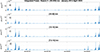 |
Figure 1 The integrated power of electron density fluctuations is measured during the Swarm mission by the Swarm C LP data for four linearly separated frequency bands from December 2013 to April 2023. Panels (a–d) show the integrated power for electron density at scale sizes of (30–450) km, (10–30) km, (10–15) km, and (7.5–10) km, respectively. |
2.3 Loss of navigational capability (LNC) event
The fundamental function of GPS receivers is to provide precise positioning. In order to calculate the navigational equations and obtain accurate positioning information, it is necessary to receive signals from a minimum of four GPS satellites (Spilker Jr et al., 1996). Swarm’s GPS data can help us to define events as a proxy for the disturbed ionosphere. Instances in which receivers lose the ability to track GPS satellites within the receiving antenna’s field of view are known as LOL Xiong et al. (2016); such events serve as a proxy for a disturbed ionosphere. The interrupted signal must reappear within 30 min to qualify as a LOL event. When the interruption lasts more than 30 min, we can assume that the GPS satellite is no longer in the field of view. The observation data files produced by Swarm’s GPS receivers record the number of individual GPS satellite signals received in each epoch. The LNC is defined as an event in which the Swarm GPS receivers can lock on fewer than four GPS satellites. If an LNC event lasts less than a minute, it is considered a single LNC event. However, if the event lasts longer, each minute of loss is considered a unique event, similar to the criteria used for LOL events in Xiong et al. (2016).
Figure 2 shows the electron density profile as a function of magnetic latitude for two incidences of loss of navigational capabilities, including one of the LOL for the Swarm C GPS receiver. On October 29, 2014, two incidences of loss of navigational capabilities occurred in the magnetic conjugate hemispheres. The red scatter plot depicts the number of GPS satellites received by the Swarm C GPS receiver in each epoch. Two black boxes show the electron density profiles for two instances of LNC. In panel (a), the Swarm GPS received signals from less than four satellites in two intervals. Each black box contains a smaller box inside it. These two boxes depict the total LOL events during two LNC occurrences. Inside the first black box, a red box begins at 22:08:12 UT and finishes at 22:08:33 UT. The second black box includes a small green box that spans from 22:14:38 UT to 22:15:02 UT. Panel (b) shows another example of a loss of navigational capabilities on November 1, 2014. This incident has two instances of the total LOL. The first one begins at 23:42:00 UT and ends at 23:43:38 UT, after which one GPS satellite appears for four seconds. Following that, the receiver did not lock onto any GPS satellites from 23:43:38 UT to 23:45:29 UT.
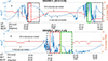 |
Figure 2 Electron density profile for two LNC events. a) The blue line is the electron density profile measured with the Swarm C LP on October 29, 2014. The red broken line shows the number of GPS satellites the Swarm C GPS receivers can lock onto. The black dashed rectangles are electron density profiles during the LNC events. Red and green dashed rectangles are two total LOL events, during which signals from all satellites were disrupted. Panel b) is an LNC event during the November 3, 2014 event. There is just one LNC instance, including two total LOL events. |
2.4 Statistical test for the power-law behavior
We calculate the power-law exponent for sub-intervals of PSD bounded by Xlow and Xhigh using maximum likelihood tests, following the methodology outlined in Baro & Vives (2012). Here, Xlow and Xhigh are lower and higher cutoffs of integrated power, respectively. By adjusting these cutoff values, we can visually depict the estimated values of the exponent γ on a graph using color gradients, creating an exponent map. This map exhibits a triangular pattern due to the rule Xhigh > Xlow. The primary objective of constructing this map is to identify regions with a consistent exponent value. Furthermore, we use the technique described by Yaghoubi et al. (2018) to verify the powerlaw hypothesis for each interval in the map. The p-value is a statistical significance test that can be used to reject the power-law hypothesis at p < 0.1. Our map considers p > 0.1 consistent with a power-law distribution (Yaghoubi et al., 2018). For a dataset including n data points, the likelihood function for a power-law distribution with a specific exponent of γ can be described as:
 (1)
(1)
The probability is denoted as P, and the optimal γ value for the data is the one that maximizes L, which is represented by γmax. Baro & Vives (2012) employed the measure ![Mathematical equation: $ {\left[\frac{{\partial }^2\mathrm{ln}L(\gamma ={\gamma }_{\mathrm{max}})}{{\partial }^2\gamma }\right]}^{-1/2}$](/articles/swsc/full_html/2025/01/swsc240085/swsc240085-eq3.gif) to find the standard deviation of the estimated exponent.
to find the standard deviation of the estimated exponent.
For the goodness of fit, we perform the Kolmogorov-Smirnov (KS) statistical test (Goldstein et al., 2004; Clauset et al., 2009; Yaghoubi et al., 2018; Ghadjari, 2024). This test measures the maximum distance between the empirical and the fitted model’s cumulative distribution functions (CDFs). The p-value test is the probability of observing a KS value larger than the maximum distance between empirical data and the fitted model. For this purpose, we can generate synthetic data with the γ of the fitted model and compare their maximum distance with the fitted model, or alternatively, we can use the theoretical expression used in Yaghoubi et al. (2018) and Deluca & Corral (2013) to measure the p-value:
![Mathematical equation: $$ p\mathbf{Error:02010} \mathrm{value}=2\sum_{\mathrm{i}=1}^{\infty } -{1}^{(i-1)}\mathrm{exp}[-2{i}^2(d\sqrt{n}+0.12d+0.11d/\sqrt[2]{n}], $$](/articles/swsc/full_html/2025/01/swsc240085/swsc240085-eq4.gif) (2)where n is the number of data points in a data set, and d is the maximum distance between CDFs of empirical data and the fitted model. In this study, we use the theoretical expression to measure the p-value.
(2)where n is the number of data points in a data set, and d is the maximum distance between CDFs of empirical data and the fitted model. In this study, we use the theoretical expression to measure the p-value.
2.5 Multifractality test aid intermittency
Multifractal analysis is a tool for demonstrating the intermittent characteristics of turbulence patterns in space plasma physics (Burlaga, 1991; Wawrzaszek & Macek, 2010; Huang et al., 2012; Chian et al., 2022a, b; Gomes et al., 2023). Kantelhardt et al. (2002) addressed two types of multi-fractality in a 1-D signal. Multifractality can be caused by either a broad probability density function, similar to heavy tail distributions, or long-range correlations of fluctuations with values that follow a regular distribution, similar to the Gaussian distribution. The first form of multifractality cannot disappear by rearranging the time series. However, shuffling the time series can reduce or eliminate the second type of multifractality. The multifractal detrended fluctuations analysis (MFDFA) is a method developed by Kantelhardt et al. (2002). This method is widely used in space plasma physics and investigating ionospheric irregularities (Chandrasekhar et al., 2016; Neelakshi et al., 2019, 2022). There are five standard steps in MFDFA. Kantelhardt et al. (2002) contain mathematical detail for each of these steps, and Ihlen (2012) contains the MATLAB implementation of this statistical test.
The first step for a signal with finite length N is converting a noise-like signal to a random-walk signal by the cumulative sum of the signal (Peng et al., 1995; Eke et al., 2000; Hardstone et al., 2012):
 (3)where 〈x〉 is the mean of the signal, and N is the length of signal Xk. The second step is dividing the profile Y(i) into Ns = int(N/s) non-overlapping segments of equal length s. There might be some data points left out of the last segment; then this process needs to be re-done, this time starting from the opposite direction and going backward. Then 2Ns steps are obtained. In the third step, after determining the local trend for each segment, the variance for each segment is calculated:
![Mathematical equation: $$ {F}^2(\nu,s)=1/s\sum_{i=1}^s {\left\{Y[(\nu -1)s+i]-{y}_{\nu }(i)\right\}}^2, $$](/articles/swsc/full_html/2025/01/swsc240085/swsc240085-eq6.gif) (4)for each segment indexed by ν = 1, …, Ns. Also, for the remaining segments, the following must be used:
(4)for each segment indexed by ν = 1, …, Ns. Also, for the remaining segments, the following must be used:
![Mathematical equation: $$ {F}^2(\nu,s)=1/s\sum_{i=1}^s {\left\{Y[(N-(\nu -{N}_s)s+i]-{y}_{\nu }(i)\right\}}^2. $$](/articles/swsc/full_html/2025/01/swsc240085/swsc240085-eq7.gif) (5)
(5)
In (4) and (5)  is a fitting polynomial for the segment ν. The next step is to average the overall segments to obtain the qth-order fluctuation functions
![Mathematical equation: $$ {F}_q(s)\equiv {\left\{1/{N}_s\sum_{\nu =1}^{{N}_s} {\left[{F}^2(\nu,s)\right]}^{q/2}\right\}}^{1/q}, $$](/articles/swsc/full_html/2025/01/swsc240085/swsc240085-eq9.gif) (6)
(6)
Index q in (6) can be any real number. The main goal for multifractal analysis is to find the dependence of q and Fq (s) for different scale sizes of s. Then, we need to repeat steps (4) to (6) for different scale sizes of s. Determining the scaling behavior of the fluctuation functions by analyzing log-log plots Fq (s) versus s for each value q can reveal the multifractal behavior of a signal.
 (7)
(7)
The scaling exponents h(q) are the generalized Hurst exponents, defined by the slope of logFq(s) vs log(s). The second scaling exponent h(2) is the standard Husrt exponent. The Hurst exponent is utilized in numerous studies within space physics and the physics of ionospheric irregularities to assess the presence of persistence, antipersistence, or phase transitions in the system Balasis et al. (2006, 2009); Tanna & Pathak (2014); Lopez-Montes et al. (2015); De Michelis & Tozzi (2020). In the monofractal series, h(q) is independent of q, whereas, in the multifractal series, it depends on q. Whenever q has positive values, h(q) explains the scaling behavior of segments with large fluctuations. Conversely, when q has negative values, it represents the scaling behavior of segments with small fluctuations. The leveling of the generalized Hurst exponent reflects the fact that the q-order Fq is unaffected by the magnitude of the local fluctuations. When the time series has a multifractal structure insensitive to fluctuations of small magnitudes, the multifractal spectrum will have a long left tail. The multifractal spectrum will have a long right tail whenever the time series has a multifractal structure insensitive to local fluctuations with large magnitudes. The generalized Hurst exponent is directly related to the mass exponent t(q) by
 (8)
(8)
The mass exponent  signal for a monofractal has a linear q-dependency and a curved q-dependency for the multifractals.
The last parameter for studying the multifractality of time series with MFDFA is the singularity exponent α and singularity dimension f(α) which are defined by
 (9)
(9)
 (10)
(10)
The plot of a versus f(a) is known as that multifractal spectrum. The multifractal spectrum is a small arc for monofractals, and the value of amax – amin is in the order of 0.1. We used the MATLAB toolbox implemented by Ihlen (2012) to study multifractality and intermittency in the integrated power using several parameters derived based on these steps.
3 Results
Throughout the Swarm’s ten-year mission, we observe 265, 86, and 285 instances of LNC in Swarms A, B, and C, respectively, with a majority of these events occurring in the post-sunset equatorial ionosphere. Among these events, 255, 84, and 268 instances were observed in the postsunset equatorial ionosphere. Recall that Swarm B flew in an orbit between 30–60 km higher than Swarm A and C. The GPS receivers on the Swarm have been upgraded multiple times to improve performance. The last modification to the Swarm C GPS receiver took place on May 6, 2015, while the Swarm A and Swarm B receivers received the last update on October 8, 2015, and October 10, 2015, respectively. From the time of these final updates through 2021, Swarm A and Swarm C experienced three instances of LNC each, whereas Swarm B did not encounter such events until 2022, when solar and geomagnetic activity began to rise significantly.
To explore potential drivers of the intense bursts in integrated power, we qualitatively assess the relationship between solar and geophysical indicators and the corresponding integrated power signals shown in Figure 3, focusing on the temporal alignment of peaks across the different signals. The connection between the F10.7, sunspot numbers (SN), SYM-H, and Ap indices with the third band of integrated power (10–15) km ionospheric structures, is investigated in this work. The 10.7 cm solar radio flux and SN are two solar activity indexes. These two variables are highly correlated. However, F10.7 is a measure of coronal activity, while SN indicates photospheric activity (Zhang et al., 2012). According to Wanliss & Showalter (2006), the SYM-H is a magnetospheric ring current activity marker used to define geomagnetic storms. The Ap index is another geomagnetic index used to represent fluctuations in geomagnetic field activity and indicates storm events (Rostoker, 1972).
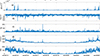 |
Figure 3 Comparison of integrated power with other geomagnetic and solar indices. a) integrated power of electron density fluctuation on a 10–15 km scale during nearly ten years of the Swarm C mission. Panels(b–f) are sym-H, Ap, F10.7, and sunspot number indices, respectively. |
In Figure 3, panel (a) presents the integrated power of plasma density structures with scale sizes between 10–15 km. Panels (b) and (c) show the Sym-H and Ap indices, while panels (d) and (f) display F10.7 and sunspot number (SN), both of which serve as indicators of solar activity. An additional classification based on the Kp index identifies the ten quietest days (Q-days) and five most disturbed days (D-days) of each month. Among the analyzed events, 20 occurred on D-days and 28 on Q-days. A visual inspection of Figure 3 suggests that most geophysical parameters do not show a consistent alignment with the integrated power of density structures, indicating a lack of direct correlation.
In Figure 4, a polar map illustrates the geomagnetic distribution of the LNC events across both hemispheres. The relatively low occurrence of navigational capability loss events between 2015 and 2021 prompts the question of whether the reduced instances of LNC and total LOL occurrences can be attributed to the receiver software updates or the onset of the solar minimum period.
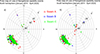 |
Figure 4 Polar map distribution of LNC events during Swarm mission, as a function of magnetic latitude and magnetic local time observed by Swarm satellites between January 2014 and April 2023. Distribution of LNC for a) the north hemisphere, and b) the southern hemisphere. |
We construct a histogram of the strength of density fluctuations measured with the Swarm C for each frequency band of integrated power shown in Figure 5. These histograms exhibit a heavy-tailed distribution. At the largest scale size (first frequency band), the behavior of integrated power differs from the rest of the frequency bands. The histograms of integrated power on the log-log scale for the mesoscale sizes follow a line, indicating a power law. In contrast, the histogram for the largest scale size in log-log space resembles a semi-parabolic curve.
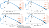 |
Figure 5 Histogram of integrated power in four frequency bands scale size for Swarm-C over nearly ten years. a) Histogram of integrated power for irregularities with scales in the 30–450 km range in the log-log scale. The red circles indicate the number of LNC instances per bin for individual events. The black line represents synthetic data with a normal distribution. Panels (b–d) for integrated power are similar to panel (a) for fluctuations having scale sizes of 15–30 km, 10–15 km, and 7.5–10 km, respectively. |
For the next step of this study, we use the maximum likelihood method to measure the exponents of the PDF for ionospheric structures, which is visualized in panels (b–d) of Figure 5. We also perform a goodness of fit test as described earlier to measure power-law exponents using equation (2) to validate the existence of power-law exponents in the PDFs shown in Figure 5.
Panel (a) of Figure 6 represents the map of the validated exponent, and panel (6b) is the map of plausible p-values for values higher than 0.1. We then filter the data and divide it into smaller groups based on different years and/or magnetic local times periods in the equatorial ionosphere after sunset. Next, the smaller groups are subjected to a similar technique, which generated Figures 5 and 6, leading to comparable results, which indicates that power law PDFs exist even for smaller periods.
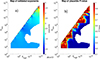 |
Figure 6 Maximum likelihood test to determine the exponents of power law. a) Map of exponents for all possible subintervals that pass goodness of fit test for ionospheric structures with scale sizes of (10–15 km), b) map of subintervals with plausible p-values. |
For the next step, we use the MFDFA, as discussed in Section 2.5 of the study. We utilize the MATLAB package developed by Ihlen (2012). Figure 6 depicts the MFDFA analysis of two years of data taken in the post-sunset equatorial ionosphere in the third band as an illustrative example. The first year is 2014, with the most pronounced fluctuations, and the second year is 2017, with the least significant fluctuations. Panels (7a) and (7d) show generalized Hurst exponents for different orders between −5 < q < 5 for the years 2014 and 2017, respectively. Panels (7b) and (7d) display how mass exponents change for orders between −5 < q < 5 for these two years. Panels (c) and (f) of Figure 6 represent a graph of the multifractal spectrum for the integrated power of electron density fluctuations for the years 2014 and 2017.
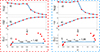 |
Figure 7 Exponents of multifractal detrended fluctuation analysis for the third band of integrated power in 2014 and 2017. a) Generalized q-order Hurst exponents h(q) for q = −5 to q = 5 for density fluctuation power in 2014. b) Mass exponent τ(q) for q orders similar to a). c) The graphical representation of singularity exponent α versus singularity dimension f(α) recognized as the multifractal spectrum. The arrow represents the difference between α’s maximum and minimum. Panels d) to f) are comparable to panels a) to c) for the same integrated power band in 2017. |
4 Statistical analogy between plasma fluctuations and earthquake dynamics
To further interpret the observed power-law behavior in the distribution of integrated power, we introduce a conceptual analogy between ionospheric electron density fluctuations and earthquake dynamics. While we do not claim this analogy as definitive evidence of SOC, we argue that it offers a meaningful statistical framework to interpret rare, high-impact events in the ionosphere. Due to data and satellite orbit limitations, we are unable to directly measure key signatures of selforganized criticality (SOC), such as avalanche duration and spatial scaling. However, several key statistical features – including intermittency, power-law scaling, and heavy-tailed distributions of event magnitude – motivate this comparison.
Figure 8 illustrates four representative ionospheric irregularity examples drawn from the Swarm-C dataset. Each example is shown with its time series of electron density (left column), the corresponding gradient (middle column), and the power spectral density (right column). The gradients reveal rapid, burst-like changes in electron density, resembling the velocity fluctuations seen in seismograms during seismic events. These bursts capture instances of plasma irregularities which, depending on their amplitude, may or may not disrupt GNSS signals. This behavior parallels seismic ground motion, where only sufficiently strong perturbations result in destructive effects, while weaker ones remain undetected or harmless.
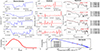 |
Figure 8 Representative ionospheric examples and their statistical characteristics. Each row corresponds to a distinct electron density irregularity example. Column 1: Time series of electron density fluctuations measured by the Swarm-C satellite. Column 2: Corresponding density gradients (ROD). Column 3: Power spectral densities of each event, with fitted slopes around 1.6. Panel E: Histogram of spectral slopes computed from nearly 10 years of data. Panel F: Probability distribution of integrated power of plasma density in the second frequency band, compiled from the 10-year dataset. Colored circles indicate the location of the four representative events. |
The third column of Figure 8 presents power spectra for each ionospheric irregularity example. The spectral slopes are consistently close to 1.6, consistent with the peak of the long-term slope distribution (panel E), and align with expectations from Rayleigh-Taylor-type instabilities widely considered responsible for ionospheric turbulence (Kintner & Seyler, 1985; Nishioka et al., 2011; Bhattacharyya, 2022; Aol et al., 2023; De Michelis et al., 2024). Furthermore, the slope value is slightly less than the expected Kolmogorov scaling value (slope of 5/3 in Kolmogorov, 1991) found in previous works on the power spectra of outflow-driven turbulence (see, for instance, Moraghan et al., 2015, and references therein on star-forming regions). Despite this consistent slope across the four examples, the magnitude of integrated power varies by several orders of magnitude. Panel F highlights this contrast by placing the examples on the integrated power distribution derived from the full 10-year dataset. Although the four examples exhibit nearly identical spectral slopes – suggesting similar underlying turbulence mechanisms – their positions on the power-law distribution differ substantially. Notably, only the example with the highest integrated power (Row D) is an LNC event. This indicates that while spectral slope provides insight into the general instability regime, it does not capture the strength or potential operational impact of an individual event. Integrated power offers a complementary statistical measure that reflects the magnitude of the fluctuation and may serve as a more effective proxy for identifying events likely to result in signal degradation or GNSS loss of lock, such as LNC occurrences. This relationship is analogous to seismology, where different earthquakes may exhibit similar spectral characteristics, but only those with high energy release – reflected in their magnitude – cause significant damage. In both systems, it is not the spectral shape alone but the energy content that determines the severity of the event.
This result highlights the limitations of a turbulence-only perspective: while spectral slopes provide insight into instability mechanisms such as Rayleigh-Taylor turbulence, they do not, on their own, reveal emergent statistical properties of the system. In particular, heavy-tailed distributions, such as those observed in integrated power, are not evident when studying a small number of events in isolation. These emergent features only become visible through ensemble statistics over extended periods. In principle, integrated power values could follow a normal, log-normal, or other distribution, and the presence of a power-law tail is not guaranteed. Just as it is not possible to determine the slope or curvature of a function from only a few points, it is likewise impossible to assess the presence of scale-free behavior without a sufficiently large statistical sample.
The apparent statistical self-similarity of the system is further supported by analyses conducted over shorter temporal windows, as well as by the results of the MFDFA. For instance, when comparing data from the most solar-active year (2014) and a solar-quiet year (2017), the distributions of integrated power in both cases exhibit similar power-law slopes, indicating a persistent scale-invariant structure across different levels of external forcing. However, the distribution from the active year extends to higher magnitudes, consistent with the increased occurrence and intensity of extreme events. The stability of the scaling exponent – despite significant differences in solar activity – reflects a characteristic property of complex systems governed by scale-invariant dynamics. This statistical self-similarity is further corroborated by the similarity of MFDFA parameters between the two years (Figure 7), along with the matching slopes of the corresponding power-law distributions, both of which represent key signatures required for SOC, as discussed in Sornette (2009). Nonetheless, capturing the full dynamic range of event magnitudes – particularly rare, high-power occurrences – requires long-term datasets. The use of a decade-long observation period enables a more comprehensive statistical characterization of the system and strengthens the case for interpreting the observed behavior within a SOC-like framework, supported by heavy-tailed, scale-free distributions.
This observation parallels a central feature of earthquake dynamics: seismic events may share similar spectral content, but their amplitudes – and therefore their consequences – can differ dramatically. In seismology, the Gutenberg-Richter law describes the frequency-magnitude distribution of earthquakes as a power law, where rare, high-magnitude events dominate the tail (Shearer, 2019). Similarly, the distribution of integrated power in ionospheric events exhibits a heavy tail, with rare, large-power events representing potential drivers of critical phenomena such as GNSS loss-of-lock. Within this analogy, the rate of change of density (ROD) plays a role similar to ground velocity in seismograms – while variations are always present, only the largest fluctuations contribute meaningfully to extreme outcomes. Most ROD variations are weak and inconsequential, just as small ground motions are only detectable by sensitive seismometers and do not pose a threat. While it is scientifically valuable to investigate individual strong earthquakes to understand the local conditions that lead to energy release and redistribution within the Earth’s crust, it is equally important to recognize that a statistical perspective reveals emergent behaviors not evident from single events alone.
The same holds for ionospheric electron density irregularities: each event may result from different local drivers such as instability mechanisms, background electron density, or geomagnetic conditions. These individual processes merit separate physical investigations. However, a statistical analysis across a large ensemble of events allows us to uncover scale-invariant features, such as power-law distributions and heavy tails, that hint at deeper organizing principles within the system – features that would remain hidden in an isolated case. This statistical behavior is precisely what motivates our analogy to SOC, where complexity and criticality emerge from the collective dynamics of many interacting events. We emphasize that this remains an analogy, not a direct demonstration. However, the combination of scale-invariant distributions, multifractal intermittency, and rare extreme events with disproportionate impact forms a compelling case for viewing ionospheric turbulence within the same conceptual framework that has been successfully applied to other complex systems, including seismicity.
5 Discussion
It is generally assumed that different regions of the ionosphere are dominated by specific instability mechanisms. For example, in the equatorial zone, the presence of the Rayleigh-Taylor (R-T) instability can be inferred from the slope of the power spectrum of plasma density fluctuations (Kelley et al., 1976; Hudson, 1978; Ott, 1978; Kelley, 2009). In this study, we leverage nearly a decade of precise measurements from the Swarm satellites to investigate the strength of plasma density fluctuations, the Rayleigh-Taylor (R-T) instability in the equatorial ionosphere, and their statistical features. The saturated state observed in the integrated power of electron density is particularly important for space weather studies, as it reveals additional effects that a simple power spectrum cannot capture.
Figure 3 reveals no direct correlation between the integrated power of electron density fluctuations and other geophysical indices shown in this figure which is aligned by Knudsen & Ghadjari (2025). Nevertheless, the overall trend of integrated power aligns with the solar cycle. Several studies have explored the relationship between plasma bubbles and magnetic storms (Stolle et al., 2006; Kumar et al., 2016; Stolle et al., 2024; Huang, 2011a). Huang (2011a) found that bubbles are increased during the main phase of a magnetic storm due to the penetration electric field. Kumar et al. (2016) discovered that the impact of magnetic storms on plasma bubbles is influenced by the local time of storm occurrence. Evening storms enhance the likelihood of plasma bubble formation, while midnight storms suppress irregularity formation in the equatorial ionosphere. These studies, however, did not address the intensity of plasma bubbles.
Figure 4 presents a polar map depicting the spatial distribution of LNC events. These events’ geomagnetic and temporal characteristics align with the observations made by Xiong et al. (2016). Specifically, a higher occurrence of loss of navigational capacity is observed in the northern hemisphere across all three satellites. However, at higher geomagnetic latitudes, the frequency of events is more pronounced in the southern hemisphere. These findings are consistent with the previous study conducted by Xiong et al. (2016), which exclusively reported total LOL in the southern hemisphere at high latitudes. There is a persistent pattern of more LNC events in the southern hemisphere high-latitudes ionosphere during Swarm’s entire mission. In the northern hemisphere, while there have been a few occurrences of loss of navigational capabilities, none have resulted in total lock loss. It is worth noting that there have been no recorded incidents of Swarm B losing navigational capability in the northern hemisphere during the Swarm mission up until April 2023. This satellite operates at an altitude of ~ 510 km, about 80 km higher than the other two spacecraft in the Swarm constellation. The observation that Swarm B experiences approximately one-third the number of LNC events compared to Swarm A and C is consistent with its higher orbital altitude, which corresponds to roughly one atmospheric scale height above the other satellites. This altitude difference reduces the density and intensity of ionospheric irregularities encountered by Swarm B. Our results align with previous studies showing that while electron density fluctuations are present at higher altitudes, their intensity is generally smaller, and the likelihood of forming severe instabilities that disrupt GPS signals decreases Xiong et al. (2016).
Among the LNC events observed during the Swarm mission, 148 out of 267 events observed with Swarm A and 285 events observed with Swarm C, the time separation between events detected with Swarm A and Swarm C, which fly side by side, is less than 150 s. Swarm A and C are separated by only 10 s along-track and 1.4° of longitude cross-track. For 148 events observed on the two satellites within this time period, an irregular region that spans at least 1.4° must be responsible for the LNC events. Furthermore, for 24% of events, LNC is observed twice in one orbit at magnetic conjugate points in opposite hemispheres, which indicates that extreme events happen in conjugate hemispheres for a significant fraction of time. This suggests that the level of turbulence in the conjugate hemispheres is high.
Most LNC events occur in the tail portion of the heavy-tailed probability distribution function shown in Figure 5. This heavy-tailed distribution suggests a physical system capable of generating extreme occurrences. The maximum likelihood and goodness-of-fit tests performed on the third band (5c, 10–15 km) of integrated power, as presented in Figure 6, demonstrate that the distributions shown in Figure 5, panel (c), follow power-law behavior. Similar tests indicate that panels (5b, 15–30 km) and (5d, 7.5–10 km) also follow a power-law behavior. This power-law behavior suggests the presence of SOC within the intensity of the turbulent fluctuations of the ionospheric system. The sampling rate of the Swarm’s Langmuir probe cannot provide sufficient information about power spectrum of the small-scale irregularities, which are crucial for GNSS scintillation. These irregularities are influenced by microinstabilities alongside R-T instability, which limits our ability to infer the physical mechanisms underlying LNC events from the available data.
The power-law behavior observed in the PDF across multiple subintervals, as shown in Figure 5, serves as a robust test to distinguish it from other distributions that can generate extreme events but might resemble a power law either visually or by fitting a line to a whole interval. These findings provide evidence that SOC may statistically describe the turbulence intensity within the equatorial ionosphere, where turbulence dissipates energy through multiscale fluctuations conforming to a power-law probability distribution, as suggested by Smyth et al. (2019) in geophysical turbulence. In contrast to the heavy-tail distributions, systems following normal distributions, such as the Gaussian distribution, are inadequate in explaining the occurrence of high-intensity fluctuations. Therefore, systems that follow a Gaussian behavior do not exhibit extreme phenomena like LNC and LOL events, making them insufficient for modeling ionospheric irregularity fluctuations.
In SOC systems, extreme events do not occur randomly; rather, they emerge as a consequence of the system’s self-organizing dynamics approaching a critical point. These events are primarily driven by intrinsic features and interactions within the system, rather than external physical drivers. One possible interpretation of Figure 5 is that the strength of turbulence structures leading to equatorial plasma bubbles may exhibit characteristics of SOC. Additionally, the statistical features of the system suggest that R-T instability operates across multiple scale sizes to maintain stability. This implies that the internal interactions and dynamics of plasma bubbles play a more significant role in generating extreme events, such as those associated with LNC, compared to the influence of external drivers. This final point is supported by Figure 3, which shows that geomagnetic indices do not align with extreme integrated power in plasma density fluctuations.
The predictability of the likelihood of extreme events in SOC systems holds significant potential for forecasting or nowcasting the occurrence of severe ionospheric irregularities. Additionally, we can deepen our understanding of ionospheric dynamics by comparing ionospheric fluctuations with well-known systems belonging to the same universality classes.
In pure SOC systems, it is implied that the system continuously hovers near an unstable condition. However, in the ionosphere, even in equatorial regions after sunset, irregularities are not always present. According to Balasis et al. (2006), the magnetosphere-ionosphere coupling system experiences intermittent criticality. Therefore, it can be argued that the variation in the intensity of ionospheric irregularities constitutes a critical part of the system, rather than defining the entire ionosphere as a critical system, analogous to how the intensity of avalanches characterizes earthquake dynamics.
The majority of LNC incidents primarily occur in the tail region of the integrated power probability distribution, while only a few occurrences are observed in the low to mid-range integrated power. This indicates that irregularities at the altitude of the Swarm satellites have a higher likelihood of affecting their GPS receivers compared to irregularities above that altitude. If irregularities above the Swarm altitude significantly impacted the Swarm satellites’ GPS receivers, we would expect a higher frequency of LNC incidents in the lower to medium range of integrated power. This finding is consistent with the research by Zakharenkova et al. (2016), which demonstrated a strong correlation between total electron content (TEC) fluctuations and electron density at Swarm altitudes. Furthermore, this observation is supported by comparing the number of LNC incidents between Swarm A and C with Swarm B data, where the number of LNC incidents for Swarm B is less than 30% of the other two satellites.
The integrated power of electron density fluctuations provides a time series of fluctuation strength during the Swarm mission. The results of the MFDFA analysis of the integrated power, shown in Figure 7, reveal that the generalized Hurst exponents for both 2014 and 2017 fall between 0.4 and 1.5. These exponents decrease with q, and the mass exponents for both years deviate from linearity, suggesting the presence of multifractality and intermittency within these signals. The analysis indicates that the integrated power exhibits persistent behavior, as evidenced by h(2) > 0.5. In fractal analysis, persistence means that fluctuations in the system are positively correlated, implying that an increase (or decrease) in values is likely to be followed by further increases (or decreases), reflecting long-term memory or trend continuation in the system (Balasis et al., 2009). This observation aligns with De Michelis et al. (2022), who reported that plasma density fluctuations in the equatorial region predominantly exhibit persistent behavior.
Interestingly, 2014 and 2017 represent two years with distinct solar activity levels, yet the multifractal metrics of the integrated power exhibit similar behavior in both years, indicating that intermittency persists throughout the mission. This suggests that intermittency is a fundamental property of the ionospheric system, not localized to specific regions or conditions. Furthermore, this consistency in multifractal behavior implies that the physical mechanisms driving ionospheric turbulence remain similar across different solar activity phases. During solar maxima, however, the conditions for generating extreme events with higher intensity are more favorable due to the increased potential for higher RODI, which plays a critical role in the formation of stronger instabilities. These findings suggest a self-consistent physical mechanism that operates across different scales and solar conditions, driving the system’s turbulence and intermittency.
The high value of a for both signals shows irregular structures throughout these signals. Our findings align with the research conducted by Neelakshi et al. (2022), which performed MFDFA analysis on in-situ electron density obtained through a rocket experiment to explore the scale features of electron density fluctuations in the E-F valley of the equatorial ionosphere. However, it is important to indicate that their research utilized in-situ plasma density data directly, whereas we generated the integrated power from in-situ electron density observations. Referring to Figure 11 of Ihlen (2012), a long left tail in the h(q) function indicates a multifractal structure that remains unaffected by small-magnitude fluctuations. In this analysis, the type of multifractality observed for the strength of the ionospheric turbulence fluctuations is not sensitive to shuffling due to the power-law PDF distribution exhibited by the fluctuations.
The presence of turbulence intermittency, as demonstrated through MFDFA analysis, along with the occurrence of strong bursts at the tail of the integrated power probability density function of electron density fluctuations, provides additional support for the findings presented by De Michelis et al. (2021b), and De Michelis et al. (2022). These studies underline the importance of intermittency and high RODI levels as critical characteristics in events involving the loss of GPS signal lock. The correlation between our data and the studies mentioned above underscores the significance of intermittency and elevated RODI levels in comprehending and predicting lock loss events in the ionosphere.
The integrated power represents the strength of fluctuations in specific density structures. We show that intermittency in ionospheric irregularity fluctuations is not confined to small scales but can occur across all scales we studied, from the smallest scale in the order of kilometers to hundreds of kilometers. This finding agrees with McComb & May (2018) and the new definitions of turbulence intermittency, indicating that intermittency can be relevant at different scales.
Turbulence intermittency has been extensively studied through various mechanisms, particularly in the context of passive scalar transport in turbulent media (Kraichnan, 1994; Shraiman & Siggia, 2000; Warhaft, 2000; Falkovich et al., 2001). These works highlight how intermittent and multiscale structures in turbulence emerge from chaotic advection, energy cascades, and anomalous diffusion processes. Specifically, Kraichnan (1994) and Falkovich et al. (2001) emphasize the role of multifractal behavior in passive scalar transport, demonstrating that turbulence structures at different scales exhibit varying degrees of scaling anomalies. Shraiman & Siggia (2000) and Warhaft (2000) further show that the mixing of passive scalars in turbulent flows leads to intermittent structures, but the underlying physical mechanisms differ from those in SOC, where local instability and threshold-driven events dictate behavior.
While this study confirms that intermittency also exists in the equatorial region, Consolini et al., 2020 highlights that it is a prominent feature of high latitudes, where the ionosphere is directly influenced by geomagnetic storms and substorms. In contrast, the equatorial ionosphere is comparatively isolated from such disturbances, as illustrated in Figure 3. Additionally, Figure 5 demonstrates that when each spatial scale is analyzed separately, turbulence intensity follows a power-law distribution. This is distinct from the broader concept of turbulence spanning multiple spatial scales, where interactions between different scale sizes play a crucial role. Instead, our findings suggest that the statistical behavior of each individual scale exhibits a well-defined power-law structure.
Rather than treating turbulence intermittency and SOC as mutually exclusive descriptions, newer studies suggest that SOC provides an additional statistical perspective on how energy dissipates in large-scale systems. While turbulence describes the general mechanism of energy transfer across scales, SOC explains the size distribution of avalanches – energy release events that can span multiple orders of magnitude but still follow a power-law distribution. This behavior is analogous to earthquake dynamics, where the distribution of event sizes follows a power law, distinguishing it from systems that simply exhibit multiscale structures without power-law behavior.
Furthermore, prior studies have demonstrated that intermittency and SOC can coexist in complex dynamical systems. Uritsky et al. (2007) and Klimas et al. (2007) have shown that intermittent turbulence and SOC-like avalanche dynamics emerge together in space plasma environments, challenging the traditional notion that these processes operate independently. This reinforces the idea that while the ionosphere follows a multiscale cascade, the power-law behavior observed at distinct scales could be linked to SOC-like processes governing energy release and structural reorganization. Future research should explore the extent to which SOC-like mechanisms influence the evolution of ionospheric turbulence, particularly in the context of energy dissipation and self-organization across different latitudinal regions.
While power-law distributions are often cited as evidence for SOC, Boffetta et al. (1999) demonstrated that turbulence in solar flares can also produce power-law statistics, challenging the idea that such behavior uniquely indicates SOC. Their analysis of waiting time distributions found that the power-law scaling was more consistent with turbulence rather than a SOC avalanche model, emphasizing the need for additional criteria beyond power-law behavior alone. While Boffetta et al. (1999) analyzed power-law scaling in segmented waiting time distributions, our approach systematically investigates power-law behavior across multiple subintervals, generating a robustness map that validates the power-law hypothesis at different scales. Furthermore, our study focuses on the intensities of plasma density irregularities, which emerge from turbulence and are more directly analogous to avalanches in SOC models, whereas Boffetta et al. (1999) primarily examined waiting times between events. This ensures that the observed power-law scaling is not an artifact of selection bias or arbitrary cut-offs, providing a more rigorous test for SOC in ionospheric turbulence.
This study represents the first attempt to investigate self-organized SOC as a statistical feature of the strength of fluctuations in the equatorial ionosphere. The probability density function (PDF) of the integrated power suggests that these fluctuations follow a power-law behavior indicative of SOC. However, due to the limitations imposed by the sampling frequency of the Langmuir probe, our analysis is restricted to kilometer-scale irregularities, precluding the study of smaller-scale fluctuations. Additionally, the moving platform of the satellite prevents us from analyzing the temporal evolution of ionospheric irregularities, which is critical for a comprehensive assessment of SOC. To enable more robust analyses of SOC and ionospheric turbulence, it is necessary to design dedicated missions specifically to study ionospheric irregularities or to develop advanced theoretical models. Moreover, the complex dynamics of the ionosphere, spanning various spatial and temporal scales, present additional challenges. While SOC provides a statistical framework for understanding the strength of turbulence fluctuations across scales, it is important to note that this interpretation complements, rather than replaces, the dynamic and multifaceted nature of ionospheric turbulence.
6 Conclusions
The majority of LNC events coincide with the tail of a power-law PDF for plasma structures across multiple spatial scales (7.5–30 km). The power-law behavior, confirmed by maximum likelihood and goodness-of-fit tests, suggests the presence of potential SOC in ionospheric turbulence. The scale-free nature of SOC implies that events of varying magnitudes, including extreme events like LNC, are intrinsic to the system’s internal dynamics.
GPS receivers on Swarm A and C, orbiting at altitudes between 430–460 km, suffer more frequent lLNC than on Swarm B (at 530 km). The reappearance of LNC events after 2021, coinciding with increased solar activity, further underscores the influence of solar phenomena on ionospheric irregularities and their disruptive effects on GNSS.
MFDFA reveals the multifractal and intermittent nature of the fluctuations across all frequency bands, indicating that intermittency is not limited to small-scale structures. The findings emphasize the importance of considering intermittency and large-scale fluctuations in understanding and predicting the impact of ionospheric irregularities on GNSS.
The evidence for potential SOC in ionospheric turbulence opens new avenues for research. By exploring the predictability of extreme events and leveraging the concept of universality classes, we can gain deeper insights into the underlying mechanisms of ionospheric irregularities and potentially improve forecasting and mitigation strategies for GNSS disruptions. Future studies should focus on establishing a more robust connection between SOC and ionospheric dynamics, and investigate the potential for predicting extreme space weather events based on SOC principles.
Acknowledgments
We thank Vadim M. Uritsky, Giuseppe Consolini, Ryan McGranaghan, Mohammad Hasan Yaghoubi, Omid Khajehdehi, Hersh Gilbert, and Reihaneh Ghaffari for their helpful discussions. The editor thanks two anonymous reviewers for their assistance in evaluating this paper.
Funding
Swarm is a European Space Agency mission. This study is undertaken with the financial support of the Canadian Space Agency (15SUSWARM), the Natural Sciences and Engineering Research Council of Canada, and the European Space Agency. Georgios Balasis’s work has been supported as part of Swarm DISC (Data, Innovation, and Science Cluster) activities funded by ESA contract number: 4000109587.
Data availability statement
Hourly-averaged solar wind and geomagnetic indices were obtained from the OMNIWeb database (https://omniweb.gsfc.nasa.gov/form/dx1.html). The classification of the ten quietest days (Q-days) and five most disturbed days (D-days) per month was based on Kp index data provided by the GFZ Potsdam repository (http://www.gfz-potsdam.de/en/section/earths-magnetic-field/data-products-services/kp-index/qd-days).
Swarm mission data, including Langmuir probe measurements and RINEX files, are available from the ESA Swarm Data, Innovation, and Science Cluster (Swarm DISC) at https://swarm-diss.eo.esa.int.
References
- Aol, S, Buchert S, Jurua E, Sorriso-Valvo L. 2023. Spectral properties of sub-kilometer-scale equatorial irregularities as seen by the Swarm satellites. Adv Space Res 72 (3): 741–752. https://doi.org/10.1016/j.asr.2022.07.059. [Google Scholar]
- Bak, P, Chen K, Tang C. 1990. A forest-fire model and some thoughts on turbulence. Phys Lett A 147 (5–6): 297–300. https://doi.org/10.1016/0375-9601(90)90451-S. [Google Scholar]
- Bak, P, Tang C, Wiesenfeld K. 1987. Self-organized criticality: An explanation of the 1/f noise. Phys Rev Lett 59 (4): 381. https://doi.org/10.1103/PhysRevA.38.364. [Google Scholar]
- Balasis, G, Balikhin MA, Chapman SC, Consolini G, Daglis IA, et al. 2023a. Complex systems methods characterizing nonlinear processes in the near-earth electromagnetic environment: Recent advances and open challenges. Space Sci Rev 219 (5): 38. https://doi.org/10.1007/s11214-023-00979-7. [Google Scholar]
- Balasis, G, Boutsi AZ, Papadimitriou C, Potirakis SM, Pitsis V, Daglis IA, Anastasiadis A, Giannakis O. 2023b. Investigation of dynamical complexity in Swarm-derived geomagnetic activity indices using information theory. Atmosphere 14 (5): 890. https://doi.org/10.3390/atmos14050890. [Google Scholar]
- Balasis, G, Daglis I, Kapiris P, Mandea M, Vassiliadis D, Eftaxias K. 2006. From pre-storm activity to magnetic storms: a transition described in terms of fractal dynamics. Ann Geophys 24: 3557–3567. Copernicus Publications Gottingen, Germany. https://doi.org/10.5194/angeo-24-3557-2006. [Google Scholar]
- Balasis, G, Daglis IA, Anastasiadis A, Papadimitriou C, Mandea M, Eftaxias K. 2011a. Universality in solar flare, magnetic storm and earthquake dynamics using Tsallis statistical mechanics. Physica A Stat Mech Appl 390 (2): 341–346. https://doi.org/10.1016/j.physa.2010.09.029. [Google Scholar]
- Balasis, G, Daglis IA, Papadimitriou C, Kalimeri M, Anastasiadis A, Eftaxias K. 2009. Investigating dynamical complexity in the magnetosphere using various entropy measures. J Geophys Res Space Phys 114 (A9). https://doi.org/10.3390/atmos14050890. [Google Scholar]
- Balasis, G, Papadimitriou C, Daglis I, Anastasiadis A, Sandberg I, Eftaxias K. 2011b. Similarities between extreme events in the solar-terrestrial system by means of nonextensivity. Nonlinear Process Geophys 18 (5): 563–572. https://doi.org/10.5194/npg-18-563-2011. [Google Scholar]
- Barabasi, A-L. 2005. The origin of bursts and heavy tails in human dynamics. Nature 435 (7039): 207–211. https://doi.org/10.1038/nature03459. [Google Scholar]
- Baro, J, Vives E. 2012. Analysis of power-law exponents by maximum-likelihood maps. Phys Rev E 85 (6): 066121. https://doi.org/10.1103/PhysRevE.85.066121. [Google Scholar]
- Batchelor, GK, Townsend AA. 1949. The nature of turbulent motion at large wave-numbers. Proc R Soc Lond A Math Phys Sci 199 (1057): 238–255. https://doi.org/10.1098/rspa.1949.0136. [Google Scholar]
- Beggs, JM, Plenz D. 2003. Neuronal avalanches in neocortical circuits. J Neurosci 23 (35): 11167–11177. https://doi.org/10.1523/JNEUROSCI.23-35-11167.2003. [Google Scholar]
- Bhattacharyya, A. 2022. Equatorial plasma bubbles: A review. Atmosphere 13 (10): 1637. https://doi.org/10.3390/at-mos13101637. [CrossRef] [Google Scholar]
- Bishop, G, Klobuchar J, Basu S, Clynch J, Coco D. 1990. Measurements of Trans-Ionospheric Effects Using Signals from GPS. Tech. Rep. Geophysics Lab (AFSC), Hanscom AFB, MA. https://apps.dtic.mil/sti/html/tr/ADP006316/index.html. [Google Scholar]
- Boffetta, G, Carbone V, Giuliani P, Veltri P, Vulpiani A. 1999. Power laws in solar flares: self-organized criticality or turbulence? Phys Rev Lett 83 (22): 4662. https://doi.org/10.1103/PhysRevLett.83.4662. [Google Scholar]
- Bryson, MC. 1974. Heavy-tailed distributions: properties and tests. Technometrics 16 (1): 61–68. https://doi.org/10.1080/00401706.1974.10489150. [CrossRef] [MathSciNet] [Google Scholar]
- Burlaga, L. 1991. Intermittent turbulence in the solar wind. J Geophys Res Space Phys 96 (A4): 5847–5851. https://doi.org/10.1029/91JA00087. [Google Scholar]
- Calif, R, Schmitt FG, Huang Y, Soubdhan T. 2013. Intermittency study of high frequency global solar radiation sequences under a tropical climate. Sol Energy 98: 349–365. https://doi.org/10.1016/j.solener.2013.09.018. [Google Scholar]
- Chandrasekhar, E, Prabhudesai SS, Seemala GK, Shenvi N. 2016. Multifractal detrended fluctuation analysis of ionospheric total electron content data during solar minimum and maximum. J Atmos Sol-Terr Phys 149: 31–39. https://doi.org/10.1016/j.jastp.2016.09.007. [Google Scholar]
- Chang, T. 1999. Self-organized criticality, Multi-fractal spectra, Sporadic localized reconnections and Intermittent turbulence in the magnetotail. Phys Plasmas 6 (11): 4137–4145. https://doi.org/10.1063/1.873678. [Google Scholar]
- Chang, T, Tam SW, Wu C-C. 2004. Complexity induced anisotropic bimodal intermittent turbulence in space plasmas. Phys Plasmas 11 (4): 1287–1299. https://doi.org/10.1063/1.1667496. [Google Scholar]
- Chang, T, Wu C, Podesta J, Echim M, Lamy H, Tam S. 2010. ROMA (Rank-Ordered Multifractal Analyses) of intermittency in space plasmas-a brief tutorial review. Nonlin Processes Geophys 17 (5): 545–551. https://doi.org/10.5194/npg-17-545-2010. [Google Scholar]
- Chian, AC-L, Abalde JR, Miranda RA, Borotto FA, Hysell DL, Rempel EL, Ruffolo D. 2018. Multi-spectral optical imaging of the spatiotemporal dynamics of ionospheric intermittent turbulence. Sci Rep 8 (1): 1–15. https://doi.org/10.1038/s41598-018-28780. [CrossRef] [Google Scholar]
- Chian, AC-L, Borotto F, Hada T, Miranda RA, Muñoz PR, Rempel EL. 2022a. Chaos, complexity, and intermittent turbulence in space plasmas. arXiv preprint arXiv:2204.06133. https://doi.org/10.48550/arXiv.2204.06133. [Google Scholar]
- Chian, AC-L, Borotto FA, Hada T, Miranda R, Muñoz P, Rempel E. 2022b. Nonlinear dynamics in space plasma turbulence: temporal stochastic chaos. Rev Mod Plasma Phys 6 (1): 1–56. https://doi.org/10.1007/s41614-022-00095-z. [Google Scholar]
- Clauset, A. 2018. Trends and fluctuations in the severity of interstate wars. Sci Adv 4 (2): eaao3580. https://doi.org/10.1126/sciadv.aao3580. [Google Scholar]
- Clauset, A, Shalizi CR, Newman ME. 2009. Power-law distributions in empirical data. SIAM Rev 51 (4): 661–703. https://doi.org/10.1126/sciadv.aao3580. [CrossRef] [Google Scholar]
- Consolini, G, and Chang T. 2002. Complexity, magnetic field topology, criticality, and metastability in magnetotail dynamics. J Atmos Sol-Terr Phys 64 (5–6): 541–549. https://doi.org/10.1016/S1364-6826(02)00011-1. [Google Scholar]
- Consolini, G, De Michelis P, Alberti T, Coco I, Giannattasio F, Tozzi R, Carbone V. 2020. Intermittency and passive scalar nature of electron density fluctuations in the high-latitude ionosphere at Swarm Altitude. Geophy Res Lett 47 (18): e2020GL089628. https://doi.org/10.1029/2020GL089628. [Google Scholar]
- Cooke, R, Nieboer D. 2011. Heavy-tailed distributions: Data, diagnostics, and new developments. Resources for the Future Discussion Paper 9: 11–19. https://papers.ssrn.com/sol3/papers.cfm?abstract_id=1811043. [Google Scholar]
- Costa, E, Kelley M. 1977. Ionospheric scintillation calculations based on in situ irregularity spectra. Radio Sci 12 (5): 797–809. https://doi.org/10.1029/RS012i005p00797. [CrossRef] [Google Scholar]
- De Michelis, P, Consolini G, Alberti T, Pignalberi A, Coco I, Tozzi R, Giannattasio F, Pezzopane M. 2024. Investigating Equatorial Plasma Depletions through CSES-01 Satellite Data. Atmosphere 15 (7): 868. https://doi.org/10.3390/atmos15070868. [Google Scholar]
- De Michelis, P, Consolini G, Pignalberi A, Lovati G, Pezzopane M, Tozzi R, Giannattasio F, Coco I, Marcucci MF. 2022. Ionospheric turbulence: A challenge for GPS loss of lock understanding. Space Weather 20 (7): e2022SW003129. https://doi.org/10.1029/2022SW003129. [Google Scholar]
- De Michelis, P, Consolini G, Pignalberi A, Tozzi R, Coco I, Giannattasio F, Pezzopane M, Balasis G. 2021a. Looking for a proxy of the ionospheric turbulence with Swarm data. Sci Rep 11 (1): 6183. https://doi.org/10.1038/s41598-021-84985-1. [Google Scholar]
- De Michelis, P, Consolini G, Tozzi R, Pignalberi A, Pezzopane M, Coco I, Giannattasio F, Marcucci MF. 2021b. Ionospheric turbulence and the equatorial plasma density irregularities: Scaling features and RODI. Rem Sens 13 (4): 759. https://doi.org/10.3390/rs13040759. [Google Scholar]
- De Michelis, P, Tozzi R. 2020. Multiscale analysis of the turbulent ionospheric medium. In: The Dynamical Ionosphere, Elsevier, pp. 301–312. ISBN: 978-0-12-814782-5. https://doi.org/10.1016/B978-0-12-814782-5.00019-4. [Google Scholar]
- Deluca, A, Corral JA. 2013. Fitting and goodness-of-fit test of non-truncated and truncated power-law distributions. Acta Geophys 61: 1351–1394. https://doi.org/10.2478/s11600-013-0154-9. [Google Scholar]
- Dennis, BR. 1988. Solar flare hard X-ray observations. Sol Phys 118: 49–94. https://doi.org/10.1007/BF00148588. [Google Scholar]
- Di Mare, F, Spicher A, Clausen LBN, Miloch WJ, Moen JI. 2021. Turbulence and Intermittency in the Winter Cusp Ionosphere Studied With the ICI Sounding Rockets. J Geophys Res Space Phys 126 (8): e2021JA029150. https://doi.org/10.1029/2021JA029150. [CrossRef] [Google Scholar]
- Dragulescu, A, Yakovenko VM. 2000. Statistical mechanics of money. Eur Phys J B Condens Matter Complex Syst 17: 723–729. https://doi.org/10.1007/s100510070114.pdf. [Google Scholar]
- Dudok de Wit, T, Krasnosel’skikh V. 1996. Non-Gaussian statistics in space plasma turbulence: fractal properties and pitfalls. Nonlin Processes Geophys 3 (4): 262–273. https://doi.org/10.5194/npg-3-262-1996. [Google Scholar]
- Dyrud, L, Krane B, Oppenheim M, Pecseli H, Trulsen J, Wernik A. 2008. Structure functions and intermittency in ionospheric plasma turbulence. Nonlin Processes Geophys 15 (6): 847–862. https://doi.org/10.5194/npg-15-847-2008. [CrossRef] [Google Scholar]
- Eke, A, Herman P, Bassingthwaighte J, Raymond G, Percival D, Cannon M, Balla I, Ikrenyi C. 2000. Physiological time series: distinguishing fractal noises from motions. Pflugers Archiv 439: 403–415. https://doi.org/10.1007/s004249900135. [Google Scholar]
- Fæhn Follestad, A, Herlingshaw K, Ghadjari H, Knudsen DJ, McWilliams KA, Moen JI, Spicher A, Wu J, Oksavik K. 2020. Dayside field-aligned current impacts on ionospheric irregularities. Geophys Res Lett 47 (11): e2019GL086722. https://doi.org/10.1029/2019GL086722. [Google Scholar]
- Falkovich, G, Gawdzki K, Vergassola M. 2001. Particles and fields in fluid turbulence. Rev Mod Phys 73 (4): 913. https://doi.org/10.1103/RevModPhys.73.913. [Google Scholar]
- Farge, M. 1992. Wavelet transforms and their applications to turbulence. Ann Rev Fluid Mech 24 (1): 395–458. https://doi.org/10.1146/annurev.fl.24.010192.002143. [Google Scholar]
- Friis-Christensen, E, Luhr H, Hulot G. 2006. Swarm: A constellation to study the Earth’s magnetic field. Earth Planet Space 58, 351–358. https://doi.org/10.1016/j.asr.2006.10.008. [CrossRef] [Google Scholar]
- Frisch, U. 1980. Fully developed turbulence and intermittency. Ann New York Acad Sci 357: 359–367. https://doi.org/10.1111/j.1749-6632.1980.tb29703.x. [Google Scholar]
- Garber, A, Hallerberg S, Kantz H. 2009. Predicting extreme avalanches in self-organized critical sandpiles. Phys Rev E 80 (2): 026124. https://doi.org/10.1103/PhysRevE.80.026124. [Google Scholar]
- Ghadjari, H. 2024. Swarm-Based study of the disturbed and quiet equatorial ionosphere. PhD Thesis, University of Calgary. https://prism.ucalgary.ca/bitstreams/b37fa952-8c14-4e2d-b094-9a1b365394ee/download. [Google Scholar]
- Ghadjari, H, Knudsen D, Skone S. 2022. Standing Alfven waves within equatorial plasma bubbles. Geophys Res Lett 49 (7): e2021GL097526. https://doi.org/10.1029/2021GL097526. [CrossRef] [Google Scholar]
- Ghadjari, H, Knudsen D, Skone S. 2023. Probability distribution of integrated power of equatorial ionosphere plasma density fluctuations measured by the Swarm Langmuir probes. In: EGU General Assembly Conference Abstracts, EGU-8677. https://doi.org/10.5194/egusphere-egu23-8677. [Google Scholar]
- Ghaffari, R. 2022. Characterizing energetic electron precipitation and whistler-mode waves during electron injection events. Ca876061-d396-4122-b3b4-c247c439d124. http://hdl.handle.net/1880/114284. [Google Scholar]
- Ghaffari, R, Cully CM. 2020. Statistical study of whistler-mode waves during substorm injections. AGU Fall Meeting Abstracts 2020: SM009-12. [Google Scholar]
- Ghaffari, R, Cully CM, Gabrielse C. 2021. Statistical study of whistler-mode waves and expected pitch angle diffusion rates during dispersionless electron injections. Geophy Res Lett 48 (17): e2021GL094085. https://doi.org/10.1029/2021GL094085. [Google Scholar]
- Giannattasio, F, De Michelis P, Consolini G, Quattrociocchi V, Coco I, Tozzi R. 2019. Characterising the electron density fluctuations in the high-latitude ionosphere at Swarm altitude in response to the geomagnetic activity. Ann Geophys 62(4): GM453. https://doi.org/10.4401/ag-7790. [Google Scholar]
- Goldstein, ML, Morris SA, Yen GG. 2004. Problems with fitting to the power-law distribution. Eur Phys J B Condens Matter Complex Syst 41: 255–258. https://doi.org/10.1140/epjb/e2004-00316-5. [Google Scholar]
- Gomes, LF, Gomes TF, Rempel EL, Gama S. 2023. Origin of multifractality in solar wind turbulence: the role of current sheets. Mon Not R Astron Soc 519 (3): 3623–3634. https://doi.org/10.1093/mnras/stac3577. [Google Scholar]
- Hajj, MR. 1999. Intermittency of energy-containing scales in atmospheric surface layer. J Eng Mech 125 (7): 797–803. https://doi.org/10.1061/(ASCE)0733-9399(1999)125:7(797). [Google Scholar]
- Hamza, AM, Song K, Meziane K, Thayyil JP. 2023. Two-component phase scintillation spectra in the auroral region: Observations and Model. J Geophys Res Space Phys 129 (1): e2023JA031998. https://doi.org/10.1029/2023JA031998. [Google Scholar]
- Hardstone, R, Poil S-S, Schiavone G, Jansen R, Nikulin VV, Mansvelder HD, Linkenkaer-Hansen K. 2012. Detrended fluctuation analysis: a scale-free view on neuronal oscillations. Front Physiol 3: 450. https://doi.org/10.3389/fphys.2012.00450/full. [Google Scholar]
- Huang, C. 2011. Occurrence of equatorial plasma bubbles during intense magnetic storms. Int J Geophys 54 (3): 435–442. https://doi.org/10.1155/2011/401858. [Google Scholar]
- Huang, S, Zhou M, Sahraoui F, Vaivads A, Deng X, et al., 2012. Observations of turbulence within reconnection jet in the presence of guide field. Geophy Res Lett 39 (11): L11104. https://doi.org/10.1029/2012GL052210. [Google Scholar]
- Hudson, MK. 1978. Spread F bubbles: Nonlinear Rayleigh-Taylor mode in two dimensions. J Geophys Res Space Phys 83 (A7): 3189–3194. https://doi.org/10.1029/JA083iA07p03189. [Google Scholar]
- Hussain, AF. 1986. Coherent structures and turbulence. J Fluid Mech 173: 303–356. https://doi.org/10.1017/S0022112086001192. [Google Scholar]
- Ihlen, EA. 2012. Introduction to multifractal detrended fluctuation analysis in Matlab. Front Physiol 3: 141. https://doi.org/10.3389/fphys.2012.00141. [Google Scholar]
- Iliopoulos, AC, Pavlos GP, Papadimitriou E, Sfiris DS, Athanasiou M, Tsoutsouras V. 2012. Chaos, self organized criticality, intermittent turbulence and nonextensivity revealed from seismogenesis in north Aegean area. Int J Bifurc Chaos 22 (09): 1250224. https://doi.org/10.1142/S0218127412502240. [Google Scholar]
- Ivanov, PC, Amaral LAN, Goldberger AL, Havlin S, Rosenblum MG, Struzik ZR, Stanley HE. 1999. Multifractality in human heartbeat dynamics. Nature 399 (6735): 461–465. https://doi.org/10.1038/20924. [Google Scholar]
- Jayachandran, P, Hamza A, Hosokawa K, Mezaoui H, Shiokawa K. 2017. GPS amplitude and phase scintillation associated with polar cap auroral forms. J Atmos Sol-Terr Phys 164: 185–191. https://doi.org/10.1016/j.jastp.2017.08.030. [CrossRef] [Google Scholar]
- Jin, Y, Moen JI, Spicher A, Oksavik K, Miloch WJ, Clausen LB, Pozoga M, Saito Y. 2019. Simultaneous rocket and scintillation observations of plasma irregularities associated with a reversed flow event in the cusp ionosphere. J Geophys Res Space Phys 124 (8): 7098–7111. https://doi.org/10.1029/2019JA026942. [Google Scholar]
- Kadanoff, LP, Nagel SR, Wu L, Zhou S-M. 1989. Scaling and universality in avalanches. Phys Rev A 39 (12): 6524. https://doi.org/10.1103/PhysRevA.39.6524. [Google Scholar]
- Kantelhardt, JW, Zschiegner SA, Koscielny-Bunde E, Havlin S, Bunde A, Stanley HE. 2002. Multifractal detrended fluctuation analysis of nonstationary time series. Phys A Stat Mech Appl 316 (1–4): 87–114. https://doi.org/10.1016/S0378-4371(02)01383-3. [Google Scholar]
- Kelley MC. 2009. The Earth’s ionosphere: Plasma physics and electrodynamics. Int Geophys 96: xiii–xiv. Academic Press. https://doi.org/10.1016/B978-0-12-404013-7.X5001-1. [Google Scholar]
- Kelley, MC, Haerendel G, Kappler H, Valenzuela A, Balsley B, Carter DA, Ecklund WL, Carlson C, Hausler B, Torbert R. 1976. Evidence for a Rayleigh-Taylor type instability and upwelling of depleted density regions during equatorial spread F. Geophy Res Lett 3 (8): 448–450. https://doi.org/10.1029/GL003i008p00448. [Google Scholar]
- Keskinen, M, Ossakow S, Basu S, Sultan P. 1998. Magnetic-flux-tube-integrated evolution of equatorial ionospheric plasma bubbles. J Geophys Res Space Phys 103 (A3): 3957–3967. https://doi.org/10.1029/97JA02192. [Google Scholar]
- Kil, H. 2015. The morphology of equatorial plasma bubbles-a review. J Astron Space Sci 32 (1): 13–19. https://doi.org/10.5140/JASS.2015.32.1.1. [Google Scholar]
- Kil, H, Heelis RA, Paxton LJ, Oh S-J. 2009. Formation of a plasma depletion shell in the equatorial ionosphere. J Geophys Res Space Phys 114 (A11): A11302. https://doi.org/10.1029/2009JA014369. [Google Scholar]
- Kintner, PM, CE Seyler. 1985. The status of observations and theory of high latitude ionospheric and magnetospheric plasma turbulence. Space Sci Rev 41 (1–2): 91–129. https://doi.org/10.1007/BF00241347. [CrossRef] [Google Scholar]
- Kivanç, Ö, Heelis RA. 1998. Spatial distribution of ionospheric plasma and field structures in the high-latitude F region. J Geophys Res Space Phys 103 (A4): 6955–6968. https://doi.org/10.1029/97JA03237. [Google Scholar]
- Klimas, AJ, Uritsky VM, Paczuski M. 2007. Self-organized criticality and intermittent turbulence in an MHD current sheet with a threshold instability. arXiv preprint astro-ph/0701486. https://doi.org/10.48550/arXiv.astro-ph/0701486. [Google Scholar]
- Klobuchar, JA. 1983. Ionospheric effects on Earth-space propagation. Tech. Rep. Air Force Geophysics Lab, Hanscom AFB, MA, 19850020921. [Google Scholar]
- Knudsen, D, Burchill J, Buchert S, Eriksson A, Gill R, Wahlund J-E, Ahlen L, Smith M, Moffat B. 2017. Thermal ion imagers and Langmuir probes in the Swarm electric field instruments. J Geophys Res Space Phys 122 (2): 2655–2673. https://doi.org/10.1002/2016JA022571. [CrossRef] [Google Scholar]
- Knudsen, D, Ghadjari H. 2025. Investigating the role of geomagnetic activity in loss of navigational capability in the Swarm Satellite Mission. In: EGU General Assembly 2025, Vienna, Austria. https://doi.org/10.5194/egusphere-egu25-14321. [Google Scholar]
- Kolmogorov, AN. 1991. The local structure of turbulence in incompressible viscous fluid for very large Reynolds numbers. Proc R Soc Lond A Math Phys Sci 434 (1890): 9–13. https://doi.org/10.1098/rspa.1991.0075. [Google Scholar]
- Kraichnan, RH. 1994. Anomalous scaling of a randomly advected passive scalar. Phys Rev Lett 72 (7): 1016. https://doi.org/10.1103/PhysRevLett.72.1016. [Google Scholar]
- Kumar, S, Chen W, Liu Z, Ji S. 2016. Effects of solar and geomagnetic activity on the occurrence of equatorial plasma bubbles over Hong Kong. J Geophys Res Space Phys 121 (9): 9164–9178. https://doi.org/10.1002/2016JA022873. [CrossRef] [Google Scholar]
- Li, R, Lei J. 2021. The determination of satellite orbital decay from POD data during geomagnetic storms. Space Weather 19 (4): e2020SW002664. https://doi.org/10.1029/2020SW002664. [Google Scholar]
- Lopez-Montes, R, Perez-Enriquez R, Araujo-Pradere EA, Cruz-Abeyro JAL. 2015. Fractal and wavelet analysis evaluation of the mid latitude ionospheric disturbances associated with major geomagnetic storms. Adv Space Res 55 (2): 586–596. https://doi.org/10.1016/j.asr.2014.10.037. [Google Scholar]
- Lovejoy, S, Schertzer D. 1991. Multifractal analysis techniques and the rain and cloud fields from 10- 3 to 10 6 m. In: Non-Linear Variability in Geophysics: Scaling and Fractals , Schertzer D, Lovejoy S (Eds.), Springer Netherlands, Dordrecht, pp.111–144. ISBN: 978-94-009-2147-4. https://doi.org/10.1007/978-94-009-2147-4_8. [Google Scholar]
- Lu, ET, Hamilton RJ. 1991. Avalanches and the distribution of solar flares. Astrophys J 380: L89–L92. https://doi.org/10.1086/186180. [Google Scholar]
- Lui, A. 2002. Multiscale phenomena in the near-Earth magnetosphere. J Atmos Sol-Terr Phys 64 (2): 125–143. https://doi.org/10.1016/S1364-6826(01)00079-7. [Google Scholar]
- Lux, T, Marchesi M. 1999. Scaling and criticality in a stochastic multi-agent model of a financial market. Nature 397 (6719): 498–500. https://doi.org/10.1038/17290. [Google Scholar]
- McClure, J, Hanson W, Hoffman J. 1977. Plasma bubbles and irregularities in the equatorial ionosphere. J Geophys Res 82 (19): 2650–2656. https://doi.org/10.1029/JA082i019p02650. [CrossRef] [Google Scholar]
- McComb, W, May M. 2018. The effect of Kolmogorov (1962) scaling on the universality of turbulence energy spectra. arXiv preprint arXiv:1812.09174. https://doi.org/10.48550/arXiv.1812.09174. [Google Scholar]
- Meecham, WC. 1964. Satellite signal fluctuation caused by ionospheric irregularity. J Geophys Res 69 (15): 3175–3185. https://doi.org/10.1029/JZ069i015p03175. [Google Scholar]
- Meziane, K, Hamza A, Jayachandran P. 2023. Turbulence Signatures in High-Latitude Ionospheric Scintillation. J Geophys Res Space Phys 128 (1): e2022JA030934. https://doi.org/10.1029/2022JA030934. [Google Scholar]
- Mohandesi, A, Knudsen DJ, Skone S, Langley RB, Yau AW. 2024. Power spectral characteristics of in-situ irregularities and topside GPS signal intensity at low latitudes using high-sample-rate Swarm Echo (e-POP) measurements. Radio Sci 59 (5): e2023RS007885. https://doi.org/10.1029/2023RS007885. [Google Scholar]
- Moraghan, A, Kim J, Yoon S-J. 2015. Power spectra of outflow-driven turbulence. Mon Not R Astron Soc 450 (1): 360–368. https://doi.org/10.1093/mnras/stv662. [Google Scholar]
- Neelakshi, J, Rosa RR, Savio S, de Meneses FC, Stephany S, Fornari G, Muralikrishna P. 2019. Spectral fluctuation analysis of ionospheric inhomogeneities over Brazilian territory Part II: EF valley region plasma instabilities. Adv Space Res 64 (8): 1592–1599. https://doi.org/10.1016/j.asr.2019.07.015. [Google Scholar]
- Neelakshi, J, Rosa RR, Savio S, Stephany S, de Meneses FC, Kherani EA, Muralikrishna P. 2022. Multifractal characteristics of the low latitude equatorial ionospheric E-F valley region irregularities. Chaos Solit Fractals 156: 111808. https://doi.org/10.1016/j.chaos.2022.111808. [Google Scholar]
- Nishioka, M, Basu S, Basu S, Valladares C, Sheehan R, Roddy P, Groves K. 2011. C/NOFS satellite observations of equatorial ionospheric plasma structures supported by multiple ground-based diagnostics in October 2008. J Geophys Res Space Phys 116 (A10): A10323. https://doi.org/10.1029/2011JA016446. [Google Scholar]
- Ott, E. 1978. Theory of Rayleigh-Taylor bubbles in the equatorial ionosphere. J Geophys Res Space Phys 83 (A5): 2066–2070. https://doi.org/10.1029/JA083iA05p02066. [Google Scholar]
- Paczuski, M, Boettcher S. 1996. Universality in sandpiles, interface depinning, and earthquake models. Phys Rev Lett 77 (1): 111. https://doi.org/10.1103/PhysRevLett.77.111. [Google Scholar]
- Panda, D, Senapati B, Tyagi B, Kundu B. 2019. Effects of Rayleigh-Taylor instability and ionospheric plasma bubbles on the global navigation satellite System signal. J Asian Earth Sci 170: 225–233. https://doi.org/10.1016/j.jseaes.2018.11.006. [Google Scholar]
- Pavlos, G, Iliopoulos A, Zastenker G, Zelenyi L, Karakatsanis L, Riazantseva M, Xenakis M, Pavlos E. 2015. Tsallis non-extensive statistics and solar wind plasma complexity. Physica A Stat Mech Appl 422: 113–135. https://doi.org/10.1016/j.physa.2014.12.007. [Google Scholar]
- Peng, C-K, Havlin S, Stanley HE, Goldberger AL. 1995. Quantification of scaling exponents and crossover phenomena in nonstationary heartbeat time series. Chaos 5 (1): 82–87. https://doi.org/10.1063/1.166141. [Google Scholar]
- Perez-Oregon, J, Angulo-Brown F, Sarlis NV. 2020. Nowcasting avalanches as earthquakes and the predictability of strong avalanches in the Olami-Feder-Christensen model. Entropy 22 (11): 1228. https://doi.org/10.3390/e22111228. [Google Scholar]
- Pezzopane, M, Pignalberi A, Coco I, Consolini G, De Michelis P, Giannattasio F, Marcucci MF, Tozzi R. 2021. Occurrence of GPS loss of lock based on a Swarm half-solar cycle dataset and its relation to the background ionosphere. Rem Sens 13 (11): 2209. https://doi.org/10.3390/rs13112209. [Google Scholar]
- Pisarenko, V, Rodkin M. 2010. Heavy-tailed distributions in disaster analysis, Vol. 30, Springer Science & Business Media, Dordrecht, The Netherlands. https://doi.org/10.1007/978-90-481-9171-0. [Google Scholar]
- Resnick, SI. 2007. Heavy-tail phenomena: probabilistic and statistical modeling, Vol. 10, Springer Science & Business Media, New York, NY . https://doi.org/10.1007/978-0-387-45024-7. [Google Scholar]
- Ricotta, C, Arianoutsou M, Diaz-Delgado R, Duguy B, Lloret F, et al. 2001. Self-organized criticality of wildfires ecologically revisited. Ecologic Model 141 (1–3): 307–311. https://doi.org/10.1016/S0304-3800(01)00272-1. [Google Scholar]
- Robert, FC. 1996. Multifractal characterizations of intermittency in nonstationary geophysical signals and fields. Curr Top Nonstation Anal: 97–158. https://doi.org/10.1142/9789812833099page=106. [Google Scholar]
- Rostoker, G. 1972. Geomagnetic indices. Rev Geophys 10 (4): 935–950. https://doi.org/10.1029/RG010i004p00935. [CrossRef] [Google Scholar]
- Salzano, M. 2008. The analysis of extreme events – Some forecasting approaches. In: Mathematical and statistical methods in insurance and finance, Springer, Milan, Italy, pp. 199–205. https://doi.org/10.1007/978-88-470-0704-8_25. [Google Scholar]
- Scharpf, A, Schneider G, Noh A, Clauset A. 2014. Forecasting the risk of extreme massacres in Syria. Eur Rev Int Stud 1 (2): 50–68. https://d-nb.info/1078649936/34. [Google Scholar]
- Schertzer, D, Lovejoy S. 1985. The dimension and intermittency of atmospheric dynamics. In: Turbulent Shear Flows 4: Selected Papers from the Fourth International Symposium on Turbulent Shear Flows, University of Karlsruhe, Karlsruhe, FRG, September 12–14, 1983. Springer, pp. 7–33. https://doi.org/10.1007/978-3-642-69996-2_2. [Google Scholar]
- Sen, AK. 2007. Multifractality as a measure of complexity in solar flare activity. Sol Phys 241: 67–76. https://doi.org/10.1007/s11207-006-0254-7. [Google Scholar]
- Sharma, AS. 2014. Complexity in nature and data-enabled science: The Earth’s magnetosphere. AIP Conf Proc 1582: 35–45. American Institute of Physics. https://doi.org/10.1029/2008JA014035. [Google Scholar]
- Shearer, PM. 2019. Introduction to seismology. Cambridge University Press, Cambridge, United Kingdom. https://doi.org/10.1017/9781316877111. [Google Scholar]
- Shimizu, Y, Thurner S, Ehrenberger K. 2002. Multifractal spectra as a measure of complexity in human posture. Fractals 10 (01): 103–116. https://doi.org/10.1142/S0218348X02001130. [Google Scholar]
- Shkarofsky, I. 1968. Generalized turbulence space-correlation and wave-number spectrum-function pairs. Can J Phys 46 (19): 2133–2153. https://doi.org/10.1139/p68-562. [CrossRef] [Google Scholar]
- Shraiman, BI, Siggia ED. 2000. Scalar turbulence. Nature 405 (6787): 639–646. https://doi.org/10.1038/35015000. [CrossRef] [PubMed] [Google Scholar]
- Smyth, W, Nash J, Moum J. 2019. Self-organized criticality in geophysical turbulence. Sci Rep 9 (1): 3747. https://doi.org/10.1038/s41598-019-39869-w. [Google Scholar]
- Song, K, Meziane K, Kashcheyev A, Jayachandran PT. 2021. Multifrequency observation of high latitude scintillation: A comparison with the phase screen model. IEEE Trans Geosci Rem Sens 60: 1–9. https://doi.org/10.1109/TGRS.2021.3113778. [Google Scholar]
- Sornette, D. 2009. Probability distributions in complex systems. In: Encyclopedia of Complexity and Systems Science, RA, Meyers, (Ed.), Springer, New York, NY, pp. 7009–7024. https://doi.org/10.1007/978-0-387-30440-3_418. [Google Scholar]
- Sorriso-Valvo, L, Carbone V, Veltri P, Consolini G, Bruno R. 1999. Intermittency in the solar wind turbulence through probability distribution functions of fluctuations. Geophy Res Lett 26 (13): 1801–1804. https://doi.org/10.1029/1999GL900270. [Google Scholar]
- Spicher, A, Miloch W, Clausen L, Moen J. 2015. Plasma turbulence and coherent structures in the polar cap observed by the ICI-2 sounding rocket. J Geophys Res Space Phys 120 (12): 10–959. https://doi.org/10.1002/2015JA021634. [Google Scholar]
- Spicher, A, Miloch W, Moen J. 2014. Direct evidence of double-slope power spectra in the high-latitude ionospheric plasma. Geophy Res Lett 41 (5): 1406–1412. https://doi.org/10.1002/2014GL059214. [Google Scholar]
- Spilker Jr, JJ, Axelrad P, Parkinson BW, Enge P. 1996. Global positioning system: theory and applications, Vol. I. American Institute of Aeronautics and Astronautics. https://doi.org/10.2514/4.866388. [Google Scholar]
- Sreenivasan, KR. 1999. Fluid turbulence. Rev Mod Phys 71 (2): 383. https://doi.org/10.1103/RevModPhys.71.S383. [Google Scholar]
- Stanley, HE. 1999. Scaling, universality, and renormalization: Three pillars of modern critical phenomena. Rev Mod Phys 71 (2): 358. https://doi.org/10.1103/RevModPhys.71.S358. [Google Scholar]
- Stolle, C, Luhr H, Rother M, Balasis G. 2006. Magnetic signatures of equatorial spread F as observed by the CHAMP satellite. J Geophys Res Space Phys 111 (A2): A02304. https://doi.org/10.1029/2005JA011184. [Google Scholar]
- Stolle, C, Siddiqui TA, Schreiter LF, Das SK, Rusch I, Rother M. 2024. An empirical model of the occurrence rate of low latitude post-sunset plasma irregularities derived from CHAMP and Swarm magnetic observations. Space Weather 22(6): e2023SW003809. https://doi.org/10.1029/2023SW003809. [Google Scholar]
- Tanna, H, Pathak K. 2014. Multifractality due to long-range correlation in the L-band ionospheric scintillation S 4 index time series. Astrophys Space Sci 350: 47–56. https://doi.org/10.1007/s10509-013-1742-5. [Google Scholar]
- Taylor, GI. 1938. The spectrum of turbulence. Proc R Soc Lond A Math Phys Sci 164 (919): 476–490. https://doi.org/10.1098/rspa.1938.0032. [Google Scholar]
- Tessier, Y, Lovejoy S, Hubert P, Schertzer D, Pecknold S. 1996. Multifractal analysis and modeling of rainfall and river flows and scaling, causal transfer functions. J Geophys Res Atmos 101 (D21): 26427–26440. https://doi.org/10.1029/96JD01799. [Google Scholar]
- Tritton, DJ. 2012. Physical fluid dynamics. Springer Science & Business Media. https://doi.org/10.1007/97894-009-9992-3. [Google Scholar]
- Uritsky, VM, Paczuski M, Davila JM, Jones SI. 2007. Coexistence of self-organized criticality and intermittent turbulence in the solar corona. Phys Rev Lett 99 (2): 025001. https://doi.org/10.1103/PhysRevLett.99.025001. [Google Scholar]
- Van Den IJssel, J, Encarnacao J, Doornbos E, Visser P. 2015. Precise science orbits for the Swarm satellite constellation. Adv Space Res 56 (6): 1042–1055. https://doi.org/10.1016/j.asr.2015.06.002. [Google Scholar]
- Vankadara, RK, Jamjareegulgarn P, Seemala GK, Siddiqui MIH, Panda SK. 2023. Trailing equatorial plasma bubble occurrences at a low-latitude location through multi-GNSS slant TEC depletions during the strong geomagnetic storms in the ascending phase of the 25th solar cycle. Rem Sens 15 (20): 4944. https://doi.org/10.3390/rs15204944. [Google Scholar]
- Wanliss, J, Weygand J. 2007. Power law burst lifetime distribution of the SYM-H index. Geophy Res Lett 34 (4): L04107. https://doi.org/10.1029/2006GL028235. [Google Scholar]
- Wanliss, JA, Showalter KM. 2006. High-resolution global storm index: Dst versus SYM-H. J Geophys Res Space Phys 111 (A2): A02202. https://doi.org/10.1029/2005JA011034. [Google Scholar]
- Warhaft, Z. 2000. Passive scalars in turbulent flows. Ann Rev Fluid Mech 32 (1): 203–240. https://doi.org/10.1146/annurev.fluid.32.1.203. [Google Scholar]
- Wawrzaszek, A, Macek WM. 2010. Observation of the multifractal spectrum in solar wind turbulence by Ulysses at high latitudes. J Geophys Res Space Phys 115 (A7): A07104. https://doi.org/10.1029/2009JA015176. [Google Scholar]
- White, EP, Enquist BJ, Green JL. 2008. On estimating the exponent of power-law frequency distributions. Ecology 89 (4): 905–912. https://doi.org/10.1890/07-1288.1. [Google Scholar]
- Xiong, C, Stolle C, Luhr H. 2016. The Swarm satellite loss of GPS signal and its relation to ionospheric plasma irregularities. Space Weather 14 (8): 563–577. https://doi.org/10.1002/2016SW001439. [CrossRef] [Google Scholar]
- Yaghoubi, M, de Graaf T, Orlandi JG, Girotto F, Colicos MA, Davidsen J. 2018. Neuronal avalanche dynamics indicates different universality classes in neuronal cultures. Sci Rep 8 (1): 3417. https://doi.org/10.1038/s41598-018-21730-1. [Google Scholar]
- Yeh, K, Liu C, Youakim M. 1975. A theoretical study of the ionospheric scintillation behavior caused by multiple scattering. Radio Sci 10 (1): 97–106. https://doi.org/10.1029/RS010i001p00097. [Google Scholar]
- Zakharenkova, I, Astafyeva E, Cherniak I. 2016. GPS and in situ Swarm observations of the equatorial plasma density irregularities in the topside ionosphere. Earth Planet Space 68 (1): 1–11. https://doi.org/10.1186/s40623-016-0490-5. [CrossRef] [Google Scholar]
- Zhang, X, Le G, Zhang Y. 2012. Phase relationship between the relative sunspot number and solar 10.7 cm flux. Chin Sci Bull 57: 2078–2082. https://doi.org/10.1007/s11434-012-5104-4. [Google Scholar]
Cite this article as: Ghadjari H, Knudsen D, Balasis G & Skone S 2025. Intermittency in the integrated power of ionospheric density fluctuations. J. Space Weather Space Clim. 15, 30. https://doi.org/10.1051/swsc/2025026.
All Figures
|
Figure 1 The integrated power of electron density fluctuations is measured during the Swarm mission by the Swarm C LP data for four linearly separated frequency bands from December 2013 to April 2023. Panels (a–d) show the integrated power for electron density at scale sizes of (30–450) km, (10–30) km, (10–15) km, and (7.5–10) km, respectively. |
| In the text | |
|
Figure 2 Electron density profile for two LNC events. a) The blue line is the electron density profile measured with the Swarm C LP on October 29, 2014. The red broken line shows the number of GPS satellites the Swarm C GPS receivers can lock onto. The black dashed rectangles are electron density profiles during the LNC events. Red and green dashed rectangles are two total LOL events, during which signals from all satellites were disrupted. Panel b) is an LNC event during the November 3, 2014 event. There is just one LNC instance, including two total LOL events. |
| In the text | |
|
Figure 3 Comparison of integrated power with other geomagnetic and solar indices. a) integrated power of electron density fluctuation on a 10–15 km scale during nearly ten years of the Swarm C mission. Panels(b–f) are sym-H, Ap, F10.7, and sunspot number indices, respectively. |
| In the text | |
|
Figure 4 Polar map distribution of LNC events during Swarm mission, as a function of magnetic latitude and magnetic local time observed by Swarm satellites between January 2014 and April 2023. Distribution of LNC for a) the north hemisphere, and b) the southern hemisphere. |
| In the text | |
|
Figure 5 Histogram of integrated power in four frequency bands scale size for Swarm-C over nearly ten years. a) Histogram of integrated power for irregularities with scales in the 30–450 km range in the log-log scale. The red circles indicate the number of LNC instances per bin for individual events. The black line represents synthetic data with a normal distribution. Panels (b–d) for integrated power are similar to panel (a) for fluctuations having scale sizes of 15–30 km, 10–15 km, and 7.5–10 km, respectively. |
| In the text | |
|
Figure 6 Maximum likelihood test to determine the exponents of power law. a) Map of exponents for all possible subintervals that pass goodness of fit test for ionospheric structures with scale sizes of (10–15 km), b) map of subintervals with plausible p-values. |
| In the text | |
|
Figure 7 Exponents of multifractal detrended fluctuation analysis for the third band of integrated power in 2014 and 2017. a) Generalized q-order Hurst exponents h(q) for q = −5 to q = 5 for density fluctuation power in 2014. b) Mass exponent τ(q) for q orders similar to a). c) The graphical representation of singularity exponent α versus singularity dimension f(α) recognized as the multifractal spectrum. The arrow represents the difference between α’s maximum and minimum. Panels d) to f) are comparable to panels a) to c) for the same integrated power band in 2017. |
| In the text | |
|
Figure 8 Representative ionospheric examples and their statistical characteristics. Each row corresponds to a distinct electron density irregularity example. Column 1: Time series of electron density fluctuations measured by the Swarm-C satellite. Column 2: Corresponding density gradients (ROD). Column 3: Power spectral densities of each event, with fitted slopes around 1.6. Panel E: Histogram of spectral slopes computed from nearly 10 years of data. Panel F: Probability distribution of integrated power of plasma density in the second frequency band, compiled from the 10-year dataset. Colored circles indicate the location of the four representative events. |
| In the text | |
Current usage metrics show cumulative count of Article Views (full-text article views including HTML views, PDF and ePub downloads, according to the available data) and Abstracts Views on Vision4Press platform.
Data correspond to usage on the plateform after 2015. The current usage metrics is available 48-96 hours after online publication and is updated daily on week days.
Initial download of the metrics may take a while.