| Issue |
J. Space Weather Space Clim.
Volume 16, 2026
|
|
|---|---|---|
| Article Number | 19 | |
| Number of page(s) | 19 | |
| DOI | https://doi.org/10.1051/swsc/2026004 | |
| Published online | 19 May 2026 | |
Research Article
Faint red auroras as seen from Japan associated with intense magnetospheric compression
1
Arctic Research Center, Hokkaido University, Kita 21 Nishi 11, Kita-ku, Sapporo, Hokkaido 001-0021, Japan
2
Graduate School of Environmental Science, Hokkaido University, Kita 10 Nishi 5, Kita-ku, Sapporo, Hokkaido 060-0810, Japan
3
Okinawa Institute of Science and Technology, 1919-1 Tancha, Onna-son, Kunigami-gun Okinawa 904-0495, Japan
* Corresponding author. This email address is being protected from spambots. You need JavaScript enabled to view it.
Received:
9
May
2025
Accepted:
12
February
2026
Abstract
We report four low-latitude auroral events in 2024 as observed from Hokkaido, Japan (June 28, August 4, September 12, and November 9). These auroral events occurred during moderately intense magnetic storms, with the peak Dst index of approximately −110 nT, accompanied by significant magnetospheric compression. We estimate the altitudes of these red auroras to be > ~500 km, via widespread citizen science efforts. During the red aurora appearances in Japan, the ASYM-H index increased significantly to around 150 nT, which was approximately 1.3–2.0 times larger than the SYM-H peak amplitude for all events, suggesting that the actual storm intensities were underestimated. We further propose that the very dense solar wind of >~30 /cc is a key for causing the majority of extended red auroras during moderately intense magnetic storms, possibly via the stronger-than-usual enhancement of the atmospheric Joule heat in the subauroral latitude.
Key words: aurora / magnetic storm / citizen science
© T.M. Nakayama & R. Kataoka, Published by EDP Sciences 2026
 This is an Open Access article distributed under the terms of the Creative Commons Attribution License (https://creativecommons.org/licenses/by/4.0), which permits unrestricted use, distribution, and reproduction in any medium, provided the original work is properly cited.
1 Introduction
Satellite atmospheric drag is a critical issue in space weather forecasting, as manifested by the unexpected re-entry of Starlink satellites during not-unusual magnetic storms in February 2022 (Hapgood et al., 2022; Kataoka et al., 2022). More recently, Grandin et al. (2024) reported that the orbiting altitudes of many Low Earth Orbit (LEO) satellites significantly dropped during the extremely intense magnetic storm on May 11, 2024. They highlight the urgent need for improved understanding and prediction of the thermospheric density and atmospheric drag enhancements due to Joule heat in the thermosphere, particularly at subauroral latitudes where many LEO satellites are orbiting.
During magnetic storms, the auroral oval expands to subauroral latitudes, occasionally allowing red auroras to be observed from lower-latitude regions such as Japan (e.g., Shiokawa et al., 2005; Kataoka & Iwahashi, 2017; Cliver et al., 2022). The equatorward expansion of the auroral oval correlates with the peak intensity of magnetic storms (Yokoyama et al., 1998). However, we have to admit that there is a large scatter in the correlation, and different theoretical curves can also be fitted (Kataoka & Nakano, 2021).
Understanding the cause of deviations from the theoretical curves and the possible variations are important because the equatorward expansion of the auroral oval can provide indirect evidence of thermospheric density enhancements in subauroral latitudes. Kataoka et al. (2024b, 2025) emphasized the critical role of the Joule heat during the magnetic storms in forming exceptionally extended auroras. The high-altitude extension of red aurora can therefore be evidence of increased thermospheric density due to atmospheric heating.
Recently, citizen science has played a significant role in visualizing the horizontal and vertical expansion of auroras (e.g., Case et al., 2016; Kosar et al., 2018; Grandin et al., 2024; Kataoka et al., 2024a, 2024b, 2025). Social media advancements have facilitated the use of aurora photographs posted online as valuable citizen science data. For example, Case et al. (2015) analyzed aurora-related tweets and found that the number of tweets increased when auroras were visible from lower latitudes, correlating with the auroral activity such as the Kp, AE and Dst indices. Furthermore, the global community has contributed to the rough mapping the equatorward expansion of auroral oval (Case et al., 2016; Kosar et al., 2018).
As the beginning stage of the citizen science application on auroral study, it also led to the discovery of previously unknown auroral phenomena such as Strong Thermal Emission Velocity Enhancement (STEVE) and related structures like picket fences and the streaks (MacDonald et al., 2018; Archer et al., 2019; Semeter et al., 2020). Additionally, dunes – wave like pattern of green diffuse aurora – were also found through citizen science (Palmroth et al., 2020). Furthermore, the interaction between proton auroras and Stable Auroral Red (SAR) arcs was also documented through citizen’s photographs (Nishimura et al., 2022).
Most recently, during the Solar Cycle 25, widely spreading citizen science activities make substantial contributions to auroral research. Advances in high-sensitivity cameras have also enabled citizen scientists to capture auroras by using their own smartphone cameras. Grandin et al. (2024) conducted a global citizen science study, analyzing 696 reports from 30 countries during the extremely intense storm on May 11, 2024. They found that the auroral oval expanded to much lower latitudes than expected by the empirical auroral oval model. Additionally, they highlighted that citizen scientists provided significantly large volume of the auroral data because conventional auroral observatories in the Northern Hemisphere were located at high latitude and nonfunctional due to continuous dusk under the midnight sun.
The citizen-science auroral observations from midlatitude countries such as Japan are especially valuable for determining both the equatorward expansion of the auroral oval and the vertical extension of auroral heights (Kataoka et al., 2024a,b, 2025; Nanjo & Shiokawa, 2024). Note that the northern-most region of Japan, Hokkaido and Tohoku area, is located at around 32–39 MLAT (magnetic latitude), which is relatively low on average compared to the USA and Europe, where most auroral citizen science has been previously conducted. Thanks to the high population of Japan, the most intensive aurora observation network in the world can be realized based on the Japan’s citizen science during the May 2024 storm (Kataoka et al., 2024b) and October 2024 storm (Kataoka et al., 2025). Kataoka et al. (2024a) also emphasized another importance of the dense citizen science network, as they do not tend to miss rare auroral events.
Interestingly, the expansion of the auroral oval does not always correspond to the peak Dst index (World Data Center for Geomagnetism Kyoto et al., 2015b), which reflects the ring current evolution and is commonly used to evaluate magnetic storm intensity. According to conventional theory, the appearance of low-latitude aurora correlates with the amplitude of the Dst index (Yokoyama et al., 1998; Kataoka & Nakano, 2021). However, red auroras have sometimes been observed from low latitudes, such as Hokkaido, Japan, during moderately intense magnetic storms with a peak Dst index around −100 nT (e.g., Shiokawa et al., 2005; Kataoka et al., 2024a). For example, Kataoka et al. (2024a) reported a red aurora observed from Hokkaido on December 1, 2023, during highly compressed magnetosphere conditions, with a peak Dst index of only −108 nT. They suggested that high-density solar wind, which drives magnetospheric compression, played a crucial role in red aurora appearance. Ma et al. (2024) analyzed the same event and proposed that magnetic field lines of the plasma sheet shifted toward low latitudes due to the magnetospheric compression, which expanded the precipitation region of low-latitude auroras.
In fact, direct magnetospheric compression by intense dynamic pressure drives the equatorward expansion of the auroral oval and enhances auroral activity (e.g., Li & Wang, 2018; Samsonov et al., 2021). During some magnetic storms, intense magnetospheric compression can lead to geosynchronous magnetopause crossing (GMC) events, which the magnetopause shifts inward of the geosynchronous orbit at 6.6 RE (e.g., Shue et al., 1998). Samsonov et al. (2021) noted that auroral activity becomes more active within one hour following the GMC onset.
There is the possibility that both the magnetospheric size and the solar wind density can contribute to the appearance of low-latitude aurora in a different pathway. Recent studies have discussed the nonlinear effects of solar wind density on auroral energy deposition based on global magnetohydrodynamic simulations (Ebihara et al., 2019), SuperDARN observations (Khachikjan et al., 2008; Yang et al., 2020), machine learning techniques (Nakano & Kataoka 2022), and citizen science (Kataoka et al., 2024a). However, no comprehensive multievent analysis has yet examined the possibly different roles or effects of magnetospheric size and the solar wind density on the low-latitude auroral appearance.
This study aims to improve the predictability of low-latitude auroras during intense, but not necessarily major magnetic storms with the peak Dst ranging from −100 nT to −150 nT. We also differentiate the potentially different roles of magnetospheric size and the solar wind density on the auroral oval expansion. For that purpose, we conduct a multi-event analysis of storm-time auroral oval expansion as well as the vertical extension by using citizen science datasets and space weather datasets.
In Section 2, we describe the datasets used in this study and provide an overview of the space weather context for five red aurora events. Section 3 briefly outlines the method of analysis, focusing only on the representative event. Applying the same analysis, Section 4 reports the results for the four faint red auroras observed from Japan on June 28, August 4, September 12, and November 9, 2024. We also report an auroral event observed from Hokkaido, Japan on March 26, 2025 associated with corotating interaction region (CIR) in this section. In Section 5, we discuss the characteristic variabilities in space weather datasets during these storms compared to other storms without auroral appearance in Japan. Furthermore, we also compare the four events with CIR-related event on March 26, 2025 and other red auroral events occurred during Solar Cycle 23. In Section 6, we summarize our findings and propose directions for future research.
2 Dataset and event overview
2.1 Dataset
The first author of this paper, Tomohiro M. Nakayama (TN hereafter), has conducted continuous observations as one of citizen scientists in Hokkaido since 2021, capturing auroral photographs during magnetic storms. As also shown by Kataoka et al. (2024b, 2025), the second author Ryuho Kataoka (RK hereafter) and TN has posted basic space weather forecasts for auroral observations on X/Twitter, encouraging Japan’s citizen-science community to conduct auroral observations and share their results using a designated hashtag meaning “aurora-citizen” in Japanese. In addition, for this particular scientific work to summarize multiple Japan auroral events in 2024 and 2025, TN requested successful observers to provide their original auroral photographs and observation location data.
Citizen science is a powerful approach for understanding the appearance of low-latitude auroras in Japan. Citizen science activities during the December 1, 2023 storm (Kataoka et al., 2024a) and the May 11, 2024 storm (Kataoka et al., 2024b) sparked public interest in auroral observations in Japan. These activities led to a rapid increase in the number of “aurora-citizen”. Many of citizen scentists were looking forward to the next event, leading to another large-scale collaboration on October 10, 2024 (Kataoka et al., 2025). These new activities also realized the continuous and multipoint citizen science observation especially in Hokkaido.
There are several advantages of citizen science, against a traditional measurement: Integrating multiple citizen science photograph can contribute to identify some details of low-latitude aurora events. Thanks to the widely distributed citizen science network, rare low-latitude auroras are not likely to be missed anymore and have been observed more frequently than with conventional observations from a few observatories. Citizen science observations can be done even during a relatively bad weather because they are eager to move at night, looking for relatively clear sky. In addition, citizen scientists capture auroras as color photographs or time-lapse videos with higher imaging resolution than conventional observations.
The disadvantages of citizen science also exist. Different from professional measurements, camera setting and the recording accuracy are depending on individuals. Multiple citizen science photographs are therefore essential to double-check, and for excluding fake images, to improve the creditability of citizen science dataset.
To identify the equatorward boundary of the auroral oval, we use the electron precipitation flux data from the NOAA18 and MetOp3 satellites which are the low altitude satellites orbiting at ~850 km altitudes. We determine the equatorward boundary of the auroral oval using electron differential flux data from each satellite, obtained directly from CDA Website (https://cdaweb.gsfc.nasa.gov/), focusing on cases where the 189 eV low-energy electron flux exceeds 10³ cm⁻2 s⁻¹ sr⁻¹ eV⁻¹.
We use the OMNI2 5-min solar wind data (Papitashvili & King, 2020) as well as the 0.1-second resolution magnetometer data from GOES 16 and GOES 18 geostationary satellites to identify the GMC events. In the geocentric solar magnetospheric (GSM) coordinate system, the GMC event can be identified by the negative Z-component of the GOES magnetometer data (Supplementary Material, Fig. S5). Note that, there are favorable time interval for the GMC detection. GOES 16 and GOES 18 are located at 75.2°W and 137.0°W, respectively, and when these satellites are located in the dayside, they can detect GMC event. GOES satellites are on the nightside between 03 UT and 11 UT, corresponding to 12 LT to 20 LT in Japan. Therefore, GOES satellites can cover almost of Japan’s night time.
2.2 Event overview
In this paper we describe the magnetic storms with the peak Dst ranging from −100 to −150 nT as “moderately intense” storms because there is no proper classification of the storm intensity with the peak Dst index ranging from −100 to −150 nT. There are some classifications of the storm intensities, for example, magnetic storms with the peak Dst ranging from −100 to −200 nT are “strong” defined by Loewe and Prölss, (1997), and with the peak Dst less than −100 nT are “intense” defined by Gonzalez et al. (1994).
As described in the previous section, low-latitude auroral appearances in Japan do not always correlate to the amplitude of the Dst index, i.e. low-latitude auroras occur even during moderately intense storms. To investigate the mechanisms of the auroral appearance during the moderately intense storms, we analyze nine magnetic storms in total described in Table 1.
Overview of nine magnetic storms analyzed. Four red auroral events driven by CME are summarized in GROUP 1. Magnetic storms in GROUP 2 are associated with large ASYM-H index and small magnetopause distance, and without Japan aurora. Magnetic storms in GROUP 3 are associated with moderate speed and moderate density, without large ASYM-H and dynamic aurora in Japan. The magnetic storm in GROUP 4 is associated with CIR and Japan aurora. The Dst, pressure corrected Dst (Dst*) are the minimum value throughout each storm. The minimum subsolar distance of model magnetopause, peak SYM-H and ASYM-H are calculated for the time interval of Japan’s nighttime (09 UT–21 UT). Solar wind density (N), speed (V) and dynamic pressure (Pd) are calculated for the corresponding main (red) and/or recovery (blue) phase of each storm.
We mainly focus on all moderately intense storms after an event on December 1, 2023 as this is when citizen science became more active and data from more events and locations became available. We categorize these nine storms into four groups. GROUP 1 consists of the four Japan aurora events driven by coronal mass ejections (CMEs). GROUP 2 includes the November 4, 2021, and March 24, 2024, magnetic storms, which were associated with high-speed solar wind, large ASYM-H index and no Japan aurora. GROUP 3 comprises September 17 and October 8, 2024, magnetic storms, which were associated with medium-speed solar wind and without large ASYM-H index and dynamic aurora during the nighttime of Japan. GROUP 4 includes March 26, 2025 Japan aurora event driven by CIR. We include this event as a complementary example against CME events to show that similar Japan aurora event can also appear associated with CIR. Note that, we excluded December 1, 2023 event which can be categorized as GROUP 1, because it has been documented by Kataoka et al. (2024a). In addition, we include an event from November 4, 2021 because the first author TN contributed to the citizen science observations. Therefore, it was known that data existed that was relevant to the topic of this study and could be used to increase the sample size.
We summarize the characteristics of these nine storms in Table 1. We note the minimum Dst, Pressure corrected Dst calculated by the equation from O’Brien & McPherron (2000) (Dst*) throughout the storm. We also note the minimum subsolar distance of magnetopause, minimum SYM-H and maximum ASYM-H indices throughout Japan’s nighttime (09−21 UT). In this study, we use the empirical model of Shue et al. (1998) to estimate the subsolar distance of the magnetopause, as an indicator of the possible size of the magnetosphere. We also noted the median values of solar wind density (N), speed (V) and dynamic pressure (Pd) throughout the main and/or recovery phases of each storm, in red and blue respectively. The corresponding time intervals are described by colored bars in Figure 1. Additional details on these events are described in Supplementary Material, Figures S6−S14.
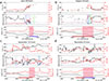 |
Figure 1 (a)–(d) The variation in the solar wind velocity (V), density (N), subsolar distance of the model magnetopause, dynamic pressure (Pd), SYM-H and ASYM-H during each Japan aurora event. The subsolar distance of the magnetopause was calculated using OMNI2 solar wind data using the model of Shue et al. (1998). Blue shaded regions denote modeled GMC events, green shaded regions denote observed GMC events by GOES satellites, and red shaded regions denote the time periods when red auroras were observed by citizen scientists in Japan. Red and blue bars describe the time interval of calculated median value of V, N and Pd described in Table 1. |
We firstly focus on GROUP 1 events to describe the auroral appearance during moderately intense storms driven by CME. The peak Dst index for GROUP 1 events ranged from −100 to −121 nT. These events were associated with intense magnetospheric compression as indicated by the small magnetopause distance (6−7 RE). These auroras were too faint to see with the naked eye. Note that, red auroras on August 4 and September 12 were not observed at Nagoya University’s aurora observatories in Rikubetsu (Eastern Hokkaido, 43.5° N, 143.8° E, 36.9° MLAT) and Moshiri (Northern Hokkaido, 44.4° N, 142.2° E, 37.9° MLAT) due to the bad weather.
The solar wind profile indicates a particular pattern of high-density and moderate-velocity for all events. It is apparent that the high-density solar wind (16−56 /cc) or intense dynamic pressure (5−23 nPa), caused strong magnetospheric compression (5.9−7.1 RE). Interestingly, prolonged (>12 h) southward interplanetary magnetic field with Bz ranging from −5 to −20 nT, originating from CMEs contributed to storm developments (Supplementary Material, Figs. S6−S9). Note that, the speed of these CMEs ranged from 350 to 600 km/s. Three of the four storms were associated with GMC events (Supplementary Material, Fig. S5), while the November 9 event was not. However, note that, there were strong magnetospheric compression events with the smallest subsolar magnetopause range of 7–8 RE.
Figure 1 illustrates the variation in modeled subsolar magnetopause distance, solar wind dynamic pressure (Pd), density (N), and velocity (V) during the Japan aurora events. Blue shaded regions denote modeled GMC events, green shaded regions denote GMC events observed by GOES satellites, and red shaded regions denote the periods when red auroras were observed by citizen scientists in Japan. The red auroras were associated with GMC events or under the compressed magnetopause conditions, during the period of the large difference in the |SYM-H| and ASYM-H indices. Additional background information, including the solar wind drivers and geomagnetic responses for each event is provided in the next subsection and Supplementary Material, Figures S6−S9.
SYM-H and ASYM-H indices (World Data Center for Geomagnetism Kyoto et al., 2022) are derived from ground-based magnetometer observations. The SYM-H index represents the development of the symmetric ring current with higher time resolution than the Dst index, and commonly used for storm intensity evaluation. In contrast, the ASYM-H index reflects the development of partial ring current caused by outflow of ring current particle from magnetosphere. Therefore, ASYM-H index is effective to evaluate the storm intensity during intense magnetospheric compression. The relatively large ASYM-H index against |SYM-H| is consistent with the small magnetospheric size and the significant outflow of ring current particles.
2.3 Space weather context of red aurora events
2.3.1 June 28, 2024 event: The Highest Density Event
The June 28 event is “The Highest Density Event”, having the highest maximum solar wind density among the four events. The solar origin of this magnetic storm was a moderate speed CME which shock’s peak velocity is approximately 470 km/s, associated with a C3.9-class solar flare in AR13720, which occurred near the Sun’s central meridian at 2200 UT on June 25, 2024. The interplanetary shock arrived at Earth around 1020 UT on June 28. Before the shock’s arrival, the SBZ (southward interplanetary magnetic field) of approximately −10 nT prolonged more than 20 hours, and it contributed the gradual development of the magnetic storm (Supplementary Material, Fig. S6). After shock’s arrival, highly compressed solar wind and strong SBZ of approximately −20 nT triggered further development of the storm. The Kp index reached 8− between 1200 UT and 1500 UT. Around 1200 UT, a high-density structure arrived, and the solar wind density increased to a high level of 60–70 /cc. During this period, the magnetopause experienced strong compression in the Shue model, with the minimum of approximately 6 RE, and GMC occurred between 1407–1426 UT at GOES 16 (Supplementary Material, Fig. S5a). The red aurora appeared during the GMC event (Fig. 1). Further details are provided in Supplementary Material, Figure S6.
2.3.2 August 4, 2024 event: the long GMC and undefined CME event
The August 4 event is “Long GMC” and an “Undefined CME” event. This storm featured the longest GMC duration of the four events, lasting over two hours. The solar origin was a moderate speed CME, which shock’s peak velocity is approximately 400 km/s, and its exact source remains unclear. At approximately 0640 UT on August 4, a CME-related interplanetary shock arrived at Earth. The highly compressed solar wind and continuous SBZ (>12 h, ~−10 nT) downstream of the shock contributed to the storm development, with the Kp index reaching 7 between 1500 and 1800 UT. As high-density structure (40–60 /cc) downstream of the shock passed, the magnetopause experienced strong compression in the Shue model, with the minimum of approximately 6.5 RE, and GMCs intermittently occurred between 1440 and 1700 UT at GOES 16 (Supplementary Material, Fig. S5b). The red aurora appeared during GMC events (Fig. 1). Further details are provided in Supplementary Material, Figure S7.
2.3.3 September 12, 2024 event: The Akita Aurora event
The September 12 event is “The Akita Aurora Event” because it was the only case among the four in which a red aurora was observed from Akita prefecture, located in northern main island, Japan. This event involved two interplanetary shocks. The first interplanetary CME-related shock arrived at Earth around 0610 UT on September 12, followed by a second shock at 1200 UT. One of the storm’s solar origins was a CME associated with a M1.2-class solar flare in AR13814, located in the northern part of the central solar meridian, at 0000 UT on September 10, 2024. However, the source of the other remains uncertain. The highly compressed solar wind and strong SBZ (~−15 nT) downstream of the shock contributes to the storm development, with the Kp index reaching 7− between 0900 and 1500 UT, and 7, between 1800 and 2100 UT. After the second shock’s arrival, a high-density structure (~40 /cc) passed, and the magnetopause experienced strong compression in the Shue model, with the minimum of approximately 6 RE, between 0910 and 1020 UT. Additionally, GMC event occurred between 1830 and 1920 UT at both GOES 16 and GOES 18 satellites (Supplementary Material, Fig. S5c). The red aurora appeared during intense magnetospheric compression events (Fig. 1). Further details are provided in Supplementary Material, Figure S8.
2.3.4 November 9, 2024 event: Without GMC Event
The November 9 storm is “without a GMC event,” as it was the only event among the four that was not associated with GMC events (Supplementary Material, Fig. S5d). The solar origin of this magnetic storm was a faint, moderate speed CME, which shock’s peak velocity is approximately 400 km/s, associated with an X2.3-class solar flare in AR13883, located in the southern part of the central solar meridian, at 1300 UT on November 6, 2024. The associated CME was not visible in coronagraph images. The associated interplanetary shock arrived at Earth around 1100 UT on November 8. The prolonged SBZ (> 18 h, ~−10 nT) downstream of the shock led to the gradual development of a geomagnetic storm, with the Kp index reaching 5 between 1200 and 1500 UT on November 9. At 0930 UT, the passage of a high-density structure (~30 /cc) compressed the magnetosphere, reaching approximately 7 RE in the Shue model by 1000 UT. Between 1300 and 1400 UT, another high-density structure (30–40 /cc) passed, however, Bz remained near zero, and the magnetospheric compression stayed at about 8 RE. The appearance of the red aurora corresponded to strong magnetospheric compression and the passage of high-density structures (Fig. 1). Further details are provided in Supplementary Material, Figure S9.
2.3.5 March 26, 2025 event: CIR driven event
CMEs are usually dominant in producing large magnetic storms with low-latitude auroras. CIR-driven low-latitude auroral events are relatively rare, although CIRs can sometimes drive large storms (Richardson et al., 2006). Note that, Shiokawa et al. (2001, 2005) first reported a CIR-related low-latitude auroral event, which occurred on May 13, 1999. We report another red aurora event associated with CIR which occurred on March 26, 2025. The solar origin of this storm is composed by two sources. One of the origins is the CIR associated with a coronal hole. The other is CMEs which passed the Earth on March 24, 2025. The peak Bt and Bz of this disturbance is strong (Bt ≈ 22 nT, Bz ≈ −20 nT), indicating that the CIR was affected by the aftermath of the CMEs. Furthermore, between 1332 UT to 1341 UT, GMC events intermittently occurred at the GOES 16 satellite (Supplementary Material, Fig. S5e), indicating that the red aurora appeared during the intense magnetospheric compression conditions. The GMC events were caused by the intense dynamic pressure due to the passing of the high-density solar wind (> 30 /cc). Further details are provided in Supplementary Material, Figure S14.
3 Method of analysis
To roughly estimate the auroral altitude from the citizen science photographs, we must rely on several different assumptions. In this study, we firstly assume that the red aurora in the photograph approximately represents the altitude profile of the auroral emission at the equatorward boundary of the auroral oval. The actual emission distribution cannot be fully resolved because auroral photographs provide only two-dimensional, line-of-sight integrated information, while the auroral oval has latitudinal width. Secondly, since all of the auroral appearances were at low elevation angles, we treat the equatorward boundary as a “flat plane” that follows the local magnetic dip angle at the equatorward boundary, while neglecting the curvature of the magnetic field lines.
Based on the International Geomagnetic Reference Field (IGRF) model (Alken et al., 2021), we identified the relevant magnetic field line at the satellite’s position when it observed the equatorward boundary of the electron precipitation. We then calculated the magnetic dip angle individually for each event at the satellite’s position (satellite’s latitude, 142°E, altitude of 850 km). We approximated the magnetic field line as a straight line with this calculated dip angle, extending it upwards and downwards from the spacecraft position. Note that the satellite altitudes change only approximately 20 km, and the error caused by the variation can be negligible for this study. The solid black line in Figure 2a shows the magnetic field line for the representative event of August 4.
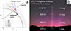 |
Figure 2 Estimation of auroral altitude using photograph taken by citizen scientist and satellite-derived magnetic field line. (a) The magnetic field line of the satellite location (red marker) is shown by black solid line. The lines-of-sight of 0-, 10-, 20-, 30-degree elevation angles are shown by red, green, blue, magenta solid lines. Each estimated altitude is indicated by the corresponding dotted curve, with altitudes of 220 km, 480 km, 800 km, and 1110 km. (b) The altitude distribution of auroral emission was visualized by superimposing an altitude grid on the photograph. |
Using this setup, we first measured the elevation angles of the auroral body from the photographs with reference to background stars. Next, we projected the lines-of-sight at the measured elevation angle onto the magnetic field line corresponding to the equatorward boundary of the auroral oval, as derived from satellite data (Fig. 2a). Finally, we superimposed the grids representing the estimated altitude on the original photograph, and visualized the altitude distribution of auroral emission (Fig. 2b).
Note that, the auroral top boundary has gradual distribution tail, and the appearance of the auroras can be contaminated under moonlit conditions etc. Additionally, the actual auroral top is too faint to be detected by cameras. Therefore, we focus on visualizing the auroral altitude distribution by simply superimposing the scale onto the photograph.
At 1346–1350 UT, when auroras were observed in Hokkaido, the NOAA18 satellite was located at near Japan’s meridian, i.e. 48–65°N and 124–113°E at that time. At 1348 UT, the equatorward boundary of the auroral oval was located at 57.9°N, 119.2°E. (Supplementary Material, Fig. S2).
Using the magnetic dip angle along the 142 °E longitude line passing through central Hokkaido, and the magnetic field line identified at 57.9 °N from NOAA18 observations, we plotted the magnetic field line, as shown in Figure 2a. Consequently, we estimate that the auroral body at an elevation angle of 20° reached an altitude of ~800 km at 1659 UT.
There are two primary sources of error for the altitude estimation. First, the altitude grids have uncertainties due to non-synchronous observations. The variation in auroral elevation angle within each photograph can cause uncertainties. The photographs analyzed in this study represent the timing of typical auroral conditions when the elevation angles of the auroral body was at its maximum for each event. However, the observation times of the aurora and the satellite passes are not exactly synchronized. Therefore, we have to consider the potential error caused by the time difference between photograph and satellite observations. In this case, the time difference is the largest, exceeding three hours, and the elevation angles of the auroral body roughly changed by approximately 15 degrees (from 20° to 5°) during the three hours time interval. Consequently, the estimated altitude of this case can be ~450 km lower. In contrast, the events on June 28, 2024; September 12, 2024; November 9, 2024; and March 26, 2025 had shorter time difference around 20 minutes. The variation in elevation angle of the auroral upper edge over these shorter intervals is limited to approximately 3 degrees (from ~12° to ~9°), and their altitude can be about ~110 km lower.
Second, the latitudinal width of the auroral oval can also cause uncertainties. We cannot definitively determine which rayed structure in the photograph corresponds to a specific magnetic field line. Auroral oval has a latitudinal width in the polar direction but the auroral photographs only serve two-dimensional information. If the selected rayed structure is located three degrees poleward, the auroral height can be about 170 km above at the elevation angle of 10° in this case. Similar uncertainties (~150 km, at elevation angle of 10°) were found in the other cases.
4 Results
4.1 June 28 event
Between 1300 and 1530 UT on June 28, 2024, citizen scientists in Hokkaido successfully observed red auroras. At this time, the peak Dst index was −107 nT at 1300 UT, and the auroras appeared during both the main phase and the recovery phase of the magnetic storm. Based on photographs taken by TN, the aurora exhibited dynamically changing red aurora with faint longitudinal structure, which is the characteristic of storm-time substorms (Fig. 3b). Note that, all photographs exhibited diffuse auroral emission, therefore there is a possibility of mixture of red aurora and SAR arc. Figure 3a shows the locations where citizen scientists observed the auroras, while Figures 3c and 3d present the representative photographs taken by citizen scientist and TN. Note that the number of citizen scientist who observed this aurora is the highest among the five events we report in this section.
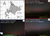 |
Figure 3 The locations of observation by citizen scientists and the red aurora photographs. (a) The locations of observation of red aurora. (b) Yoichi, Hokkaido (43.3°N, 140.7°E; red marker), Japan at 1354 UT (2254 JST, Japan local time) on 28 June 2024. (Courtesy of TN); (c) Nayoro, Hokkaido (44.4°N, 142.4°E; blue marker), at 1410 UT (Courtesy of Y. Sano); (d) Yoichi, Hokkaido (43.3°N, 140.7°E; red marker), Japan at 1424 UT (2324 JST, Japan local time) on 28 June 2024. (Courtesy of TN). |
At 1448–1452 UT, when auroras were observed in Hokkaido, the NOAA18 satellite orbited at near Japan’s meridian, i.e. 50–64°N and 108–99°E. At 1450 UT, we estimate the equatorward boundary of the auroral oval to be located at 56.6°N, 104.2°E (Supporting Information, Fig. S1).
Consequently, we estimate that at 1424 UT, the upper portion of the aurora where the aurora transitioned from reddish-purple to blue – probably caused by resonant scattering (e.g., Kataoka et al., 2024b) – reached an altitude of ~650 km at an elevation angle of 14° (Fig. 4). The figure of the workflow of the altitude estimation is provided in Supplementary Material, Figure S4a.
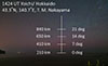 |
Figure 4 The estimation of the auroral altitude of June 28 event. The elevation angles of the auroral body were derived from the photograph, using stars as reference points, and then mapped onto the image. These angles were projected onto the magnetic field line at the equatorward boundary of the auroral oval, as estimated from satellite observation. As a result, the altitude of upper portion of the aurora was estimated to be ~650 km at an elevation angle of 14°. |
4.2 August 4 event
Between 1145 and 1800 UT on August 4, 2024, citizen scientists in Hokkaido successfully observed magenta auroras. At that time, the peak Dst index was −100 nT at 1800 UT, and the auroras appeared during the main phase of the magnetic storm. Based on the photographs taken by citizen scientists, the auroras displayed clear rayed structures. These auroras appeared due to storm-time substorms.
Additionally, between 1650 and 1800 UT, tall blue auroras exceeding the elevation angle of 30°, probably associated with N2+ resonant scattering (e.g., Kataoka et al., 2024), were also observed (Fig. 5b). Figure 5a shows the observation locations of aurora in Hokkaido, and Figures 5b–5d present the magenta aurora photographs taken by citizen scientists. Although the number of observations by citizen scientists was the lowest among the five events due to bad weather, the observation was successful thanks to widely distributed citizen science network.
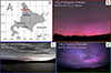 |
Figure 5 The locations of observation by citizen scientists and the magenta aurora photographs. (a) The locations of observation of magenta aurora. (b) Nakagawa, Hokkaido (44.8°N, 142.1°E), Japan at 1702 UT (0202 JST, 5 August, Japan local time) on 4 August 2024. (Courtesy of K. Tamura); (c) Shibetsu, Hokkaido (44.2°N, 142.5°E), at 1221 UT (Courtesy of T. Kato); (d) Hobetsu, Hokkaido (42.8°N, 142.2°E), at 1704 UT (Courtesy of K. Uematsu). |
As mentioned in Section 3, at 1659 UT, we estimate that the upper portion of the aurora where the aurora transit from reddish-purple to the gray sky background, at an elevation angle of 20 degrees, reached an altitude of ~800 km.
4.3 September 12 event
Between 1300 UT and 1615 UT on September 12, 2024, citizen scientists in Hokkaido and Akita prefecture successfully observed magenta auroras. The peak Dst index was −121 nT at 1500 UT, and the auroras appeared during the main phase of the magnetic storm. Based on the photographs taken by citizen scientists, the auroras exhibited dynamically changing red aurora with faint longitudinal structure (Fig. 6b). In other photographs (Figs. 6c–6e), there are diffuse red auroras, indicating the possible mixture of red aurora and SAR arc. These auroras appeared due to storm-time substorms. Figure 6a shows the observation locations of aurora in the northernmost part of Japan, and Figures 6b–6e show the magenta aurora photographs taken by TN and citizen scientists.
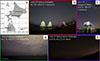 |
Figure 6 The locations of observation by citizen scientists and the auroral photographs. (a) The locations of observation of magenta aurora. (b) Setana, Hokkaido (42.5°N, 139.8°E), Japan at 1345 UT (2245 JST, Japan local time) on 12 September 2024. (Courtesy of T. Yamauchi); (c) Katagami, Akita (39.9°N, 140.0°E), at 1419 UT (Courtesy of Y. Kodama); (d) Otaru, Hokkaido (43.2°N, 141.0°E), at 1602 UT (Courtesy of TN); (e) Noboribetsu, Hokkaido (42.6°N, 141.1°E), at 1345 UT (Courtesy of R. Satoh). |
Between 1358 UT and 1402 UT, when auroras were observed in Hokkaido, the NOAA18 satellite was located at Japan’s meridian, i.e. 50–64°N and 120–112°E. The equatorward boundary of the auroral oval was estimated to be located at 58.0°N, 116.3°E at 1400 UT (Supplementary Material, Fig. S3).
Consequently, we estimate that at 1345 UT, the upper portion of the aurora where it transitioned from magenta to gray reached an altitude of ~630 km at an elevation angle of 10° (Fig. 7). The figure of the workflow of the altitude estimation is provided in Supplementary Material, Figure S4b.
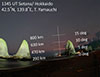 |
Figure 7 The estimation of the auroral altitude of September 12 event. The elevation angles of the auroral body were derived from the photograph, using stars as reference points, and then mapped onto the image. These angles were projected onto the magnetic field line at the equatorward boundary of the auroral oval, as estimated from satellite observation. As a result, the altitude of the upper portion of the aurora was estimated to be ~630 km at an elevation angle of 10°. |
4.4 November 9 event
Between 1210 UT and 1800 UT on November 9, 2024, citizen scientists in Hokkaido successfully observed red auroras. The peak Dst index was −101 nT at 1300 UT, and the auroras appeared during both the main phase and the recovery phase of the geomagnetic storm. Based on photographs taken by TN, the auroras displayed clear rayed structures, and appeared due to storm-time substorms. Figure 8a shows the observation locations of aurora in Hokkaido, Figures 8b and 8d presents the red aurora photograph taken by TN, while Figure 8c presents the diffuse red aurora photograph taken by citizen scientist. Therefore, possible mixture of red aurora and SAR arcs is present throughout the auroral occurrence period.
 |
Figure 8 The locations of observation by citizen scientists and the red aurora photographs taken by citizen scientists. (a) The locations of observation of red aurora. (b) Otaru, Hokkaido (43.2°N, 141.0°E), Japan at 1222 UT (2122 JST, Japan local time) on 9 November 2024. (Courtesy of TN); (c) Hobetsu, Hokkaido (42.8°N, 142.2°E), at 1359 UT (Courtesy of K. Uematsu); (d) Otaru, Hokkaido (43.2°N, 141.0°E), at 1428 UT (Courtesy of TN). |
Fortunately, MetOp3 and NOAA18 passed near Japan’s meridian during the beginning and the end of the substorm. MetOp3 observed the auroral oval before the substorm, while NOAA18 observed the expanded auroral oval after the substorm.
At 1205–1210 UT, when the auroral appearance in Hokkaido started, the MetOp3 satellite was orbiting at near Japan’s meridian, i.e. 48–65°N and 132–121°E. We estimate the equatorward boundary of the auroral oval was located at 59.1°N, 126.0°E at 1208 UT (Fig. 9).
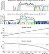 |
Figure 9 MetOp3 satellite TED and MEPED data across the auroral oval for the time interval from 1205UT to 1215 UT, November 9, 2024. The energies of TED electron differential fluxes are 189, 844, 2,595, and 7,980 eV as colored by black, blue, green, and red, respectively. The energies of MEPED proton differential fluxes are 39, 115, 332, 1105, and 2723 keV as colored by black, blue, green, red and yellow, respectively. The MetOp3 satellite was located at near Japan’s meridian, i.e. 48–65°N and 132–121°E at that time. The location where the flux of 189 eV electron (black line) exceeds 103/cm2-s-sr-eV level is identified as the equatorward boundary of the auroral oval. In this case, the timing is 1208 UT, and the geographic coordinate is 59.1°N, 126.0°E. |
Similarly, at 1328–1332 UT, when auroras were observed from Hokkaido, the NOAA18 satellite was orbiting at near Japan’s meridian, i.e. 51–65°N and 128–119°E. We estimate that the equatorward boundary of the auroral oval was located at 57.3°N, 124.5°E at 1330 UT (Fig. 10).
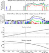 |
Figure 10 NOAA18 satellite TED and MEPED data across the auroral oval for the time interval from 1328 UT to 1332 UT, November 9, 2024. The energies of TED electron differential fluxes are 189, 844, 2,595, and 7,980 eV as colored by black, blue, green, and red, respectively. The energies of MEPED proton differential fluxes are 39, 115, 332, 1105, and 2723 keV as colored by black, blue, green, red and yellow, respectively. The NOAA18 satellite was located at near Japan’s meridian, i.e. 51–65°N and 128–119°E at that time. The location where the flux of 189 eV electron (black line) exceeds 103/cm2-s-sr-eV level is identified as the equatorward boundary of the auroral oval. In this case, the timing is 1330 UT, and the geographic coordinate is 57.3°N, 124.5°E. |
Consequently, we estimate that at 1222 UT, the upper portion of the aurora where it transitioned from red to blue was estimated to have reached an altitude of ~490–~570 km at an elevation angle of 8° (Fig. 11).
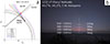 |
Figure 11 Estimation of auroral altitude of November 9 event. (a) The magnetic field line of the MetOp3 satellite’s location (red marker) is shown by black solid line. Black dotted line is the magnetic field line at 57.3°N derived from NOAA18 satellite. The black marker is the location of the observation. The lines-of-sight of 0-, 4-, 8- and 12-degree elevation angles are shown by red, green, blue, magenta solid lines. Each estimated altitude is indicated by the corresponding dotted curve, with altitudes of 310 km, 440 km, 570 km, and 710 km. (b) The resulting auroral altitude (~490 – ~570 km) was visualized by superimposing an altitude grid on the photograph. |
4.5 CIR driven auroral event on March 26, 2025
Between 1318 UT and 1420 UT on March 26, 2025, citizen scientists in Hokkaido successfully observed red auroras. The peak Dst index was only −62 nT at 2100 UT, and the auroras appeared during the beginning stage of the geomagnetic storm. Based on citizen science photographs, the aurora exhibited clear rayed structures which are characteristic of storm-time substorms. Figure 12a shows the observation locations of aurora in Hokkaido, and Figures 12b–12d present the red aurora photographs taken by citizen scientists.
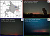 |
Figure 12 The locations of observation by citizen scientists and the red aurora photographs taken by citizen scientists. (a) The locations of observation of red aurora. (b) Kushiro, Hokkaido (43.1°N, 144.5°E), Japan at 1334 UT (2234 JST, Japan local time) on 26 March 2025. (Courtesy of K. Yajima); (c) Kitami, Hokkaido (43.8°N, 143.8°E), at 1338 UT (Courtesy of M. Hombo); (d) Teuri Island, Hokkaido (44.4°N, 141.3°E), at 1322 UT (Courtesy of K. Imahori). |
Fortunately, two satellites, MetOp3 and NOAA18, passed near Japan’s meridian before and after the red auroral appearance in Hokkaido. MetOp3 observed the auroral oval before the substorm, while NOAA18 observed the expanded auroral oval after the substorm.
At 1312–1317 UT, before the auroral appearance, the MetOp3 satellite orbited near Japan’s meridian, i.e. 50–67°N and 113–101°E. We estimate that the equatorward boundary of the auroral oval was located at 62.4°N, 107.0°E at 1315 UT (Fig. 13).
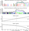 |
Figure 13 MetOp3 satellite TED and MEPED data across the auroral oval for the time interval from 1312 UT to 1317 UT, March 26, 2025. The energies of TED electron differential fluxes are 189, 844, 2,595, and 7,980 eV as colored by black, blue, green, and red, respectively. The energies of MEPED proton differential fluxes are 39, 115, 332, 1105, and 2723 keV as colored by black, blue, green, red and yellow, respectively. The MetOp3 satellite was located at near Japan’s meridian, i.e. 50–67°N and 113–101°E at that time. The location where the flux of 189 eV electron (black line) exceeds 103/cm2-s-sr-eV level is identified as the equatorward boundary of the auroral oval. In this case, the timing is 1315 UT, and the geographic coordinate is 62.4°N, 107.0°E. |
Additionally, in the end of auroral appearance, at 1430–1435 UT, the NOAA18 satellite passed near Japan’s meridian, i.e. 52–69°N and 112–98°E. We estimate that the equatorward boundary of the auroral oval was located at 58.6°N, 109.0°E at 1431 UT (Fig. 14). To consider the expanding condition of auroral oval, we used both equatorward boundaries.
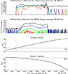 |
Figure 14 NOAA18 satellite TED and MEPED data across the auroral oval for the time interval from 1430 UT to 1435 UT, March 26, 2025. The energies of TED electron differential fluxes are 189, 844, 2,595, and 7,980 eV as colored by black, blue, green, and red, respectively. The energies of MEPED proton differential fluxes are 39, 115, 332, 1105, and 2723 keV as colored by black, blue, green, red and yellow, respectively. The NOAA18 satellite was located at near Japan’s meridian, i.e. 52–69°N and 112–98°E at that time. The location where the flux of 189 eV electron (black line) exceeds 103/cm2-s-sr-eV level is identified as the equatorward boundary of the auroral oval. In this case, the timing is 1431 UT, and the geographic coordinate is 58.6°N, 109.0°E. |
We estimate that at 1334 UT, the upper portion of the aurora where the aurora transitioned from red to gray reached an altitude of ~550 to ~750 km at an elevation angle of 8° (Fig. 15).
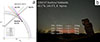 |
Figure 15 The estimation of auroral altitude of March 26, 2025 event. (a) The magnetic field line of the NOAA18 satellite’s location (red marker) is shown by black solid line. Black dotted line is the magnetic field line at 62.4°N derived from MetOp3 satellite. The black marker is the location of the observation. The lines-of-sight of 0-, 4-, 8-, 12-degree elevation angles are shown by red, green, blue, magenta solid lines. Each estimated altitude is indicated by the corresponding dotted curve, with altitudes of 300 km, 410 km, 550 km, and 700 km. (b) The resulting auroral altitude was visualized by superimposing an altitude grid on the photograph. |
5 Discussions
5.1 The actual intensity of the storms
We discuss possible mechanisms to explain the appearance of red auroras in Hokkaido, Japan during “moderately intense” magnetic storms. Specifically, we assess whether the amplitude of these magnetic storms was actually strong or not.
Two primary possibilities exist. The first is the effect of magnetospheric compression. Since most auroral events observed in Japan are associated with intense magnetospheric compression (Table 1), it is necessary to evaluate or subtract the contribution of dynamic pressure in the Dst index. The Dst index includes a positive contribution due to the enhancement of the Chapman-Ferraro-type magnetopause current. If the magnetospheric compression is strong, the Dst index becomes less negative, making the storm amplitude look weaker than actual.
The second possibility is the outflow of ring current particles due to a reduced magnetospheric size. When the outflow is occurring, the symmetric development of ring current is suffering, leading to an underestimation of storm amplitude based on the Dst and SYM-H indices. The actual development of the ring current is then better represented in the partial ring current rather than in the symmetric index. That aspect can be evaluated by comparing the SYM-H and ASYM-H indices. Note that, Kataoka et al. (2024a) indicated the importance of the large difference between the |SYM-H| and ASYM-H indices during the storm, however multi-event analysis has never been conducted.
To evaluate the contribution of the first possibility, we calculated the pressure-corrected Dst index (Dst*), with the results presented in Table 1. The Dst* values for GROUP 1 were approximately 4–15 nT greater than the Dst index, with the June 28 and August 4 events showing significantly larger differences. However, the amplitudes of the other two magnetic storms in GROUP 1 were not particularly large when considering only Dst*. The Dst* amplitudes of the storms of GROUP2 and 3 were comparable to their respective Dst values. More detailed information is provided in Supplementary Material, Figure S15.
To assess the contribution of the second possibility, we show the solar wind density (N), solar wind speed (V), dynamic pressure (Pd), subsolar distance of magnetopause, and the SYM-H and ASYM-H indices for each storm in Figure 1 (GROUP 1 storms) and Figure 16 (GROUP 2 and 3 storms).
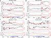 |
Figure 16 (a)–(d) The variation in the solar wind velocity (V), density (N), subsolar distance of the magnetopause, dynamic pressure (Pd), SYM-H and ASYM-H during magnetic storms in GROUP 2 (a, b) and 3 (c, d). Blue shaded regions denote modeled GMC events, green shaded regions indicate GMC events observed by GOES satellites. Red and blue bars describe the time interval of calculated median value of V, N and Pd described in Table 1. |
The actual storm amplitude shown by the ASYM-H index of GROUP 1 storms was significantly larger than it looked like from the amplitude of Dst* index. Also, the ASYM-H index of GROUP 1 storms was approximately 1.5 times greater than the peak of |SYM-H|. The enhanced ASYM-H index reflects the development of the partial ring current due to the reduced magnetospheric size. In contrast, the value of ASYM-H minus |SYM-H| for GROUP 3 storms was small or even negative. These results suggest that the first possibility had only a marginal effect, while the second possibility, namely the outflow of ring current particles from the magnetosphere due to a reduced magnetospheric size, appears to be the primary factor.
Additionally, we emphasize the need to examine the effect of dynamic pressure in more detail to see whether its primary driver is solar wind density or speed. In GROUP 1, the ASYM-H index remained high throughout the storm, and the appearance of red auroras corresponded to the significant difference between ASYM-H and |SYM-H| and the passing of high density structures. In contrast, red auroras did not appear during GROUP 2 storms with relatively low solar wind density even though the dynamic pressure is large due to the high speed. We further discuss this point in the following subsection.
5.2 The effect of solar wind density on low-latitude aurora
Here we attempt to highlight the potential importance of solar wind density, as a third critical parameter in monitoring magnetic storms to predict the low latitude auroral appearance and the thermospheric density enhancement, alongside SBZ and solar wind speed. Our results shown in the previous subsection can underscore the significance of solar wind density which has often been overlooked.
The process of auroral activity enhancement does not simply correlate with the intense magnetospheric compression. Samsonov et al. (2021) indicates that the intense compression can amplify both auroral and magnetospheric activities, with auroral activity intensifying approximately one hour after the onset of the intense compression. However, in GROUP 2 storms, red auroras were not observed in Hokkaido throughout the night despite these storms were associated with the intense magnetospheric compression.
To evaluate the effect of solar wind density, we compare GROUP 1 to GROUP 3 storms in Table 1. In GROUP 1 storms, the dominant factor contributing to the high dynamic pressure was the solar wind density (Fig. 1). The peak density was high, ranging from 34 to 71 /cc, while the solar wind speed was moderate, ranging from 350 to 600 km/s. In contrast, in GROUP 2, the primary driver of intense dynamic pressure was high-speed solar wind, approximately 800 km/s (Fig. 16). The peak density in GROUP 2 was about half that of GROUP 1, around 20 /cc. Similarly, in GROUP 3, the solar wind speed was comparable to GROUP 1, but the density was not high, only 10–20 /cc (Fig. 16). Here we also note that Japan’s local time coincided with the recovery phase of the October 8 storm, during which no dynamic aurora was observed. Additionally, the peak Dst index of the October 8 storm was −148 nT, greater than that of the other storms discussed, indicating different conditions from the five Japan aurora events we reported.
From the discussions above, we suggest the hypothesis that solar wind density can contribute to the enhancement of auroral activity. The storms in GROUP 1 with high-density and moderate speed were associated with Japan auroras. However, GROUP 2 storms, with the high-speed solar wind, was not associated with Japan aurora, despite the intense compression due to strong dynamic pressure. This suggests that the appearance of red auroras from Hokkaido area can correspond to the solar wind density greater than 30/cc.
5.3 Testing the hypothesis
To test the “density effect hypothesis” proposed at the previous subsection, we compare the CIR event on March 26, 2025 with GROUP 1 storms in Table 1. Additionally, we compare GROUP 1 storms with all Japan aurora event with the peak Dst index weaker than −150 nT, which occurred during the Solar Cycle 23 as reported by Shiokawa et al. (2005).
We propose that the hypothesis is consistent with the observation result of March 26 event, and can be applied to the low-latitude auroral event driven by CIR. Figure 17 shows the variation in the solar wind velocity, density and dynamic pressure obtained from OMNI2, and the SYM-H and ASYM-H indices on March 26, 2025. The solar wind density exceeded 30/cc between 08 UT to 13 UT, and the peak density was approximately 45/cc.
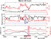 |
Figure 17 The variation in the solar wind velocity (V), density (N), dynamic pressure, the subsolar distance of modeled magnetopause, SYM-H and ASYM-H during magnetic storm on March 26, 2025. Red shaded regions represent the time periods when red auroras were observed by citizen scientists in Japan. Blue shaded regions show the time period of the subsolar distance of modeled magnetopause become smaller than 6.6 RE. Green shaded regions denote the time period of the GMC event observed by GOES 16 satellite. Red bar describes the time interval of calculated median value of V, N and Pd described in Table 1. |
The appearance of red aurora in Japan corresponded to the passage of high-density structures originating from the CIR. Furthermore, GMC events occurred during the red auroral appearance in Hokkaido. Additionally, the ASYM-H index significantly increased to 124 nT at 1408 UT during the auroral appearance. The ASYM-H amplitude was 1.7 times larger than the SYM-H index, and it is also consistent with the result of GROUP 1 events we reported.
Next, we compare GROUP 1 storms with all of the Japan aurora event with the peak Dst index weaker than −150 nT as shown by Shiokawa et al. (2005). Shiokawa et al. (2005) reported 20 red auroras observed from Japan during the Solar Cycle 23, and eight of them occurred during magnetic storms with the peak Dst index weaker than −150 nT. We check the solar wind density and velocity for these eight events.
Consequently, we propose that the simple “density effect hypothesis” is incorrect, and the relationship between auroral appearance, solar wind velocity, and density is not straightforward. The red auroral events that occurred on February 18, 1999, November 29, 2000, and April 28, 2001, as reported by Shiokawa et al. (2005), were not associated with high-density solar wind. The maximum solar wind densities for these events were 25 /cc, 12 /cc, and 25 /cc, respectively. Moreover, these events were associated with high-speed solar wind exceeding 600 km/s.
Nevertheless, we found a consistent tendency for red auroral appearances in Hokkaido to correspond with intense magnetospheric compression caused by moderate-speed and high-density ejecta. Specifically, six events with a peak Dst > −150 nT during Solar Cycle 25, and four during Solar Cycle 23, were associated with high-density (>~30 /cc), low-velocity (<600 km/s) solar wind. Furthermore, in five of the events we reported, the altitudes of the red auroras extended to ~490– ~800 km. Red auroras typically extend up to 400–600 km (Shiokawa et al., 1997; Kataoka et al., 2024a), therefore these five auroras were extremely high.
Moderate-speed and high-density ejecta can therefore trigger highly extended red auroras in midlatitude regions such as Hokkaido – even during relatively weak magnetic storms with the peak Dst index being only approximately −50 nT. These findings also suggest a possible influence of solar wind density on auroral altitudes, as all five high-altitude events occurred under slow-dense solar wind. We further discuss the possible mechanisms and directions for future studies in the next subsection.
5.4 Extension of red auroras during intense magnetospheric compression
We found that, despite the not unusual storm amplitudes, the red auroras extended to extremely high altitudes (~490 – ~800 km), accompanied by intense magnetospheric compression. The high altitude extension of red aurora is one of the contributing factors for the occurrence of red aurora in Japan.
Although this observational link is clear, the physical mechanism connecting intense magnetospheric compression and high-altitude auroras remains unclear. We suggest that atmospheric density enhancement in the upper thermosphere is essential for allowing the aurora to extend vertically. We suggest one possible mechanism that could cause atmospheric density enhancement is Joule heating associated with the magnetic storms. Robinson and Zanetti (2021) indicated that Joule heat can be the dominant mechanism of atmospheric heating, i.e., the energy from Joule heat is twice as large as the energy from particle precipitation heating during magnetic storms, on average.
Furthermore, it is necessary to elucidate the mechanism of the rapid atmospheric heating that occurs during relatively weak magnetic storms. Understanding this mechanism is essential for predicting unexpected atmospheric drag enhancement on satellites. We emphasize that the highly extended red aurora on March 26, 2025 (~550 km – ~750 km) appeared in the early stage of the magnetic storm, with the Dst index of only −48 nT (14 UT). It is a different condition from the other four storms.
Kataoka et al. (2025) proposed that the appearance of red aurora in Japan during the early stage of the magnetic storm on October 10, 2024 corresponded to the super substorm with the peak AE index (World Data Center for Geomagnetism Kyoto et al., 2015a) larger than 4,000 nT. However, the peak AE index during the auroral appearance on March 26, 2025 was only 600–1,000 nT, indicating the substorms were not so great.
The preheating due to the previous magnetic storm may contribute to the thermospheric density enhancement and auroral appearance in Hokkaido during the early stage of the storm. In fact, 11 hours before of the red aurora appearance in Hokkaido on March 26, 2025, another weak magnetic storm with the peak Dst index of −60 nT occurred. However, it is not realistic to evaluate the contribution of preheating to auroral appearances due to the limitation of atmospheric heating model, therefore; this topic beyonds the scope of our study.
The underlying mechanism behind the relationship between the high-altitude extension of red auroras driven by atmospheric heating and intense magnetospheric compression, which can lead to GMC events, remains unclear. We here suggest that more detailed, physics-based dynamic modeling studies are necessary not only for great storms but also for the relatively moderate storms. However, such a modeling is not straightforward because the upper boundaries of the simulation models are often set to be ~600 km. This is an urgent issue for the study of atmospheric drag on satellites, particularly for mitigating space weather hazards, such as the unexpected reentry of LEO satellites (Hapgood et al., 2022; Kataoka et al., 2022).
5.5 Further discussions
Note that there is another factor possibly contributing to the occurrence of red auroras in Hokkaido. While the yearly shift in the MLAT of Hokkaido’s meridian is small, it can be a contributing factor. In fact, the MLAT of Japan’s meridian has shifted approximately 0.4 degrees (~44 km) to higher latitudes, based on the rate of change in MLAT for Sapporo over the past 20 years (Solar Cycle 23–25) using the Altitude Adjusted Corrected GeoMagnetic (AACGM) v2 model (Shepherd, 2014).
Finally, we repeatedly emphasize the advantage of citizen science. The super dense network over Japan, especially Hokkaido, ensures that aurora events are rarely missed. The extensive auroral observation network established by spreading citizen scientists can even capture irregular encounter of aurora. In fact, the red aurora events on August 4 and September 12 were not observed by Nagoya University’s observatories in Rikubetsu and Moshiri, Hokkaido.
In addition to this spatial coverage, recent technological advancements have further increased the value of citizen science. High-sensitive and high-resolution auroral photographs provided by citizen scientists have enabled the estimation of auroral altitudes for multiple events. For comparison, Shiokawa et al. (2005) could not determine auroral heights due to the low resolution of available all-sky photographs.
Although our findings contribute to the understanding of low latitude aurora, the underlying mechanism behind the relationship between extended red aurora and intense magnetospheric compression remains unelucidated. Further global modeling studies are needed to fully understand the exact mechanisms. This multi-event study is of course far from the statistical study, and we wish further continuous and intensive observation activities of low-latitude aurora will enable a conclusive statistical study in future.
6 Conclusions
We reported four low-latitude auroral events observed from Hokkaido, Japan, on June 28, August 4, September 12, November 9, 2024. Additionally, we also reported one CIR-driven low-latitude auroral event on March 26, 2025. All of these events occurred during moderately intense or weak magnetic storms, accompanied by significant magnetospheric compression. During the appearance of red auroras in Japan, the ASYM-H index increased approximately 1.3–2.0 times larger than the SYM-H peak amplitude in all events, indicating that the actual development of these storms was larger than the implication by the Dst and SYM-H indices. We found that the altitude of the red aurora is extremely high (~490 km – ~800 km), accompanied by intense magnetospheric compression such as GMC events.
Acknowledgments
We greatly acknowledge Prof. Nozomu Nishitani and Dr. Naritoshi Kitamura for their valuable advice, which greatly contributed to this research. The continuous observations of low-latitude aurora from Hokkaido have been conducted by the cooperation with many members of the Hokkaido University Astronomy Club, including T. Asada, D. Kato, Y. Kamiyama, S. Watanabe, Y. Era, H. Kuwabara, Y. Sasaki, S. Itoi, T. Sugioka, H. Komori, M. Shiratori, Y. Fujise, R. Washio, Y. Kato, A. Suzuki, R. Maeno, Y. Murata, S. Imoto, T. Ando, A. Uno, K. Onaru, Y. Kato, R. Kobayashi, Y. Nishino, Y. Bando, Y. Miyoshi, K. Ebe, K. Onogi, S. Sato, F. Takamatsu, Y. Nakamura and T. Nishizaki. We much appreciate their great support during observation workshops in Hokkaido since November 2021. We also appreciate the discussion of the aurora data and the mechanism of the auroral appearance with them. Furthermore, we greatly acknowledge the great effort of citizen scientists who have conducted continuous observation of low-latitude aurora throughout Solar Cycle 25 including K. Tamura, S. Fukushima, Y. Sano, T. Kato, K. Uematsu, A. Takimoto, K. Imahori, K. Yajima, M. Hombo, T. Ikeda, T. Yamauchi, R. Satoh, Y. Kodama, K. Tomita, H. Saitou, J. Morimoto and Satoru. C. The editor thanks two anonymous reviewers for their assistance in evaluating this paper.
Funding
TN is supported by Hokkaido University Astronomy Club. RK is supported by JSPS KAKENHI 24H00277, Hoso Bunka Foundation and NIJL DDH project.
Data availability statement
The OMNI2 5-min data was obtained from the OMNIWeb (https://omniweb.gsfc.nasa.gov/ow_min.html). The Provisional Dst index, SYM-H index, ASYM-H index and AE index were provided by the WDC for Geomagnetism, Kyoto (http://wdc.kugi.kyoto-u.ac.jp/wdc/Sec3.html). The NOAA 18, MetOp 3 TED and MEPED data were obtained from CDA Web (https://cdaweb.gsfc.nasa.gov/). GOES 16 and 18 magnetometer data were also obtained from CDA Web. The intensity data of aurora were obtained from the ISEE Nagoya University database (https://stdb2.isee.nagoya-u.ac.jp/omti/) The aurora maps in Figures 3, 5, 6, 8, and 12 were created using data from the National Land Numerical Information (Administrative Boundary Data) provided by the Ministry of Land, Infrastructure, Transport and Tourism (MLIT) of Japan. The dataset is available at https://nlftp.mlit.go.jp/ksj/gml/datalist/KsjTmplt-N03-v2_2.html. The grids in these maps were made with Natural Earth. Free vector and raster map data are available at https://www.naturalearthdata.com/. All of the auroral photographs taken by TN and citizen scientists are available on X/Twitter, with the hashtag of “aurora citizen” in Japanese.
Supplementary material
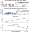 |
Figure S1. NOAA18 satellite TED and MEPED data across the auroral oval for the time interval from 1448 UT to 1452 UT, June 28, 2024. The energies of TED electron differential fluxes are 189, 844, 2,595, and 7,980 eV as colored by black, blue, green, and red, respectively. The energies of MEPED proton differential fluxes are 39, 115, 332, 1105, and 2723 keV as colored by black, blue, green, red and yellow, respectively. NOAA18 was located at near Japan’s meridian, i.e. 50–64°N and 108–99°E at that time. We identified the location where the flux of 189 eV electron (black line) exceeds 103 /cm2-s-sr-eV level as the equatorward boundary of the auroral oval. In this case, the timing is 1450 UT, and the geographic coordinate is 56.6°N, 104.2°E. |
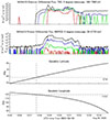 |
Figure S2. NOAA18 satellite TED and MEPED data across the auroral oval for the time interval from 1345 UT to 1350 UT, August 4, 2024. The energies of TED electron differential fluxes are 189, 844, 2,595, and 7,980 eV as colored by black, blue, green, and red, respectively. The energies of MEPED proton differential fluxes are 39, 115, 332, 1105, and 2723 keV as colored by black, blue, green, red and yellow, respectively. NOAA18 satellite was located at near Japan’s meridian, i.e. 48–65°N and 124–113°E at that time. We identified the location where the flux of 189 eV electron (black line) exceeds 103 /cm2-s-sr-eV level as the equatorward boundary of the auroral oval. In this case, the timing is 1348 UT, and the geographic coordinate is 57.9°N, 119.2°E. |
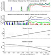 |
Figure S3. NOAA18 satellite TED and MEPED data across the auroral oval for the time interval from 1358UT to 1402 UT, September 12, 2024. The energies of TED electron differential fluxes are 189, 844, 2,595, and 7,980 eV as colored by black, blue, green, and red, respectively. The energies of MEPED proton differential fluxes are 39, 115, 332, 1105, and 2723 keV as colored by black, blue, green, red and yellow, respectively. NOAA18 satellite was located at near Japan’s meridian, i.e. 50–64°N and 120–112°E at that time. We identified the location where the flux of 189 eV electron (black line) exceeds 103 /cm2-s-sr-eV level as the equatorward boundary of the auroral oval. In this case, the timing is 1400 UT, and the geographic coordinate is 58.0°N, 116.3°E. |
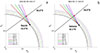 |
Figure S4. Workflow for the altitude estimation of the auroral upper edge for the June 28 and September 12 events. The magnetic field line at the location of the NOAA-18 satellite (red marker) is shown as a black solid line, while the black marker indicates the location of the observation site. The elevation angles of the auroral body were derived from photographs using stars as reference points and then projected onto the magnetic field line at the equatorward boundary of the auroral oval, as estimated from satellite data. (a) For the June 28, 2024, event observed from Yoichi (43.3°N), the lines of sight for elevation angles of 0°, 7°, 14°, and 21° are shown as red, green, blue, and magenta solid lines, respectively. Each estimated altitude is indicated by the corresponding dotted curve, with altitudes of 210 km, 410 km, 650 km, and 840 km. (b) For the September 12, 2024, event observed from Setana (42.5°N), the lines of sight for elevation angles of 0°, 5°, 10°, and 15° are shown as red, green, blue, and magenta solid lines, respectively. Each estimated altitude is indicated by the corresponding dotted curve, with altitudes of 290 km, 470 km, 630 km, and 800 km. |
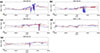 |
Figure S5. GSM Z-component of the GOES magnetometer for magnetic storm events associated with red auroras in 2024. The red lines are from GOES18, while the blue lines are fom GOES16. (a) GMC events occurred on 1407UT to 1426UT, and 1540UT to 1616UT at GOES 16. (b) GMC events occurred on 1520UT to 1645UT at GOES 16. (c) GMC occurred intermittently on 1833UT to 1918UT at GOES 16 and GOES 18. (d) GMC was not observed on November 9 event. (e) GMC events intermittently occurred on 1332 UT to 1341 UT at the GOES 16. |
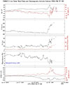 |
Figure S6. The solar wind parameters and geomagnetic activities for the June 28, 2024 storm event. From top to bottom, shown are the solar wind magnetic field strength with the southward component (red), solar wind speed, solar wind density with the dynamic pressure (red), model-esimated magnetopause distance, and the SYM-H and ASYM-H (red) indices. |
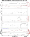 |
Figure S7. The solar wind parameters and geomagnetic activities for the August 4, 2024 storm event. From top to bottom, shown are the solar wind magnetic field strength with the southward component (red), solar wind speed, solar wind density with the dynamic pressure (red), model-esimated magnetopause distance, and the SYM-H and ASYM-H (red) indices. |
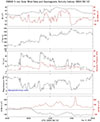 |
Figure S8. The solar wind parameters and geomagnetic activities for the September 12, 2024 storm event. From top to bottom, shown are the solar wind magnetic field strength with the southward component (red), solar wind speed, solar wind density with the dynamic pressure (red), model-esimated magnetopause distance, and the SYM-H and ASYM-H (red) indices. |
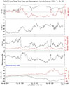 |
Figure S9. The solar wind parameters and geomagnetic activities for the November 9, 2024 storm event. From top to bottom, shown are the solar wind magnetic field strength with the southward component (red), solar wind speed, solar wind density with the dynamic pressure (red), model-esimated magnetopause distance, and the SYM-H and ASYM-H (red) indices. |
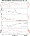 |
Figure S10. The solar wind parameters and geomagnetic activities for the November 4, 2021 storm event. From top to bottom, shown are the solar wind magnetic field strength with the southward component (red), solar wind speed, solar wind density with the dynamic pressure (red), model-esimated magnetopause distance, and the SYM-H and ASYM-H (red) indices. |
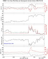 |
Figure S11. The solar wind parameters and geomagnetic activities for the March 24, 2024 storm event. From top to bottom, shown are the solar wind magnetic field strength with the southward component (red), solar wind speed, solar wind density with the dynamic pressure (red), model-esimated magnetopause distance, and the SYM-H and ASYM-H (red) indices. |
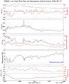 |
Figure S12. The solar wind parameters and geomagnetic activities for the September 17, 2024 storm event. From top to bottom, shown are the solar wind magnetic field strength with the southward component (red), solar wind speed, solar wind density with the dynamic pressure (red), model-esimated magnetopause distance, and the SYM-H and ASYM-H (red) indices. |
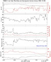 |
Figure S13. The solar wind parameters and geomagnetic activities for the October 8, 2024 storm event. From top to bottom, shown are the solar wind magnetic field strength with the southward component (red), solar wind speed, solar wind density with the dynamic pressure (red), model-esimated magnetopause distance, and the SYM-H and ASYM-H (red) indices. |
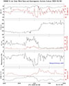 |
Figure S14. The solar wind parameters and geomagnetic activities for the March 26, 2025 storm event. From top to bottom, shown are the solar wind magnetic field strength with the southward component (red), solar wind speed, solar wind density with the dynamic pressure (red), model-esimated magnetopause distance, and the SYM-H and ASYM-H (red) indices. |
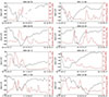 |
Figure S15. Pressure-corrected Dst index (Dst*, black) and the solar wind dynamic pressure for the all of the magnetic storm events (red) shown in this study. |
References
- Alken P, Thébault E, Beggan CD, Amit HAubert J, et al., 2021. International Geomagnetic Reference Field: the thirteenth generation. Earth Planets Space 73: 49. https://doi.org/10.1186/s40623-020-01288-x. [Google Scholar]
- Archer WE, St.-Maurice J-P, Gallardo-Lacourt B, Perry GW, Cully CM, et al., 2019. The vertical distribution of the optical emissions of a Steve and Picket Fence event. Geophys Res Lett 46: e2019GL084473. https://doi.org/10.1029/2019GL084473. [Google Scholar]
- Case NA, MacDonald EA, Heavner M, Tapia AH, Lalone N. 2015. Mapping auroral activity with Twitter. Geophys Res Lett 42: e2015GL063709. https://doi.org/10.1002/2015GL063709. [Google Scholar]
- Case NA, MacDonald EA, Viereck R. 2016. Using citizen science reports to define the equatorial extent of auroral visibility. Space Weather 14: e2015SW001320. https://doi.org/10.1002/2015SW001320. [Google Scholar]
- Cliver EW, Schrijver CJ, Shibata K, Usoskin IG. 2022. Extreme solar events. Living Rev Sol Phys 19: 2. https://doi.org/10.1007/s41116-022-00033-8. [CrossRef] [Google Scholar]
- Ebihara Y, Tanaka T, Kamiyoshikawa N. 2019. New diagnosis for energy flow from solar wind to ionosphere during substorm: Global MHD simulation. J Geophys Res Space Phys 124: 360–378. https://doi.org/10.1029/2018JA026177. [Google Scholar]
- Gonzalez WD, Joselyn JA, Kamide Y, Kroehl HW, Rostoker G, et al. 1994. What is a geomagnetic storm? J Geophys Res 99(A4): 5771–5792. https://doi.org/10.1029/93JA02867. [CrossRef] [Google Scholar]
- Grandin M, Bruus E, Ledvina VE, Partamies N, Barthelemy M, et al., 2024. The Gannon Storm: Citizen science observations during the geomagnetic superstorm of 10 May 2024. Geosci Commun 7(4): 297–316. https://doi.org/10.5194/gc-7-297-2024. [Google Scholar]
- Hapgood M, Liu H, Lugaz N. 2022. SpaceX—Sailing close to the space weather?. Space Weather 20: e2022SW003074. https://doi.org/10.1029/2022SW003074. [Google Scholar]
- Kataoka R, Iwahashi K. 2017. Inclined zenith aurora over Kyoto on 17 September 1770: Graphical evidence of extreme magnetic storm. Space Weather 15: 1314–1320. https://doi.org/10.1002/2017SW001690. [Google Scholar]
- Kataoka R, Nakano SY. 2021. Auroral zone over the last 3000 years. J Space Weather Space Clim 11: 46. https://doi.org/10.1051/swsc/2021030. [Google Scholar]
- Kataoka R, Shiota D, Fujiwara H, Jin H, Tao C, et al., 2022. Unexpected space weather causing the reentry of 38 Starlink satellites in February 2022. J Space Weather Space Clim . 12: 41. https://doi.org/10.1051/swsc/2022034. [Google Scholar]
- Kataoka R, Miyoshi Y, Shiokawa K, Nishitani N, Keika K, et al., 2024a. Magnetic storm-time red aurora as seen from Hokkaido, Japan on 1 December 2023 associated with high-density solar wind. Geophys Res Lett. 51: e2024GL108778. https://doi.org/10.1029/2024GL108778. [Google Scholar]
- Kataoka R, Reddy SA, Nakano S, Pettit J, Nakamura Y. 2024b. Extended magenta aurora as revealed by citizen science. Nat Sci Rep . 14: 25849. https://doi.org/10.1038/s41598-024-75184-9. [Google Scholar]
- Kataoka R, Nakano S, Uchino S, Sachin AR. 2025. Extended red aurora associated with super substorm igniting the October 10, 2024 magnetic storm as revealed by citizen science. Earth Planets Space . 77: 64. https://doi.org/10.1186/s40623-025-02178-w. [Google Scholar]
- Khachikjan GY, Koustov AV, Sofko GJ. 2008. Dependence of SuperDARN cross polar cap potential upon the solar wind electric field and magnetopause subsolar distance. J Geophys Res Space Phys . 113: A09214. https://doi.org/10.1029/2008JA013107. [Google Scholar]
- Kosar BC, MacDonald EA, Case NA, Zhang Y, Mitchell EJ, et al. 2018. A case study comparing citizen science aurora data with global auroral boundaries derived from satellite imagery and empirical models. J Atmos Sol-Terr Physics. 177: 274–282. https://doi.org/10.1016/j.jastp.2018.05.006. [Google Scholar]
- Li LY, Wang ZQ. 2018. The effects of solar wind dynamic pressure changes on the substorm auroras and energetic electron injections on 24 August 2005. J Geophys Res Space Phys. 123: 385–399. https://doi.org/10.1002/2017JA024628. [Google Scholar]
- Loewe CA, Prölss GW. 1997. Classification and mean behavior of magnetic storms. J Geophys Res. 102(A7): 14209–14213. https://doi.org/10.1029/96JA04020. [CrossRef] [Google Scholar]
- Ma L, Yu Y, Ding X, Liu X, An D, et al. 2024. Mid-latitude auroras and energetic particle precipitation occurred unusually in a moderate magnetic storm on 1 December 2023. Geophys Res Lett. 51: e2024GL110764. https://doi.org/10.1029/2024GL110764. [Google Scholar]
- MacDonald EA, Donovan E, Nishimura Y, Case NA, Gillies DM, et al. 2018. New science in plain sight: Citizen scientists lead to the discovery of optical structure in the upper atmosphere. Sci Adv. 4: eaaq0030. https://doi.org/10.1126/sciadv.aaq0030 [Google Scholar]
- Nakano S, Kataoka R. 2022. Echo state network model for analyzing solar-wind effects on the AU and AL indices. Ann Geophys. 40: 11–22. https://doi.org/10.5194/angeo-40-11-2022. [Google Scholar]
- Nanjo S, Shiokawa K, 2024. Spatial structures of blue low-latitude aurora observed from Japan during the extreme geomagnetic storm of May 2024. Earth Planets Space. 76 156: https://doi.org/10.1186/s40623-024-02090-9. [Google Scholar]
- Nishimura Y, Bruus E, Karvinen E, Martinis CR, Dyer A, et al. 2022. Interaction between proton aurora and stable auroral red arcs unveiled by citizen scientist photographs. J Geophys Res Space Phys. 127: e2022JA030570. https://doi.org/10.1029/2022JA030570. [Google Scholar]
- O’Brien TP, McPherron RL. 2000. An empirical phase space analysis of ring current dynamics: Solar wind control of injection and decay. J Geophys Res Space Phys. 105: 7707–7719. https://doi.org/10.1029/1998JA000437. [Google Scholar]
- Palmroth M, Grandin M, Helin M, Koski P, Oksanen A, et al. 2020. Citizen scientists discover a new auroral form: Dunes provide insight into the upper atmosphere. AGU Adv. 1: e2019AV000133. https://doi.org/10.1029/2019AV000133. [Google Scholar]
- Papitashvili NE, King JH. 2020. “OMNI 5-min Data”. NASA Space Physics Data Facility. https://doi.org/10.48322/gbpg-5r77, Accessed on April 9, 2025. [Google Scholar]
- Richardson IG, Webb DF, Zhang J, Berdichevsky DB, Biesecker DA, et al. 2006. Major geomagnetic storms (Dst ≤ −100 nT) generated by corotating interaction regions. J Geophys Res. 111: A07S09. https://doi.org/10.1029/2005JA011476 [Google Scholar]
- Robinson RM, Zanetti LJ. 2021. Auroral energy flux and Joule heating derived from global maps of field-aligned currents. Geophys Res Lett. 48: e2020GL091527. https://doi.org/10.1029/2020GL091527. [Google Scholar]
- Samsonov AA, Bogdanova YV, Branduardi-Raymont G, Xu L, Zhang J, et al. 2021. Geosynchronous magnetopause crossings and their relationships with magnetic storms and substorms. Space Weather. 19: e2020SW002704. https://doi.org/10.1029/2020SW002704 [Google Scholar]
- Shepherd SG. 2014. Altitude-adjusted corrected geomagnetic coordinates: Definition and functional approximations. J Geophys Res Space Physics 119: 7501–7521. https://doi.org/10.1002/2014JA020264. [Google Scholar]
- Semeter J, Hunnekuhl M, MacDonald E, Hirsch M, Zeller N, et al. 2020. The mysterious green streaks below STEVE. AGU Adv. 1: e2020AV000183. https://doi.org/10.1029/2020AV000183. [Google Scholar]
- Shiokawa K, Meng C-I, Reeves GD, Rich FJ, Yumoto K. 1997. A multievent study of broadband electrons observed by the DMSP satellites and their relation to red aurora observed at midlatitude stations. J Geophys Res. 102(A7): 14237–14253. https://doi.org/10.1029/97JA00741. [Google Scholar]
- Shiokawa K, Ogawa T, Oya H, Rich FJ, Yumoto K. 2001. A stable auroral red arc observed over Japan after an interval of very weak solar wind. J Geophys Res 106(A11): 26091–26101. https://doi.org/10.1029/2001JA000073. [Google Scholar]
- Shiokawa K, Ogawa T, Kamide Y. 2005. Low‐latitude auroras observed in Japan: 1999–2004. J Geophys Res Space Phys. 110: A05202. https://doi.org/10.1029/2004JA010706. [Google Scholar]
- Shue J-H, Song P, Russell CT, Steinberg JT, Chao JK, et al. 1998. Magnetopause location under extreme solar wind conditions. J Geophys Res. 103: 17691–17700. https://doi.org/10.1029/98JA01103. [Google Scholar]
- World Data Center for Geomagnetism, Kyoto NM, Iyemori T, Sugiura M, Kamei T. 2015a. Geomagnetic AE index, https://doi.org/10.17593/15031-54800, Accessed on October 23, 2025. [Google Scholar]
- World Data Center for Geomagnetism, Kyoto NM, Iyemori T, Sugiura M, Kamei T. 2015b. Geomagnetic Dst index, https://doi.org/10.17593/14515-74000, Accessed on December 16, 2025. [Google Scholar]
- World Data Center for Geomagnetism, Kyoto NM, Imajo S, Matsuoka A, Toh H, Iyemori T. 2022. Mid-latitude Geomagnetic Indices ASY and SYM (ASY/SYM Indices), https://doi.org/10.14989/267216, Accessed on October 23, 2025. [Google Scholar]
- Yang Z, Zhang B, Lei J, Dang T. 2020. Nonlinear response of the cross polar cap potential to solar wind density under northward interplanetary magnetic field. Geophys Res Lett. 47: e2020GL087559. https://doi.org/10.1029/2020GL087559. [Google Scholar]
- Yokoyama N, Kamide Y, Miyaoka H. 1998. The size of the auroral belt during magnetic storms. Ann Geophys. 16: 566–573. https://doi.org/10.1007/s00585-998-0566-z. [Google Scholar]
Cite this article as: Nakayama TM & Kataoka R, 2026. Faint red auroras as seen from Japan associated with intense magnetospheric compression. J. Space Weather Space Clim. 16, 19. https://doi.org/10.1051/swsc/2026004.
All Tables
Overview of nine magnetic storms analyzed. Four red auroral events driven by CME are summarized in GROUP 1. Magnetic storms in GROUP 2 are associated with large ASYM-H index and small magnetopause distance, and without Japan aurora. Magnetic storms in GROUP 3 are associated with moderate speed and moderate density, without large ASYM-H and dynamic aurora in Japan. The magnetic storm in GROUP 4 is associated with CIR and Japan aurora. The Dst, pressure corrected Dst (Dst*) are the minimum value throughout each storm. The minimum subsolar distance of model magnetopause, peak SYM-H and ASYM-H are calculated for the time interval of Japan’s nighttime (09 UT–21 UT). Solar wind density (N), speed (V) and dynamic pressure (Pd) are calculated for the corresponding main (red) and/or recovery (blue) phase of each storm.
All Figures
|
Figure 1 (a)–(d) The variation in the solar wind velocity (V), density (N), subsolar distance of the model magnetopause, dynamic pressure (Pd), SYM-H and ASYM-H during each Japan aurora event. The subsolar distance of the magnetopause was calculated using OMNI2 solar wind data using the model of Shue et al. (1998). Blue shaded regions denote modeled GMC events, green shaded regions denote observed GMC events by GOES satellites, and red shaded regions denote the time periods when red auroras were observed by citizen scientists in Japan. Red and blue bars describe the time interval of calculated median value of V, N and Pd described in Table 1. |
| In the text | |
|
Figure 2 Estimation of auroral altitude using photograph taken by citizen scientist and satellite-derived magnetic field line. (a) The magnetic field line of the satellite location (red marker) is shown by black solid line. The lines-of-sight of 0-, 10-, 20-, 30-degree elevation angles are shown by red, green, blue, magenta solid lines. Each estimated altitude is indicated by the corresponding dotted curve, with altitudes of 220 km, 480 km, 800 km, and 1110 km. (b) The altitude distribution of auroral emission was visualized by superimposing an altitude grid on the photograph. |
| In the text | |
|
Figure 3 The locations of observation by citizen scientists and the red aurora photographs. (a) The locations of observation of red aurora. (b) Yoichi, Hokkaido (43.3°N, 140.7°E; red marker), Japan at 1354 UT (2254 JST, Japan local time) on 28 June 2024. (Courtesy of TN); (c) Nayoro, Hokkaido (44.4°N, 142.4°E; blue marker), at 1410 UT (Courtesy of Y. Sano); (d) Yoichi, Hokkaido (43.3°N, 140.7°E; red marker), Japan at 1424 UT (2324 JST, Japan local time) on 28 June 2024. (Courtesy of TN). |
| In the text | |
|
Figure 4 The estimation of the auroral altitude of June 28 event. The elevation angles of the auroral body were derived from the photograph, using stars as reference points, and then mapped onto the image. These angles were projected onto the magnetic field line at the equatorward boundary of the auroral oval, as estimated from satellite observation. As a result, the altitude of upper portion of the aurora was estimated to be ~650 km at an elevation angle of 14°. |
| In the text | |
|
Figure 5 The locations of observation by citizen scientists and the magenta aurora photographs. (a) The locations of observation of magenta aurora. (b) Nakagawa, Hokkaido (44.8°N, 142.1°E), Japan at 1702 UT (0202 JST, 5 August, Japan local time) on 4 August 2024. (Courtesy of K. Tamura); (c) Shibetsu, Hokkaido (44.2°N, 142.5°E), at 1221 UT (Courtesy of T. Kato); (d) Hobetsu, Hokkaido (42.8°N, 142.2°E), at 1704 UT (Courtesy of K. Uematsu). |
| In the text | |
|
Figure 6 The locations of observation by citizen scientists and the auroral photographs. (a) The locations of observation of magenta aurora. (b) Setana, Hokkaido (42.5°N, 139.8°E), Japan at 1345 UT (2245 JST, Japan local time) on 12 September 2024. (Courtesy of T. Yamauchi); (c) Katagami, Akita (39.9°N, 140.0°E), at 1419 UT (Courtesy of Y. Kodama); (d) Otaru, Hokkaido (43.2°N, 141.0°E), at 1602 UT (Courtesy of TN); (e) Noboribetsu, Hokkaido (42.6°N, 141.1°E), at 1345 UT (Courtesy of R. Satoh). |
| In the text | |
|
Figure 7 The estimation of the auroral altitude of September 12 event. The elevation angles of the auroral body were derived from the photograph, using stars as reference points, and then mapped onto the image. These angles were projected onto the magnetic field line at the equatorward boundary of the auroral oval, as estimated from satellite observation. As a result, the altitude of the upper portion of the aurora was estimated to be ~630 km at an elevation angle of 10°. |
| In the text | |
|
Figure 8 The locations of observation by citizen scientists and the red aurora photographs taken by citizen scientists. (a) The locations of observation of red aurora. (b) Otaru, Hokkaido (43.2°N, 141.0°E), Japan at 1222 UT (2122 JST, Japan local time) on 9 November 2024. (Courtesy of TN); (c) Hobetsu, Hokkaido (42.8°N, 142.2°E), at 1359 UT (Courtesy of K. Uematsu); (d) Otaru, Hokkaido (43.2°N, 141.0°E), at 1428 UT (Courtesy of TN). |
| In the text | |
|
Figure 9 MetOp3 satellite TED and MEPED data across the auroral oval for the time interval from 1205UT to 1215 UT, November 9, 2024. The energies of TED electron differential fluxes are 189, 844, 2,595, and 7,980 eV as colored by black, blue, green, and red, respectively. The energies of MEPED proton differential fluxes are 39, 115, 332, 1105, and 2723 keV as colored by black, blue, green, red and yellow, respectively. The MetOp3 satellite was located at near Japan’s meridian, i.e. 48–65°N and 132–121°E at that time. The location where the flux of 189 eV electron (black line) exceeds 103/cm2-s-sr-eV level is identified as the equatorward boundary of the auroral oval. In this case, the timing is 1208 UT, and the geographic coordinate is 59.1°N, 126.0°E. |
| In the text | |
|
Figure 10 NOAA18 satellite TED and MEPED data across the auroral oval for the time interval from 1328 UT to 1332 UT, November 9, 2024. The energies of TED electron differential fluxes are 189, 844, 2,595, and 7,980 eV as colored by black, blue, green, and red, respectively. The energies of MEPED proton differential fluxes are 39, 115, 332, 1105, and 2723 keV as colored by black, blue, green, red and yellow, respectively. The NOAA18 satellite was located at near Japan’s meridian, i.e. 51–65°N and 128–119°E at that time. The location where the flux of 189 eV electron (black line) exceeds 103/cm2-s-sr-eV level is identified as the equatorward boundary of the auroral oval. In this case, the timing is 1330 UT, and the geographic coordinate is 57.3°N, 124.5°E. |
| In the text | |
|
Figure 11 Estimation of auroral altitude of November 9 event. (a) The magnetic field line of the MetOp3 satellite’s location (red marker) is shown by black solid line. Black dotted line is the magnetic field line at 57.3°N derived from NOAA18 satellite. The black marker is the location of the observation. The lines-of-sight of 0-, 4-, 8- and 12-degree elevation angles are shown by red, green, blue, magenta solid lines. Each estimated altitude is indicated by the corresponding dotted curve, with altitudes of 310 km, 440 km, 570 km, and 710 km. (b) The resulting auroral altitude (~490 – ~570 km) was visualized by superimposing an altitude grid on the photograph. |
| In the text | |
|
Figure 12 The locations of observation by citizen scientists and the red aurora photographs taken by citizen scientists. (a) The locations of observation of red aurora. (b) Kushiro, Hokkaido (43.1°N, 144.5°E), Japan at 1334 UT (2234 JST, Japan local time) on 26 March 2025. (Courtesy of K. Yajima); (c) Kitami, Hokkaido (43.8°N, 143.8°E), at 1338 UT (Courtesy of M. Hombo); (d) Teuri Island, Hokkaido (44.4°N, 141.3°E), at 1322 UT (Courtesy of K. Imahori). |
| In the text | |
|
Figure 13 MetOp3 satellite TED and MEPED data across the auroral oval for the time interval from 1312 UT to 1317 UT, March 26, 2025. The energies of TED electron differential fluxes are 189, 844, 2,595, and 7,980 eV as colored by black, blue, green, and red, respectively. The energies of MEPED proton differential fluxes are 39, 115, 332, 1105, and 2723 keV as colored by black, blue, green, red and yellow, respectively. The MetOp3 satellite was located at near Japan’s meridian, i.e. 50–67°N and 113–101°E at that time. The location where the flux of 189 eV electron (black line) exceeds 103/cm2-s-sr-eV level is identified as the equatorward boundary of the auroral oval. In this case, the timing is 1315 UT, and the geographic coordinate is 62.4°N, 107.0°E. |
| In the text | |
|
Figure 14 NOAA18 satellite TED and MEPED data across the auroral oval for the time interval from 1430 UT to 1435 UT, March 26, 2025. The energies of TED electron differential fluxes are 189, 844, 2,595, and 7,980 eV as colored by black, blue, green, and red, respectively. The energies of MEPED proton differential fluxes are 39, 115, 332, 1105, and 2723 keV as colored by black, blue, green, red and yellow, respectively. The NOAA18 satellite was located at near Japan’s meridian, i.e. 52–69°N and 112–98°E at that time. The location where the flux of 189 eV electron (black line) exceeds 103/cm2-s-sr-eV level is identified as the equatorward boundary of the auroral oval. In this case, the timing is 1431 UT, and the geographic coordinate is 58.6°N, 109.0°E. |
| In the text | |
|
Figure 15 The estimation of auroral altitude of March 26, 2025 event. (a) The magnetic field line of the NOAA18 satellite’s location (red marker) is shown by black solid line. Black dotted line is the magnetic field line at 62.4°N derived from MetOp3 satellite. The black marker is the location of the observation. The lines-of-sight of 0-, 4-, 8-, 12-degree elevation angles are shown by red, green, blue, magenta solid lines. Each estimated altitude is indicated by the corresponding dotted curve, with altitudes of 300 km, 410 km, 550 km, and 700 km. (b) The resulting auroral altitude was visualized by superimposing an altitude grid on the photograph. |
| In the text | |
|
Figure 16 (a)–(d) The variation in the solar wind velocity (V), density (N), subsolar distance of the magnetopause, dynamic pressure (Pd), SYM-H and ASYM-H during magnetic storms in GROUP 2 (a, b) and 3 (c, d). Blue shaded regions denote modeled GMC events, green shaded regions indicate GMC events observed by GOES satellites. Red and blue bars describe the time interval of calculated median value of V, N and Pd described in Table 1. |
| In the text | |
|
Figure 17 The variation in the solar wind velocity (V), density (N), dynamic pressure, the subsolar distance of modeled magnetopause, SYM-H and ASYM-H during magnetic storm on March 26, 2025. Red shaded regions represent the time periods when red auroras were observed by citizen scientists in Japan. Blue shaded regions show the time period of the subsolar distance of modeled magnetopause become smaller than 6.6 RE. Green shaded regions denote the time period of the GMC event observed by GOES 16 satellite. Red bar describes the time interval of calculated median value of V, N and Pd described in Table 1. |
| In the text | |
|
Figure S1. NOAA18 satellite TED and MEPED data across the auroral oval for the time interval from 1448 UT to 1452 UT, June 28, 2024. The energies of TED electron differential fluxes are 189, 844, 2,595, and 7,980 eV as colored by black, blue, green, and red, respectively. The energies of MEPED proton differential fluxes are 39, 115, 332, 1105, and 2723 keV as colored by black, blue, green, red and yellow, respectively. NOAA18 was located at near Japan’s meridian, i.e. 50–64°N and 108–99°E at that time. We identified the location where the flux of 189 eV electron (black line) exceeds 103 /cm2-s-sr-eV level as the equatorward boundary of the auroral oval. In this case, the timing is 1450 UT, and the geographic coordinate is 56.6°N, 104.2°E. |
| In the text | |
|
Figure S2. NOAA18 satellite TED and MEPED data across the auroral oval for the time interval from 1345 UT to 1350 UT, August 4, 2024. The energies of TED electron differential fluxes are 189, 844, 2,595, and 7,980 eV as colored by black, blue, green, and red, respectively. The energies of MEPED proton differential fluxes are 39, 115, 332, 1105, and 2723 keV as colored by black, blue, green, red and yellow, respectively. NOAA18 satellite was located at near Japan’s meridian, i.e. 48–65°N and 124–113°E at that time. We identified the location where the flux of 189 eV electron (black line) exceeds 103 /cm2-s-sr-eV level as the equatorward boundary of the auroral oval. In this case, the timing is 1348 UT, and the geographic coordinate is 57.9°N, 119.2°E. |
| In the text | |
|
Figure S3. NOAA18 satellite TED and MEPED data across the auroral oval for the time interval from 1358UT to 1402 UT, September 12, 2024. The energies of TED electron differential fluxes are 189, 844, 2,595, and 7,980 eV as colored by black, blue, green, and red, respectively. The energies of MEPED proton differential fluxes are 39, 115, 332, 1105, and 2723 keV as colored by black, blue, green, red and yellow, respectively. NOAA18 satellite was located at near Japan’s meridian, i.e. 50–64°N and 120–112°E at that time. We identified the location where the flux of 189 eV electron (black line) exceeds 103 /cm2-s-sr-eV level as the equatorward boundary of the auroral oval. In this case, the timing is 1400 UT, and the geographic coordinate is 58.0°N, 116.3°E. |
| In the text | |
|
Figure S4. Workflow for the altitude estimation of the auroral upper edge for the June 28 and September 12 events. The magnetic field line at the location of the NOAA-18 satellite (red marker) is shown as a black solid line, while the black marker indicates the location of the observation site. The elevation angles of the auroral body were derived from photographs using stars as reference points and then projected onto the magnetic field line at the equatorward boundary of the auroral oval, as estimated from satellite data. (a) For the June 28, 2024, event observed from Yoichi (43.3°N), the lines of sight for elevation angles of 0°, 7°, 14°, and 21° are shown as red, green, blue, and magenta solid lines, respectively. Each estimated altitude is indicated by the corresponding dotted curve, with altitudes of 210 km, 410 km, 650 km, and 840 km. (b) For the September 12, 2024, event observed from Setana (42.5°N), the lines of sight for elevation angles of 0°, 5°, 10°, and 15° are shown as red, green, blue, and magenta solid lines, respectively. Each estimated altitude is indicated by the corresponding dotted curve, with altitudes of 290 km, 470 km, 630 km, and 800 km. |
| In the text | |
|
Figure S5. GSM Z-component of the GOES magnetometer for magnetic storm events associated with red auroras in 2024. The red lines are from GOES18, while the blue lines are fom GOES16. (a) GMC events occurred on 1407UT to 1426UT, and 1540UT to 1616UT at GOES 16. (b) GMC events occurred on 1520UT to 1645UT at GOES 16. (c) GMC occurred intermittently on 1833UT to 1918UT at GOES 16 and GOES 18. (d) GMC was not observed on November 9 event. (e) GMC events intermittently occurred on 1332 UT to 1341 UT at the GOES 16. |
| In the text | |
|
Figure S6. The solar wind parameters and geomagnetic activities for the June 28, 2024 storm event. From top to bottom, shown are the solar wind magnetic field strength with the southward component (red), solar wind speed, solar wind density with the dynamic pressure (red), model-esimated magnetopause distance, and the SYM-H and ASYM-H (red) indices. |
| In the text | |
|
Figure S7. The solar wind parameters and geomagnetic activities for the August 4, 2024 storm event. From top to bottom, shown are the solar wind magnetic field strength with the southward component (red), solar wind speed, solar wind density with the dynamic pressure (red), model-esimated magnetopause distance, and the SYM-H and ASYM-H (red) indices. |
| In the text | |
|
Figure S8. The solar wind parameters and geomagnetic activities for the September 12, 2024 storm event. From top to bottom, shown are the solar wind magnetic field strength with the southward component (red), solar wind speed, solar wind density with the dynamic pressure (red), model-esimated magnetopause distance, and the SYM-H and ASYM-H (red) indices. |
| In the text | |
|
Figure S9. The solar wind parameters and geomagnetic activities for the November 9, 2024 storm event. From top to bottom, shown are the solar wind magnetic field strength with the southward component (red), solar wind speed, solar wind density with the dynamic pressure (red), model-esimated magnetopause distance, and the SYM-H and ASYM-H (red) indices. |
| In the text | |
|
Figure S10. The solar wind parameters and geomagnetic activities for the November 4, 2021 storm event. From top to bottom, shown are the solar wind magnetic field strength with the southward component (red), solar wind speed, solar wind density with the dynamic pressure (red), model-esimated magnetopause distance, and the SYM-H and ASYM-H (red) indices. |
| In the text | |
|
Figure S11. The solar wind parameters and geomagnetic activities for the March 24, 2024 storm event. From top to bottom, shown are the solar wind magnetic field strength with the southward component (red), solar wind speed, solar wind density with the dynamic pressure (red), model-esimated magnetopause distance, and the SYM-H and ASYM-H (red) indices. |
| In the text | |
|
Figure S12. The solar wind parameters and geomagnetic activities for the September 17, 2024 storm event. From top to bottom, shown are the solar wind magnetic field strength with the southward component (red), solar wind speed, solar wind density with the dynamic pressure (red), model-esimated magnetopause distance, and the SYM-H and ASYM-H (red) indices. |
| In the text | |
|
Figure S13. The solar wind parameters and geomagnetic activities for the October 8, 2024 storm event. From top to bottom, shown are the solar wind magnetic field strength with the southward component (red), solar wind speed, solar wind density with the dynamic pressure (red), model-esimated magnetopause distance, and the SYM-H and ASYM-H (red) indices. |
| In the text | |
|
Figure S14. The solar wind parameters and geomagnetic activities for the March 26, 2025 storm event. From top to bottom, shown are the solar wind magnetic field strength with the southward component (red), solar wind speed, solar wind density with the dynamic pressure (red), model-esimated magnetopause distance, and the SYM-H and ASYM-H (red) indices. |
| In the text | |
|
Figure S15. Pressure-corrected Dst index (Dst*, black) and the solar wind dynamic pressure for the all of the magnetic storm events (red) shown in this study. |
| In the text | |
Current usage metrics show cumulative count of Article Views (full-text article views including HTML views, PDF and ePub downloads, according to the available data) and Abstracts Views on Vision4Press platform.
Data correspond to usage on the plateform after 2015. The current usage metrics is available 48-96 hours after online publication and is updated daily on week days.
Initial download of the metrics may take a while.