| Issue |
J. Space Weather Space Clim.
Volume 16, 2026
|
|
|---|---|---|
| Article Number | 18 | |
| Number of page(s) | 13 | |
| DOI | https://doi.org/10.1051/swsc/2026007 | |
| Published online | 20 May 2026 | |
Research Article
Field-aligned currents are strongly modulated by corotating solar wind high-speed streams
1
CAS Key Laboratory of Geospace Environment, School of Earth and Space Sciences, University of Science and Technology of China, Hefei, PR China
2
Retired, Pasadena, California, USA
3
Federal University of Southern and Southeastern Pará, Marabá, Brazil
4
Federal University of Jataí (UFJ), Jataí, Brazil
5
College of Earth and Planetary Sciences, Chinese Academy of Sciences, Beijing, PR China
6
Retired, Navi Mumbai, India
7
Instituto Nacional de Pesquisas Espaciais, São José dos Campos, São Paulo, Brazil
* Corresponding author: This email address is being protected from spambots. You need JavaScript enabled to view it.
, This email address is being protected from spambots. You need JavaScript enabled to view it.
Received:
3
November
2025
Accepted:
27
February
2026
Abstract
Birkeland field-aligned currents (FACs) are associated with solar wind-magnetosphere energy coupling leading to substorms/convection events. FAC intensity enhancements have been studied during geomagnetic storms driven by interplanetary coronal mass ejections and corotating interaction regions. Here we present an in-depth analysis of long-term FAC variation, strongly modulated by solar wind high-speed streams (HSSs) emanated from solar coronal holes. Variations of both dayside and nightside FAC intensities during June 2016 through June 2017 are characterized by prominent periodicities of ~14, ~26, and ~29 days (in descending order of amplitude), highly correlated to the empirically estimated rate of magnetic flux opening at the dayside magnetopause. The periodicities represent the ~27-day solar rotation period and its harmonic, resulting from the combined impacts of recurring HSSs emanated from multiple long-lived coronal holes, corotating with the Sun. Modulation of the long-term FAC intensity variation by recurring HSSs is confirmed by statistical regression, cross-wavelet, and coherence analyses. These results may be useful in developing FAC prediction models.
Key words: Field-aligned current / High-speed streams / Coronal holes / Interplanetary magnetic field / Solar rotation
The affiliation of this author changed during the publication process.
© R. Hajra et al., Published by EDP Sciences 2026
 This is an Open Access article distributed under the terms of the Creative Commons Attribution License (https://creativecommons.org/licenses/by/4.0), which permits unrestricted use, distribution, and reproduction in any medium, provided the original work is properly cited.
1 Introduction
The Birkeland geomagnetic field-aligned currents (FACs; Birkeland, 1908) are an important aspect of the solar wind-magnetosphere-ionosphere coupling. The two-component currents consist of a poleward region 1 component closing via the dayside magnetopause, and an equatorward region 2 component closing in the nightside partial ring current (Iijima & Potemra, 1976, 1978). Thus, they are closely related to magnetic reconnection (Dungey, 1961) and/or viscous interaction (Axford & Hines, 1961) at the magnetopause and substorm activity. See also Tsurutani et al. (1998, 2001) and Lakhina et al. (2000, 2003) for plasma waves in the polar cap boundary layer. During the last few decades, significant progress has been made on understanding the origin of FACs and their dependence on ionospheric conductivity, seasons, geomagnetic storms, and substorms. Dayside FAC intensities are known to exhibit an annual variation with a summer peak and a winter minimum, the summer FAC intensity being ~2 times the winter FAC intensity on average (Fujii et al., 1981; Wang et al., 2005; Coxon et al., 2016; Hajra et al., 2025c). Based on a statistical study of FACs during 2900 substorms, Coxon et al. (2014a) reported a prominent increase in the FAC magnitude in the substorm growth phase, peaking in the expansion phase, followed by a decrease to pre-substorm level in the substorm recovery phase. The maximum increase of the FAC magnitude (intensity) was found to be ~1 MA during a substorm cycle. The substorm-related current magnitudes were found (Coxon et al., 2014b) to be strongly related to empirically-estimated magnetic reconnection rate ΦD at the dayside magnetopause (Milan et al., 2012). For geomagnetic storms driven by corotating interaction regions (CIRs) and interplanetary coronal mass ejections (ICMEs), FAC magnitudes have been reported to maximize at ~40 min and ~1 h, respectively, after the storm onset (Pedersen et al., 2021, 2022). Pedersen et al. (2023) reported a delayed response of FACs from the Newell coupling function NCF, which provides an empirical measure of the rate at which magnetopause magnetic fluxes are opened (Newell et al., 2007). Total time-integrated FAC intensities were found to lag behind NCF by ~40 min during storms driven by CIRs and interplanetary sheaths. The delay was ~1 h for storms driven by magnetic clouds (MCs). FAC intensifications up to a factor of ~10 have been reported during strong geomagnetic storms, compared to the quiet time FAC intensities (Wang et al., 2006, 2024; Wilder et al., 2012; Knipp et al., 2014; Le et al., 2016; Lyons et al., 2016; Pedersen et al., 2022; Hajra et al., 2024a, 2024b). Recent studies show that high-intensity long-duration continuous auroral electrojet (AE) activities (HILDCAAs; Tsurutani & Gonzalez, 1987), which are caused by interplanetary Alfvén waves primarily during the solar cycle declining phase (Hajra et al., 2013), may lead to sustained FAC intensity enhancements by a factor of ~5 for several days (Hajra et al., 2025a, 2025b).
The purpose of this work is to study the modulation of the long-term FAC variations by solar wind high-speed streams (HSSs) emanated from solar coronal holes. It is well known that HSSs modulate the magnetosphere-ionosphere system, leading to outer radiation belt relativistic electron flux enhancements (Paulikas & Blake, 1979; Hajra et al., 2014a, 2015a, 2015b, 2024c; Tsurutani et al., 2016; Hajra & Tsurutani, 2018; Hajra 2021), recurrence of moderate intensity geomagnetic storms (Tsurutani et al., 1995, 2006b; Alves et al., 2006; Chi et al., 2018), intensification of substorms and associated ionospheric energy dissipation (e.g., Tanskanen et al., 2005), and occurrences of HILDCAAs (Tsurutani & Gonzalez, 1987; Hajra et al., 2013, 2014b). While variability of FACs during storms, substorms, and HILDCAAs, and dependences of FACs on solar wind coupling have been extensively studied, the influence of HSSs on the long-term FAC variations has not been explored in detail. In the present work, we will study FAC intensity variations from June 2016 through June 2017, during the minimum phase between solar cycles 24 and 25. During this ~1-year interval, the terrestrial magnetosphere encountered a series of HSSs emanating from solar coronal holes.
2 Data and methods
2.1 The FAC database
The radial FAC intensity data analyzed in this work are based on magnetic field measurements by ~70 polar Iridium® satellites of the Active Magnetosphere and Planetary Electrodynamics Response Experiment (AMPERE; Waters et al., 2001; Anderson et al., 2002). The FAC intensity time series (at a resolution of 2 min) from 1 June 2016 through 30 June 2017 is obtained from the AMPERE Science Data Center of the Johns Hopkins Physics Laboratory. We estimated total northern and southern hemispheric FAC intensities FACT using FAC intensity upward (FACup) and downward (FACdown) components: FACT = 1/2(FACup – FACdown). Given that FACup and FACdown are positive and negative quantities, respectively, FACT is defined as a positive quantity. We have considered dayside and nightside currents separately as well, where they refer to 06–18 magnetic local time (MLT) and 18–06 MLT, respectively, in altitude-adjusted corrected geomagnetic coordinate (AACGM; Baker & Wing, 1989) local time.
2.2 The solar wind measurements
Upstream solar wind plasma and interplanetary magnetic field (IMF) measurements (1-min resolution) are obtained from NASA’s OMNIWeb Plus database (King & Papitashvili, 2020). The IMF vector components are in the geocentric solar magnetospheric (GSM) coordinate system. This system has the x-axis directed toward the sun, and the y-axis is in the  -direction, where Ω is the magnetic dipole pole in the northern hemisphere. The z-axis completes a right-hand system.
2.3 Identifications of HSSs and CIRs
From the solar wind proton speed Vp temporal variation, an HSS is identified with a peak Vp ≳ 500 km s−1, preceded by a gradual rise and followed by a slower decay (Tsurutani et al., 1995). Origin of the HSS from a solar coronal hole (Krieger et al., 1973) is confirmed by analysis of solar coronal images taken by the Atmospheric Imaging Assembly (AIA) onboard NASA’s Solar Dynamic Observatory (SDO) and the solar synoptic maps obtained from the Space Weather Prediction Center of the National Oceanic and Atmospheric Administration (NOAA). Enhanced proton density Np, ram pressure Psw, and IMF magnitude B0 in the interaction region between the HSS and a slow solar wind are signatures of a CIR (Smith & Wolfe, 1976).
2.4 Estimation of coupling functions
Using in-situ solar wind measurements, we estimated the Newell coupling function NCF and the ΦD parameter. NCF, computed as  , gives an empirical estimate of the rate at which magnetic fluxes are opened at the magnetopause (Newell et al., 2007). ΦD presents the rate of dayside magnetopause reconnection, empirically estimated as:
  (Milan et al., 2012). In these expressions,
  , By and Bz are the IMF components, and θ is the IMF clock angle.
2.5 The geomagnetic database
The geomagnetic conditions are explored by the 1-min resolution SYM-H index (Iyemori, 1990) obtained from the World Data Center for Geomagnetism, Kyoto, Japan, and the westward auroral electrojet proxy SML (at 1-min resolution) obtained from the SuperMAG database (Gjerloev, 2009). The SYM-H index is considered a proxy for the equatorial geomagnetic ring current (Dessler & Parker, 1959; Sckopke, 1966). A geomagnetic storm is identified by the criterion: SYM-H ≤ –50 nT (Gonzalez et al., 1994). On the other hand, SML intensifications are associated with substorm-related auroral ionospheric westward currents. The substorm occurrence times are obtained from a SuperMAG substorm list (Ohtani & Gjerloev, 2020).
2.6 Periodicity analyses
Periodic variations of the FACs, solar wind, and geomagnetic parameters are studied by the Lomb-Scargle periodogram analysis (Lomb 1976; Scargle 1982), which is a suitable tool for identifying the significant periodicities in unequally spaced data. We applied cross-wavelet transform (XWT), which provides a dynamic energy correlation between two time series (Grinsted et al., 2004; see also Souza et al., 2016, 2018; Hajra et al., 2021, 2023 for detailed definitions, descriptions and examples). In addition, XWT coherence is computed to study the relationship between the two parameters. As we are interested in long-term relationships, all data for XWT and coherence analyses are processed into 30-min resolution by taking 30-min running averages so that they precisely coincide (in time) with each other.
3 Results
Figure 1 shows an example of a solar wind HSS, associated geomagnetic variations, and FAC intensities during 19–26 March 2017. From the solar wind Vp temporal variation, an HSS is identified with a peak Vp of ~719 km s−1 at ~10:56 UT on 22 March (Fig. 1a). The peak is preceded by a gradual rise at ~3.4 m s−2 and is followed by a slower decay at ~1.0 m s−2. Considering a propagation time of ~2.4 days (from the Sun to Earth) of the Vp ~ 719 km s−1 HSS, a large, long-lasting coronal hole identified at the Sun on 20 March is determined to be the solar source of the HSS. The coronal hole is shown in Figure 2a. From solar synoptic analysis (Fig. 2b), the coronal hole has a positive polarity (i.e., magnetic field pointing away from the Sun). The polarity is consistent with the anti-sunward IMF direction, as evident from negative Bx and positive By components of IMF during the HSS (Fig. 1d). Large fluctuations in the IMF polarity (highly correlated to the plasma velocity components, not shown) during the HSS are a signature of interplanetary Alfvén waves (Coleman 1966; Belcher & Davis, 1971; Neugebauer et al., 1984). The proton temperature Tp (Fig. 1c) follows the Vp temporal profile in the HSS.
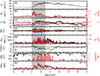 |
Figure 1 Solar wind, geomagnetic conditions, and FACs associated with a solar wind HSS during 19–26 March 2017. From top to bottom, the panels are: (a) solar wind proton speed Vp, (b) proton density Np (black, legend on the left) and ram pressure Psw (red, legend on the right), (c) proton temperature Tp (black, legend on the left) and plasma-β (red, legend on the right), (d) interplanetary magnetic field (IMF) magnitude B0, and Bx, By, and Bz components, (e) the Newell coupling function NCF (black, legend on the left) and dayside magnetic reconnection rate ΦD (red, legend on the right), (f) symmetric ring current index SYM-H, (g) westward auroral electrojet index SML (black, legend on the left) and number of substorm in each 3-h interval (red, legend on the right), and (h) total FAC intensity (FACT) in the northern hemisphere (NH; black) and southern hemisphere (SH; red). Vertical shading indicates a CIR. |
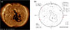 |
Figure 2 Coronal hole identified on 20 March 2017. (a) Solar image taken by NASA’s SDO/AIA telescope at the wavelength of 193 Å. The dark region around the center of the image is a coronal hole. (b) Solar synoptic map. The coronal hole is assigned NOAA number 72 and is characterized by a positive polarity magnetic field. |
The interaction region between the HSS and a slow stream with Vp of ~310–320 km s−1 (identified on 19–20 March) is characterized by enhanced peak Np (~53 cm–3, Fig. 1b), Psw (~15 nPa, Fig. 1b), and IMF B0 (~19 nT, Fig. 1d), representing plasma and magnetic field compressions inside a CIR.
The CIR and the HSS proper are characterized by enhanced magnetopause reconnection rate (ΦD, Fig. 1e) and consequent magnetic flux opening rate (NCF, Fig. 1e), leading to increases in the ring current (Fig. 1f) and auroral substorm activities (Fig. 1g) compared to the pre-CIR interval. While SML variation shows enhancement of substorm-related westward current intensity, the number of substorm occurrences in each 3-h interval substantially increased during the interval of high ΦD and NCF. However, the peak SYM-H is –46 nT, above the geomagnetic storm threshold (SYM-H ≤ –50 nT). This is consistent with the weaker geoeffectiveness of CIRs in causing geomagnetic storms (Tsurutani et al., 1995; see Tsurutani et al., 2024 for a discussion and an exception). Following the CIR onset, the total FAC intensities (FACT) increased to a peak of ~9 MA from a pre-CIR value of ~2 MA in both northern and southern hemispheres (Fig. 1h).
Figure 3 shows near-Earth solar wind conditions, geomagnetic and auroral responses, and FAC intensity variations from 1 June 2016 through 30 June 2017. Variation of Vp is characterized by multiple peaks (Fig. 3a). Analysis of individual peaks, associated plasma (Figs. 3a–3c), IMF parameters (Fig. 3d), and solar images (as described above) identifies thirty-three HSSs emanated from solar coronal holes. The HSS peak Vp values, their occurrence times, and magnetic polarities are listed in Table A1. We also identified two ICMEs during this interval. Descriptions of the ICMEs and associated FAC intensity variations are given in the Figures B1 and B2. The ICMEs are not included in the analyses that follow.
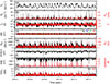 |
Figure 3 Solar wind, geomagnetic indices/conditions, and FAC intensities from 1 June 2016 through 30 June 2017. The panels are in the same format as in Figure 1. |
The HSS Vp peaks vary between ~486 and ~818 km s−1, with an average (median) Vp of ~704 ± 78 (~728) km s−1 for all HSSs (the number following the ± symbol is 1-σ deviation, which is only ~11% of the average Vp). Note that an HSS emanated from a polar coronal hole is assumed to have a peak Vp ~ 750–800 km s−1 (e.g., McComas et al., 2000). The lesser speeds recorded here are due to superradial expansion effects at the edges of the HSSs. The Vp peaks are preceded by peaks in Np (Fig. 3b), Psw (Fig. 3b), and IMF B0 (Fig. 3d), associated with plasma and IMF compressions in CIRs. All of the CIRs are associated with intensifications of the coupling functions NCF and ΦD (Fig. 3e), ring current index SYM-H (Fig. 3f), number of substorms and SML intensity (Fig. 3g), and FACT (Fig. 3h). These are consistent with the case study shown in Figure 1. Figure 3 clearly demonstrates the influence of repeating/periodic/recurring HSS impingements on the Earth’s magnetosphere-ionosphere system, as reflected in variations of the geomagnetic indices and currents.
Figure 4a shows Lomb-Scargle periodograms of the northern hemispheric FAC intensities (similar periodograms for solar wind parameters, coupling functions, auroral indices, and southern hemispheric FAC intensities are shown in Fig. C1). The FAC intensity periodograms are characterized by the strongest peak at ~13.8 days, followed by two weaker peaks at ~26.2 and ~29.2 days (both of the latter peaks are essentially at ~27 days). The periodicities are generally the same for dayside, nightside, and total FAC intensities in both the northern and southern hemispheres.
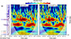 |
Figure 4 Periodogram analyses of FAC intensity and solar wind coupling. (a) Lomb-Scargle periodograms of the northern hemispheric total (black), dayside (red), and nightside (blue) FAC intensities; T represents total, D is dayside, N is nightside, NH is the northern hemisphere; and 95% confidence levels of the three periodograms are shown by three vertical lines. Cross-wavelet transforms of (b) northern hemispheric total FAC intensity and Vp, and (c) northern hemispheric total FAC intensity and NCF. Wavelet powers are shown by the color bar at the top. The cone of influence, where edge effects might distort the results, is shown in lighter shades. The relative phase relationships (of FAC intensity with Vp and NCF) are shown as arrows, horizontal right arrows indicating in-phase, horizontal left arrows indicating anti-phase. For the Lomb-Scargle periodograms, 2-min resolution FAC intensities are used, while for cross-wavelets, all data are processed into 30-min resolution (by taking 30-min running averages) so that they precisely coincide (in time) with each other. |
Figures 4b and 4c show cross-wavelets of total northern hemispheric FAC intensity with Vp and NCF, respectively. Phase differences of FAC intensity with Vp and NCF are indicated by the arrows, rightward-pointing (leftward-pointing) horizontal arrows indicating the in-phase (anti-phase) relationship. Based on the spectral power, the strongest common period for FAC intensity and Vp, as well as for FAC intensity and NCF, is centered around 28 days, followed by another peak at ~14 days. Both peaks have “intermittent” distributions. While the ~28-day period is observed from around 18 June 2016 through 27 November 2016 (~2016.47–2016.91) and from around 23 December 2016 through 7 June 2017 (~2016.98–2017.43), the ~14-day period is most prominent from around 4 August 2016 through 7 March 2017 (~2016.59–2017.18). The existence of common periodicities between FAC intensity and Vp, and between FAC intensity and NCF, is indicative of the close relationships of FAC intensity with Vp and NCF.
The phase relationship of FAC intensities with Vp is different from that with NCF. While FAC intensities are mostly in-phase with Vp around the 28-day periodicity, phase differences between the two are prominent at a ~14-day period (Fig. 4b). On the contrary, FAC intensities are almost in-phase with NCF at both ~28 and ~14-day periodicities (Fig. 4c). However, slight differences in phase (between FAC intensity and NCF) are indicated by slightly downward-pointing arrows. This slightly out-of-phase relationship is consistent with a certain (~40–60 min) delay between the solar wind driving and the FAC intensity, as reported before (e.g., Pedersen et al., 2023). The minutes-to-hour scale time lags are not further explored as we are interested in longer scale trends in FACs. In addition, FAC intensity exhibits enhanced wavelet coherence with Vp around the ~28 and ~14-day periodicities, and with NCF for almost all periods (see Fig. C2).
Relationships of FAC intensities with solar wind plasma, IMF, and solar wind-magnetosphere coupling functions are further explored in Figure 5. They show variations of daily mean total FAC intensity (FACT), dayside FAC intensity (FACD) and nightside FAC intensity (FACN) in the northern (NH) and southern (SH) hemispheres with daily mean solar wind parameters and coupling functions (daily mean values are used as we are interested in long-term trends in FAC variations). All panels show linearly increasing trends in FACT, FACD, and FACN with increasing solar wind parameters and coupling functions. Pearson’s correlation coefficients obtained from the linear regression analysis are mentioned in each panel.
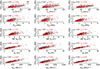 |
Figure 5 Variations of FAC intensities FACT (left column), FACD (middle column), and FACN (right column) with solar wind plasma, IMF, and solar wind-magnetosphere coupling functions Vp, Psw, IMF B0, ΦD, and NCF (from top to bottom panels). In each panel, black and red data correspond to the northern (NH) and southern (SH) hemispheric FACs, respectively. Pearson’s linear correlation coefficients (r) obtained from linear regression analyses are mentioned in each panel. The statistical significance of the correlation coefficients is confirmed by the Student’s t-test (Student. 1908). |
While correlations with FACs are weaker for Vp, Psw, IMF B0 (r = 0.48–0.66), stronger correlations are noted with the coupling functions ΦD (r = 0.82–0.92) and NCF (r = 0.79–0.90). FACN exhibits a stronger correlation than FACD, and correlations are slightly stronger for southern hemispheric FACs than for northern hemispheric FACs.
4 Discussion
We have presented the first observations of periodic variations of FAC intensities in response to recurrent solar wind HSSs during a solar cycle minimum condition. Both dayside and nightside FAC intensities in both the northern and southern hemispheres are characterized by distinct periodicities of ~14, ~26, and ~29 days.
It may be worth noting that Hajra et al. (2025a) reported ~19 and ~11 h periodicities in FAC intensities during HILDCAAs lasting for a few days to a week. The periodicities were attributed to interplanetary Alfvén waves (Korth et al., 2011; Tsurutani et al., 2006a). On the other hand, Hajra et al. (2025c) identified a ~1-year periodicity in solar cycle variation of FACs, which is not plausible to be driven by solar winds.
The solar activity minimum period is characterized by low solar ionizing fluxes (thus low ionospheric conductance) as well as low occurrences of solar transient activity such as solar flares and ICMEs (thus low occurrence of strong magnetospheric convection). However, cross-wavelet and coherence analyses confirmed causal relationships of FAC intensity variations with solar wind speed and solar wind-magnetosphere coupling. They are found to exhibit common periodicities centered around 14 and 27 days. The ~26 and ~29-day periodicities in FACs are close to the ~27-day solar rotation period, and we assume that they are essentially the same peak. The ~14-day FAC periodicity represents the first harmonic of the solar rotation period (Gosling et al., 1976; Zirker 1977; Lindblad & Lundstedt, 1981). The appearance of well-separated spectral peaks at ~26 and ~29 days may suggest an amplitude modulation of the FAC intensity, varying with the solar rotation period.
Modulation of FAC intensities by solar wind HSSs is statistically confirmed by significant linear correlations of both dayside and nightside FAC intensities with solar wind/interplanetary parameters and coupling functions. Correlations of FACs with solar wind-magnetosphere coupling functions are consistent with previous studies of FACs, but during auroral substorms (e.g., Coxon et al., 2014a), geomagnetic storms (e.g., Pedersen et al., 2023), and HILDCAAs (Hajra et al., 2025a). HSSs convect interplanetary Alfvén waves, the southward component of which causes magnetic reconnection at the dayside magnetopause (Dungey 1961). HSSs can also cause viscous interaction at the dayside magnetopause (Axford & Hines, 1961). Both of these processes are believed to lead to substorm activity. Clearly, the nightside FACs are associated with substorms (Coxon et al., 2014a, 2014b; Pedersen et al., 2021, 2022; Zhong et al., 2022; Wang et al., 2024; Hajra et al., 2025c).
However, it is possible that the dayside FACs are separate and distinct from the nightside substorm FAC events. Previous studies have revealed that dayside FAC intensities are controlled by ionospheric conductance (Fujii et al., 1981; Wang et al., 2005; Coxon et al., 2016; Hajra et al., 2025c). However, Tsurutani et al. (2001) showed that the dayside and nightside polar cap boundary layer waves were continuously connected in a 24-h local time oval. While ionospheric conductance varies with seasons due to solar irradiance variations, our results suggest that dayside FACs are also associated with either magnetic reconnection, viscous interaction, or both. This is consistent with recent studies (Zhong et al., 2022; Wang & Lühr, 2023; Wang et al., 2024) indicating that energetic particle precipitation may enhance the auroral ionospheric Hall conductance.
As expected, the FAC intensity exhibits better correlation with the coupling functions (ΦD and NCF) than with solar wind plasma and IMF parameters (Vp, Psw, IMF B0). In addition, FAC intensity exhibits better phase relationship with NCF than with Vp at the ~14-day periodicity. These results may be related to the fact that the higher values of NCF and FAC intensity are observed during the compression regions (CIRs) rather than during the HSSs. In other words, the physical driver of the FAC intensity modulation appears to be NCF, signifying enhanced solar wind-magnetosphere coupling in CIRs. Lower correlation with solar wind/IMF parameters (and higher correlation with coupling functions) may indicate combined roles of the plasma/IMF characteristic parameters in controlling geophysical processes.
5 Final comment
This study interval, June 2016 to June 2017, occurred during the solar activity minimum between solar cycles 24 and 25. It is noted that the interval was dominated by periodic (~27-day) solar wind HSSs which reached peak speeds of ~820 km s−1. In a previous work, Tsurutani et al. (2011) studied the solar wind and geomagnetic activity during the two previous solar minima between solar cycles 22 and 23, and between solar cycles 23 and 24. Due to the solar location of coronal holes during the previous two solar minima, the solar wind HSSs never approached their maximum speeds of ~820 km s−1 as shown in this 2016–2017 solar minimum. The two previous extreme minima in geomagnetic activity essentially established a ground state of the magnetosphere. We suggest that future studies of extreme solar minima be performed, which may allow resolution of some of the uncertainties in the physical causes of dayside and nightside FACs indicated in this paper.
Acknowledgments
We would like to acknowledge Aslak Grinsted for providing the wavelet coherence package used in this work, available at http://noc.ac.uk/using-science/crosswavelet-wavelet-coherence. We would like to thank the editors and reviewers for sharing extremely valuable suggestions, which substantially improved the manuscript. The editor thanks Hermann Lühr and an anonymous reviewer for their assistance in evaluating this paper.s
Funding
The work of RH is funded by the “Hundred Talents Program” of the Chinese Academy of Sciences (CAS), the “Excellent Young Scientists Fund Program (Overseas)”, and the “Research Fund for International Excellent Young Scientists” (grant number: W2532030) of the National Natural Science Foundation of China (NSFC). AMSF would like to thank the Institute of Geosciences and Engineering-UNIFESSPA (project n°. 23479.009478/2024-60). EE would like to thank the Brazilian agency CNPq for research grants (contract PQ-301883/2019-0 and PQ-303900-2024-5).
Conflict of interests
The authors declare no financial and non-financial competing interests.
Data availability statement
The FAC data are obtained from the AMPERE Science Data Center of the Johns Hopkins Applied Physics Laboratory (https://ampere.jhuapl.edu/). The data is available for free download from the AMPERE Derived Product Data Files (Daily) page (https://ampere.jhuapl.edu/download/?page=derivedProductsTab). The near-Earth solar wind plasma and IMF data are obtained from NASA’s OMNIWeb Plus database (https://omniweb.gsfc.nasa.gov/). The high-resolution data can be downloaded directly from the page: https://omniweb.gsfc.nasa.gov/form/omni_min.html, by specifying start and stop times. The solar SDO/AIA images are obtained from https://sdo.gsfc.nasa.gov/, and the NOAA solar synoptic maps are obtained from http://www.swpc.noaa.gov/. Geomagnetic SYM-H indices are obtained from the World Data Center for Geomagnetism, Kyoto, Japan (http://wdc.kugi.kyoto-u.ac.jp/). The indices can be freely downloaded from the “Plot and data output of ASY/SYM and AE indices” (https://wdc.kugi.kyoto-u.ac.jp/aeasy/index.html) by specifying start time and duration. The SML indices are obtained from the SuperMAG website (https://supermag.jhuapl.edu/). They can be freely downloaded from the Indices (https://supermag.jhuapl.edu/indices/) by specifying the index, time, and duration. The SuperMAG substorm list is collected from the Products (https://supermag.jhuapl.edu/products/?tab=download) by specifying the start and end times, and Substorm List as “Ohtani & Gjerloev, 2020”.
Author contribution statement
Conceptualization: RH, BTT; Methodology: RH; Validation: RH, BTT; Formal analysis: RH, AMSF; Investigation: RH, BTT; Resources: RH; Data Curation: RH; Visualization: RH; Supervision: RH, BTT; Funding acquisition: RH. Writing – Original Draft: RH; Writing – Review & Editing: RH, BTT, AMSF, QL, AD, GSL, SL, XG, EE. All authors read and approved the final manuscript.
References
- Alves, MV, Echer E, Gonzalez WD. 2006. Geoeffectiveness of corotating interaction regions as measured by Dst index. J. Geophys. Res. Space Physics 111: 2005JA011379. https://doi.org/10.1029/2005JA011379. [Google Scholar]
- Anderson, BJ, Takahashi K, Kamei T, Waters CL, Toth BA. 2002. Birkeland current system key parameters derived from Iridium observations: Method and initial validation results. J. Geophys. Res. Space Physics 107: SMP 11-1-SMP 11-13. https://doi.org/10.1029/2001JA000080. [Google Scholar]
- Araki, T, Funato K, Iguchi T, Kamei T. 1993. Direct detection of solar wind dynamic pressure effect on ground geomagnetic field. Geophys. Res. Lett. 20: 775–778. https://doi.org/10.1029/93GL00852. [Google Scholar]
- Axford, WI, Hines CO. 1961. A unifying theory of high-latitude geophyaical phenomena and geomagnetic storms. Can. J. Phys. 39: 1433–1464. https://doi.org/10.1139/p61-172. [Google Scholar]
- Baker, KB, Wing S. 1989. A new magnetic coordinate system for conjugate studies at high latitudes. J. Geophys. Res. 94: 9139–9143. https://doi.org/10.1029/JA094iA07p09139. [Google Scholar]
- Belcher, JW, Davis L. 1971. Large-amplitude Alfvén waves in the interplanetary medium, 2. J. Geophys. Res. 76: 3534–3563. https://doi.org/10.1029/JA076i016p03534. [NASA ADS] [CrossRef] [Google Scholar]
- Birkeland, K. 1908. The Norwegian Aurora Polaris Expedition, 1902-1903 (Vol. 1). H. Aschelhoug, Christiania. https://doi.org/10.5962/bhl.title.17857. [Google Scholar]
- Burlaga, LF, Sittler E, Mariani F, Schwenn R. 1981. Magnetic loop behind an interplanetary shock: Voyager, Helios, and IMP 8 observations. J. Geophys. Res. Space Physics 86: 6673–6684. https://doi.org/10.1029/JA086iA08p06673. [Google Scholar]
- Chi, Y, Shen C, Luo B, Wang Y, Xu M. 2018. Geoeffectiveness of Stream Interaction Regions From 1995 to 2016. Space Weather 16: 1960–1971. https://doi.org/10.1029/2018SW001894. [NASA ADS] [CrossRef] [Google Scholar]
- Coleman, PJ. 1966. Hydromagnetic Waves in the Interplanetary Plasma. Phys. Rev. Lett. 17: 207–211. https://doi.org/10.1103/PhysRevLett.17.207. [Google Scholar]
- Coxon, JC, Milan SE, Clausen LBN, Anderson BJ, Korth H. 2014a. A superposed epoch analysis of the regions 1 and 2 Birkeland currents observed by AMPERE during substorms. J. Geophys. Res. Space Physics 119: 9834–9846. https://doi.org/10.1002/2014JA020500. [Google Scholar]
- Coxon, JC, Milan SE, Clausen LBN, Anderson BJ, Korth H. 2014b. The magnitudes of the regions 1 and 2 Birkeland currents observed by AMPERE and their role in solar wind-magnetosphere-ionosphere coupling. J. Geophys. Res. Space Physics 119: 9804–9815. https://doi.org/10.1002/2014JA020138. [Google Scholar]
- Coxon, JC, Milan SE, Carter JA, Clausen LBN, Anderson BJ, et al. 2016. Seasonal and diurnal variations in AMPERE observations of the Birkeland currents compared to modeled results. J. Geophys. Res. Space Physics 121: 4027–4040. https://doi.org/10.1002/2015JA022050. [Google Scholar]
- Dessler, AJ, Parker EN. 1959. Hydromagnetic theory of geomagnetic storms. J. Geophys. Res. 64: 2239–2252. https://doi.org/10.1029/JZ064i012p02239. [Google Scholar]
- Dungey, JW. 1961. Interplanetary Magnetic Field and the Auroral Zones. Phys. Rev. Lett. 6: 47–48. https://doi.org/10.1103/PhysRevLett.6.47. [NASA ADS] [CrossRef] [Google Scholar]
- Fujii, R, Iijima T, Potemra TA, Sugiura M. 1981. Seasonal dependence of large-scale Birkeland currents. Geophys. Res. Lett. 8: 1103–1106. https://doi.org/10.1029/GL008i010p01103. [Google Scholar]
- Gjerloev, JW. 2009. A global ground-based magnetometer initiative. EOS Trans. Am. Geophys. Union 90: 230–231. https://doi.org/10.1029/2009EO270002. [Google Scholar]
- Gonzalez, WD, Tsurutani BT. 1987. Criteria of interplanetary parameters causing intense magnetic storms (Dst < −100 nT). Planet Space Sci 35: 1101–1109. https://doi.org/10.1016/0032-0633(87)90015-8. [Google Scholar]
- Gonzalez, WD, Joselyn JA, Kamide Y, Kroehl HW, Rostoker G, et al. 1994. What is a geomagnetic storm? J. Geophys. Res. Space Physics 99: 5771–5792. https://doi.org/10.1029/93JA02867. [Google Scholar]
- Gosling, JT, Asbridge JR, Bame SJ, Feldman WC. 1976. Solar wind speed variations: 1962-1974. J. Geophys. Res. 81: 5061–5070. https://doi.org/10.1029/JA081i028p05061. [Google Scholar]
- Grinsted, A, Moore JC, Jevrejeva S. 2004. Application of the cross wavelet transform and wavelet coherence to geophysical time series. Nonlinear Process. Geophys. 11: 561–566. https://doi.org/10.5194/npg-11-561-2004. [CrossRef] [Google Scholar]
- Hajra, R. 2021. Seasonal dependence of the Earth’s radiation belt – new insights. Ann. Geophys. 39: 181–187. https://doi.org/10.5194/angeo-39-181-2021. [Google Scholar]
- Hajra, R, Tsurutani BT. 2018. Magnetospheric “Killer” Relativistic Electron Dropouts (REDs) and Repopulation: A Cyclical Process. In Extreme Events in Geospace (pp. 373–400). Elsevier. https://doi.org/10.1016/B978-0-12-812700-1.00014-5. [Google Scholar]
- Hajra, R, Echer E, Tsurutani BT, Gonzalez WD. 2013. Solar cycle dependence of High-Intensity Long-Duration Continuous AE Activity (HILDCAA) events, relativistic electron predictors? J. Geophys. Res. Space Physics 118: 5626–5638. https://doi.org/10.1002/jgra.50530. [Google Scholar]
- Hajra, R, Tsurutani BT, Echer E, Gonzalez WD. 2014a. Relativistic electron acceleration during high-intensity, long-duration, continuous AE activity (HILDCAA) events: Solar cycle phase dependences: Relativistic electrons during HILDCAAs. Geophys. Res. Lett. 41: 1876–1881. https://doi.org/10.1002/2014GL059383. [Google Scholar]
- Hajra, R, Echer E, Tsurutani BT, Gonzalez WD. 2014b. Superposed epoch analyses of HILDCAAs and their interplanetary drivers: Solar cycle and seasonal dependences. J Atmos Sol Terr Phys 121: 24–31. https://doi.org/10.1016/j.jastp.2014.09.012. [Google Scholar]
- Hajra, R, Tsurutani BT, Echer E, Gonzalez WD, Santolik O. 2015a. Relativistic (E > 0.6, > 2.0, and > 4.0 MeV) electron acceleration at geosynchronous orbit during high-intensity, long-duration, continuous AE activity (HILDCAA) events. Astrophys. J. 799: 39. https://doi.org/10.1088/0004-637X/799/1/39. [Google Scholar]
- Hajra, R, Tsurutani BT, Echer E, Gonzalez WD, Brum CGM, et al. 2015b. Relativistic electron acceleration during HILDCAA events: are precursor CIR magnetic storms important? Earth Planet Space 67: 109. https://doi.org/10.1186/s40623-015-0280-5. [Google Scholar]
- Hajra, R, Franco AMS, Echer E, Bolzan MJA. 2021. Long-term variations of the geomagnetic activity: a comparison between the strong and weak solar activity cycles and implications for the space climate. J. Geophys. Res. Space Physics 126: e2020JA028695. https://doi.org/10.1029/2020JA028695. [Google Scholar]
- Hajra, R, Echer E, Franco AMS, Bolzan MJA. 2023. Earth’s magnetotail variability during supersubstorms (SSSs): A study on solar wind–magnetosphere–ionosphere coupling. Adv. Space Res. 72: 1208–1223. https://doi.org/10.1016/j.asr.2023.04.013. [Google Scholar]
- Hajra, R, Tsurutani BT, Lakhina GS, Lu Q, Du A. 2024a. Interplanetary Causes and Impacts of the 2024 May Superstorm on the Geosphere: An Overview. Astrophys. J. 974: 264. https://doi.org/10.3847/1538-4357/ad7462. [Google Scholar]
- Hajra, R, Tsurutani BT, Lu Q, Horne RB, Lakhina GS, et al. 2024b. The April 2023 SYM-H = −233 nT Geomagnetic Storm: A Classical Event. J. Geophys. Res. Space Physics 129: e2024JA032986. https://doi.org/10.1029/2024JA032986. [Google Scholar]
- Hajra, R, Tsurutani BT, Lu Q, Lakhina GS., Du A, et al. 2024c. Ultra-relativistic Electron Acceleration during High-intensity Long-duration Continuous Auroral Electrojet Activity Events. Astrophys. J. 965: 146. https://doi.org/10.3847/1538-4357/ad2dfe. [Google Scholar]
- Hajra, R, Tsurutani BT, Lu Q, Du A, Lu S, et al. 2025a. Field-Aligned Currents during High-Intensity Long-Duration Continuous Auroral Electrojet Activity Events: A Statistical Study. Space Weather 23: e2025SW004353. https://doi.org/10.1029/2025SW004353. [Google Scholar]
- Hajra, R, Tsurutani BT, Lu Q, Du A. 2025b. Field-Aligned Currents during High-Intensity Long-Duration Continuous Auroral Electrojet Activity Events: Seasonal Dependences. Space Weather 23: e2025SW004354. https://doi.org/10.1029/2025SW004354. [Google Scholar]
- Hajra, R, Tsurutani BT, Lu Q, Du A, Lu S, et al. 2025c. Solar cycle and seasonal dependences of field-aligned currents. Space Weather 23: e2025SW004441. https://doi.org/10.1029/2025SW004441. [Google Scholar]
- Iijima, T, Potemra TA. 1976. The amplitude distribution of field-aligned currents at northern high latitudes observed by Triad. J. Geophys. Res. 81: 2165–2174. https://doi.org/10.1029/JA081i013p02165. [Google Scholar]
- Iijima, T, Potemra TA. 1978. Large-scale characteristics of field-aligned currents associated with substorms. J. Geophys. Res. Space Physics 83: 599–615. https://doi.org/10.1029/JA083iA02p00599. [Google Scholar]
- Iyemori, T. 1990. Storm-time magnetospheric currents inferred from mid-latitude geomagnetic field variations. J. Geomagn. Geoelectr. 42: 1249–1265. https://doi.org/10.5636/jgg.42.1249. [Google Scholar]
- Kennel, CF, Edmiston JP, Hada T. 1985. A Quarter Century of Collisionless Shock Research. In RG Stone, BT Tsurutani (Eds.), Geophys Mono Ser, Am Geophys Union, Washington, D.C., pp. 1–36. https://doi.org/10.1029/GM034p0001. [Google Scholar]
- King, JH, Papitashvili NE. 2020. OMNI 1-min Data Set [Data set]. NASA Space Physics Data Facility. https://doi.org/10.48322/45BB-8792. [Google Scholar]
- Knipp, DJ, Matsuo T, Kilcommons L, Richmond A, Anderson B, et al. 2014. Comparison of magnetic perturbation data from LEO satellite constellations: Statistics of DMSP and AMPERE. Space Weather 12: 2–23. https://doi.org/10.1002/2013SW000987. [Google Scholar]
- Korth, A, Echer E, Zong QG, Guarnieri FL, Fraenz M, et al. 2011. The response of the polar cusp to a high-speed solar wind stream studied by a multispacecraft wavelet analysis. J Atmos Sol Terr Phys 73: 52–60. https://doi.org/10.1016/j.jastp.2009.10.004. [Google Scholar]
- Krieger, AS, Timothy AF, Roelof EC. 1973. A coronal hole and its identification as the source of a high velocity solar wind stream. Sol. Phys. 29: 505–525. https://doi.org/10.1007/BF00150828. [NASA ADS] [CrossRef] [Google Scholar]
- Lakhina, GS, Tsurutani BT, Kojima H, Matsumoto H. 2000. “Broadband” plasma waves in the boundary layers. J. Geophys. Res. Space Physics 105: 27791–27831. https://doi.org/10.1029/2000JA900054. [Google Scholar]
- Lakhina, GS, Tsurutani BT, Singh SV, Reddy RV. 2003. Some theoretical models for solitary structures of boundary layer waves. Nonlinear Process. Geophys. 10: 65–73. https://doi.org/10.5194/npg-10-65-2003. [Google Scholar]
- Le, G, Lühr H, Anderson BJ, Strangeway RJ, Russell CT, et al. 2016. Magnetopause erosion during the 17 March 2015 magnetic storm: Combined field-aligned currents, auroral oval, and magnetopause observations. Geophys. Res. Lett. 43: 2396–2404https://doi.org/10.1002/2016GL068257. [NASA ADS] [CrossRef] [Google Scholar]
- Lindblad, BA, Lundstedt H. 1981. A catalogue of high-speed plasma streams in the solar wind. Sol. Phys. 74: 197–206. https://doi.org/10.1007/BF00151290. [Google Scholar]
- Lomb, NR. 1976. Least-squares frequency analysis of unequally spaced data. Astrophys Space Sci 39: 447–462. https://doi.org/10.1007/BF00648343. [CrossRef] [Google Scholar]
- Lyons, LR, Gallardo Lacourt B, Zou S, Weygand JM, Nishimura Y, et al. 2016. The 17 March 2013 storm: Synergy of observations related to electric field modes and their ionospheric and magnetospheric Effects. J. Geophys. Res. Space Physics 121: 10880–10897. https://doi.org/10.1002/2016JA023237. [Google Scholar]
- Marubashi, K, Lepping RP. 2007. Long-duration magnetic clouds: a comparison of analyses using torus- and cylinder-shaped flux rope models. Ann. Geophys. 25: 2453–2477. https://doi.org/10.5194/angeo-25-2453-2007. [Google Scholar]
- McComas, DJ, Barraclough BL, Funsten HO, Gosling JT, Santiago Muñoz E, et al. 2000. Solar wind observations over Ulysses’ first full polar orbit. J. Geophys. Res. Space Physics 105: 10419–10433. https://doi.org/10.1029/1999JA000383. [Google Scholar]
- Milan, SE, Gosling JS, Hubert B. 2012. Relationship between interplanetary parameters and the magnetopause reconnection rate quantified from observations of the expanding polar cap. J. Geophys. Res. Space Physics 117: 2011JA017082. https://doi.org/10.1029/2011JA017082. [Google Scholar]
- Neugebauer, M, Clay DR, Goldstein BE, Tsurutani BT, Zwickl RD. 1984. A reexamination of rotational and tangential discontinuities in the solar wind. J. Geophys. Res. Space Physics 89: 5395–5408. https://doi.org/10.1029/JA089iA07p05395. [Google Scholar]
- Newell, PT, Sotirelis T, Liou K, Meng CI, Rich FJ. 2007. A nearly universal solar wind-magnetosphere coupling function inferred from 10 magnetospheric state variables. J. Geophys. Res. Space Physics 112: 2006JA012015. https://doi.org/10.1029/2006JA012015. [Google Scholar]
- Ohtani, S, Gjerloev JW. 2020. Is the Substorm Current Wedge an Ensemble of Wedgelets?: Revisit to Midlatitude Positive Bays. J. Geophys. Res. Space Physics 125: e2020JA027902. https://doi.org/10.1029/2020JA027902. [Google Scholar]
- Paulikas, GA, Blake JB. 1979. Effects of the Solar Wind on Magnetospheric Dynamics: Energetic Electrons at the Synchronous Orbit. In WP Olson (Ed.), Geophys Mono Ser, Am Geophys Union, Washington, D. C., pp. 180–202. https://doi.org/10.1029/GM021p0180. [Google Scholar]
- Pedersen, MN, Vanhamäki H, Aikio AT, Käki S, Workayehu AB, et al. 2021. Field-aligned and ionospheric currents by AMPERE and SuperMAG during HSS/SIR-driven storms. J. Geophys. Res. Space Physics 126: e2021JA029437. https://doi.org/10.1029/2021JA029437. [Google Scholar]
- Pedersen, MN, Vanhamäki H, Aikio AT, Waters CL, Gjerloev JW, et al. 2022. Effect of ICME-Driven Storms on Field-Aligned and Ionospheric Currents From AMPERE and SuperMAG. J. Geophys. Res. Space Physics 127: e2022JA030423. https://doi.org/10.1029/2022JA030423. [Google Scholar]
- Pedersen, MN, Vanhamäki H, Aikio AT. 2023. Comparison of field-aligned current responses to HSS/SIR, sheath, and magnetic cloud driven geomagnetic storms. Geophys. Res. Lett. 50: e2023GL103151. https://doi.org/10.1029/2023GL103151. [Google Scholar]
- Scargle, JD. 1982. Studies in astronomical time series analysis. II - Statistical aspects of spectral analysis of unevenly spaced data. Astrophys. J. 263: 835. https://doi.org/10.1086/160554. [Google Scholar]
- Sckopke, N. 1966. A general relation between the energy of trapped particles and the disturbance field near the Earth. J. Geophys. Res. 71: 3125–3130. https://doi.org/10.1029/JZ071i013p03125. [Google Scholar]
- Smith, EJ, Wolfe JH. 1976. Observations of interaction regions and corotating shocks between one and five AU: Pioneers 10 and 11. Geophys. Res. Lett. 3: 137–140. https://doi.org/10.1029/GL003i003p00137. [Google Scholar]
- Souza, AM, Echer E, Bolzan MJA, Hajra R. 2016. A study on the main periodicities in interplanetary magnetic field Bz component and geomagnetic AE index during HILDCAA events using wavelet analysis. J Atmos Sol Terr Phys 149: 81–86. https://doi.org/10.1016/j.jastp.2016.09.006. [Google Scholar]
- Souza, AM, Echer E, Bolzan MJA, Hajra R. 2018. Cross-correlation and cross-wavelet analyses of the solar wind IMF Bz and auroral electrojet index AE coupling during HILDCAAs. Ann. Geophys. 36: 205–211. https://doi.org/10.5194/angeo-36-205-2018. [CrossRef] [Google Scholar]
- Student. 1908. The Probable Error of a Mean. Biometrika 6: 1. https://doi.org/10.2307/2331554. [CrossRef] [Google Scholar]
- Tanskanen, EI, Slavin JA, Tanskanen AJ, Viljanen A, Pulkkinen TI, et al. 2005. Magnetospheric substorms are strongly modulated by interplanetary high-speed streams. Geophys. Res. Lett. 32: 2005GL023318. https://doi.org/10.1029/2005GL023318. [Google Scholar]
- Tsurutani, BT, Gonzalez WD. 1987. The cause of high-intensity long-duration continuous AE activity (HILDCAAs): Interplanetary Alfvén wave trains. Planet Space Sci 35: 405–412. https://doi.org/10.1016/0032-0633(87)90097-3. [Google Scholar]
- Tsurutani, BT, Lakhina GS. 2014. An extreme coronal mass ejection and consequences for the magnetosphere and Earth. Geophys. Res. Lett. 41: 287–292https://doi.org/10.1002/2013GL058825. [NASA ADS] [CrossRef] [Google Scholar]
- Tsurutani, BT, Gonzalez WD, Tang F, Akasofu SI, Smith EJ. 1988. Origin of interplanetary southward magnetic fields responsible for major magnetic storms near solar maximum (1978–1979). J. Geophys. Res. Space Physics 93: 8519–8531. https://doi.org/10.1029/JA093iA08p08519. [Google Scholar]
- Tsurutani, BT, Gonzalez WD, Gonzalez ALC, Tang F, Arballo JK, et al. 1995. Interplanetary origin of geomagnetic activity in the declining phase of the solar cycle. J. Geophys. Res. Space Physics 100: 21717–21733. https://doi.org/10.1029/95JA01476. [Google Scholar]
- Tsurutani, BT, Lakhina GS, Ho CM, Arballo, JK, Galvan C, et al. 1998. Broadband plasma waves observed in the polar cap boundary layer: Polar. J. Geophys. Res. Space Physics 103: 17351–17366. https://doi.org/10.1029/97JA03063. [Google Scholar]
- Tsurutani, BT, Zhou XY, Vasyliunas VM, Haerendel G, Arballo JK, et al. 2001. Interplanetary Shocks, Magnetopause Boundary Layers and Dayside Auroras: The Importance of a Very Small Magnetospheric Region. Surv. Geophys. 22: 101–130. https://doi.org/10.1023/A:1012952414384. [Google Scholar]
- Tsurutani, BT, Gonzalez WD, Gonzalez ALC, Guarnieri FL, Gopalswamy N, et al. 2006a. Corotating solar wind streams and recurrent geomagnetic activity: A review. J. Geophys. Res. 111: A07S01. https://doi.org/10.1029/2005JA011273. [Google Scholar]
- Tsurutani, BT, McPherron RL, Gonzalez WD, Lu G, Gopalswamy N, et al. 2006b. Magnetic storms caused by corotating solar wind streams. In BT Tsurutani, R McPherron, W Gonzalez, G Lu, JHA Sobral, N Gopalswamy (Eds.), Geophys Mono Ser (Vol. 167, pp. 1–17). Washington, D. C.: Am Geophys Union. https://doi.org/10.1029/167GM03. [Google Scholar]
- Tsurutani, BT, Echer E, Gonzalez WD. 2011. The solar and interplanetary causes of the recent minimum in geomagnetic activity (MGA23): a combination of midlatitude small coronal holes, low IMF BZ variances, low solar wind speeds and low solar magnetic fields. Ann. Geophys. 29, 839–849. https://doi.org/10.5194/angeo-29-839-2011. [Google Scholar]
- Tsurutani, BT, Lakhina GS, Verkhoglyadova OP, Gonzalez WD, Echer E, et al. 2011b. A review of interplanetary discontinuities and their geomagnetic effects. J Atmos Sol Terr Phys 73: 5–19. https://doi.org/10.1016/j.jastp.2010.04.001. [Google Scholar]
- Tsurutani, BT, Hajra R, Echer E, Gonzalez WD, Santolik O. 2016, June 1. Predicting Magnetospheric Relativistic >1 MeV Electrons (Version 40). Retrieved from http://www.techbriefs.com/component/content/article/ntb/tech-briefs/software/24815. [Google Scholar]
- Tsurutani, BT, Hajra R, Lakhina GS, Meng X. 2024. Revisiting the superstorm on 6–7 April 2000 caused by an extraordinary corotating interaction region (With an Embedded Coronal Jet?). J. Geophys. Res. Space Physics 129: e2024JA032989. https://doi.org/10.1029/2024JA032989. [Google Scholar]
- Wang, H, Lühr H. 2023. Magnetic longitudinal and local time variations of polar electrojet and field-aligned currents. J. Geophys. Res. Space Physics 128: e2023JA031874. https://doi.org/10.1029/2023JA031874. [Google Scholar]
- Wang, H, Lühr H, Ma SY. 2005. Solar zenith angle and merging electric field control of field-aligned currents: A statistical study of the Southern Hemisphere. J. Geophys. Res. Space Physics 110: 2004JA010530. https://doi.org/10.1029/2004JA010530. [Google Scholar]
- Wang, H, Lühr H, Ma SY, Weygand J, Skoug RM, et al. 2006. Field-aligned currents observed by CHAMP during the intense 2003 geomagnetic storm events. Ann. Geophys. 24: 311–324. https://doi.org/10.5194/angeo-24-311-2006. [Google Scholar]
- Wang, H, Cheng Q, Lühr H, Zhong Y, Zhang K, et al. 2024. Local time and hemispheric asymmetries of field-aligned currents and polar electrojet during May 2024 superstorm periods. J. Geophys. Res. Space Physics 129: e2024JA033020. https://doi.org/10.1029/2024JA033020. [Google Scholar]
- Waters, CL, Anderson BJ, Liou K. 2001. Estimation of global field aligned currents using the iridium® System magnetometer data. Geophys. Res. Lett. 28: 2165–2168. https://doi.org/10.1029/2000GL012725. [NASA ADS] [CrossRef] [Google Scholar]
- Wilder, FD, Crowley G, Anderson BJ, Richmond AD. 2012. Intense dayside Joule heating during the 5 April 2010 geomagnetic storm recovery phase observed by AMIE and AMPERE. J. Geophys. Res. Space Physics 117: 2011JA017262https://doi.org/10.1029/2011JA017262. [Google Scholar]
- Zhong, Y, Wang H, Zhang K, Xia H, Qian C. 2022. Local time response of auroral electrojet during magnetically disturbed periods: DMSP and CHAMP coordinated observations. J. Geophys. Res. Space Physics 127: e2022JA030624. https://doi.org/10.1029/2022JA030624. [Google Scholar]
- Zirker, JB. 1977. Coronal holes and high-speed wind streams. Rev. Geophys. 15: 257–269. https://doi.org/10.1029/RG015i003p00257. [NASA ADS] [CrossRef] [Google Scholar]
Cite this article as: Hajra R, Tsurutani BT, Franco AMS, Lu Q, Du A, et al.2026. Field-aligned currents are strongly modulated by corotating solar wind high-speed streams. J. Space Weather Space Clim. 16, 18. https://doi.org/10.1051/swsc/2026007
Appendix A: List of HSSs
HSSs under this study. Sunward (anti-sunward) HSSs are emanated from solar coronal holes with negative (positive) magnetic polarity, and are characterized by positive (negative) IMF Bx and negative (positive) By components.
Appendix B: ICMEs
Figure B1 shows an ICME and associated FAC variations during 19–23 July 2016. Sharp and simultaneous increases in the solar wind Vp (Fig. B1a), Np (Fig. B1b), Psw (Fig. B1b), Tp (Fig. B1c), and IMF B0 (Fig. B1d) at ~23:52 UT on 19 July represent a fast forward (FF) interplanetary shock (Kennel et al., 1985; Tsurutani et al., 2011b) (marked by a vertical dashed line, detail shock analysis is beyond scope of the present work) that caused a sudden impulse (SI+; Araki et al., 1993; Tsurutani et al., 2011b; Tsurutani & Lakhina, 2014) of +55 nT in SYM-H (Fig. B1f). The shock is caused by the interplanetary counterpart of a fast coronal mass ejection (CME), which was erupted from a solar active region at ~18:00 UT on 18 July. The shock compressed the plasma and IMF up to ~13:14 UT on 20 July, resulting in an interplanetary sheath (Kennel et al., 1985; Tsurutani et al., 1988). The sheath is followed by a region up to ~14:58 UT on 22 July (marked by a gray shading), where IMF components exhibit smooth rotations in polarities, Tp, and plasma-β (β being the ratio of the plasma pressure to the magnetic pressure) are low. This is called a magnetic cloud (MC; Burlaga et al., 1981; Gonzalez & Tsurutani, 1987; Marubashi & Lepping, 2007). While Bz had some small southward components in the sheath, it was weak, and the IMF was mainly northward during the MC. The shock triggered significant flux opening (high NCF) at the dayside magnetopause (Fig. B1e) during the sheath. As a consequence, there is some moderate substorm activity (Fig. B1g) and FAC enhancements (Fig. B1h) during the sheath. However, the MC is characterized by extremely low values of NCF and ΦD, no significant substorm activity, and no FAC enhancements.
The 12–20 October 2016 interval, shown in Figure B2, is characterized by an ICME followed by a solar wind HSS. The FF shock at ~22:12 UT on 12 October, marked by sharp increases in Vp (Fig. B2a), Np (Fig. B2b), Psw (Fig. B2b), Tp (Fig. B2c), and IMF B0 (Fig. B2d), is caused by the interplanetary counterpart of a fast CME erupted from the Sun at ~19:24 UT on 11 October. The shock led to an SI+ of +20 nT (Fig. B2f), followed by an interplanetary sheath of compressed plasma and fluctuating IMF up to ~06:09 UT on 13 October. The sheath is followed by an MC up to ~16:53 UT on 14 October (marked by a gray shading). It is characterized by a strong IMF B0, with clear and smooth rotations in its components, low Tp, and β. The strong IMF southward component Bz = –21 nT is associated with prominent increases in NCF (Fig. B2e), ΦD (Fig. B2e), strong substorm activity with peak SML = –2292 nT (Fig. B2g), an intense storm with SYM-H peak = –114 nT (Fig. B2f), and prominent FAC intensifications up to ~11 MA (Fig. B2h).
The MC is followed by a gradual rise in Vp to a peak value of ~750–777 km s−1 during 16–18 October, and then a slow decay in Vp (Fig. B2a). This is identified to be an HSS emanated from a negative polarity coronal hole on 14 October (not shown). The entire HSS proper was characterized by enhanced FACs of ~6 MA (Fig. B2h).
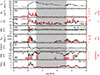 |
Figure B1. Solar wind, geomagnetic conditions, and FACs associated with an ICME during 19–23 July 2016. From top to bottom, the panels are: (a) solar wind Vp, (b) Np (black, legend on the left) and Psw (red, legend on the right), (c) Tp (black, legend on the left) and plasma-β (red, legend on the right), (d) IMF B0, and Bx, By, and Bz components, (e) NCF (black, legend on the left) and ΦD (red, legend on the right), (f) SYM-H index, (g) SML index (black, legend on the left) and substorm numbers in each 3-h interval (red, legend on the right), and (h) FACT in the northern hemisphere (NH; black) and southern hemisphere (SH; red). The dashed vertical line indicates an FF shock, and the shaded region is an MC. |
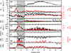 |
Figure B2. Solar wind, geomagnetic conditions, and FACs associated with an ICME followed by an HSS during 12–20 October 2016. Panels are the same as in Figure B1. The dashed vertical line indicates an FF shock, and the shaded region is an MC. |
Appendix C: Periodograms and wavelet coherence
Figure C1 shows Lomb-Scargle periodogram analyses of solar wind plasma, IMF, coupling functions, geomagnetic indices, and FAC intensities. Separate analyses are done for currents in the northern and southern hemispheres, and for dayside and nightside FACs.
The Vp periodogram is characterized by two prominent peaks: the strongest one at ~26 days, and a slightly weaker peak (~74% of the strongest peak) at ~13.6 days (Fig. C1a). For the plasma parameters Np, Psw, and Tp, the ~26 and 13.6-day periodicities have comparable amplitudes (Fig. C1b). In addition, Tp exhibits a prominent peak (~59%) at ~29 days, while Psw exhibits shorter periods of ~6.8 (~86%), ~4.5 (~71%), ~6.6 (~56%), 8.7 (~54%), and ~4.4 (~50%) days (in descending order of amplitude). IMF B0 exhibits the strongest peak at ~13.6 days, while Bz at ~25.3 days, with secondary peaks at ~14.1 (~87%) and multiple shorter (~2.7, 3.5, 2.5, 6.3, 4.2, 3.9 days) and longer (~25.4, 36.1, 29.3 days) periodicities (Fig. C1c).
ΦD and NCF are characterized by the strongest peak at ~13.8 days, followed by two peaks at ~26.1 (62–89%) and ~29.2 (68–76%) days (Fig. C1d). The ΦD and NCF periodicities are also present in the SML index (Fig. C1e), as well as in the FAC intensities (Figs. C1f–C1h). The strongest peak in FACs is noted at ~13.8 days, followed by peaks at ~26.2 and ~29.2 days. The periodicities are more or less the same for dayside, nightside, and total FACs in both the northern and southern hemispheres.
Figure C2 shows the wavelet coherences between the northern hemispheric total FAC intensity and Vp (Fig. C2a), and between FAC intensity and NCF (Fig. C2b), with the arrows representing the phase differences (as in Fig. 4). FAC intensity is strongly coherent to NCF for most of the periods. However, FAC exhibits lesser coherence with Vp for periods < 7 days, periods of ~18–20 days, and periods of ~39–56 days. In other words, FAC intensity is much more coherent to NCF than to Vp.
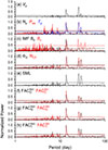 |
Figure C1. Lomb-Scargle periodograms of solar wind plasma and IMF parameters, solar wind-magnetosphere coupling functions, auroral electrojet indices, and FAC intensities. In panels (f)–(h), T represents total, D is dayside, N is nightside, NH is the northern hemisphere, and SH is the southern hemisphere. Horizontal lines in each panel indicate 95% confidence levels of the periodograms. For the periodogram analyses, we used the highest resolution data available, i.e., 2 min for FACs and 1 min for all other parameters. |
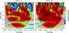 |
Figure C2. Wavelet coherence (a) between northern hemispheric total FAC intensity and Vp, and (b) between northern hemispheric total FAC intensity and NCF. Wavelet coherence values are shown by the color bar at the right. The cone of influence, where edge effects might distort the results, is shown as lighter shades. The relative phase relationships (of FAC intensity with Vp and NCF) are shown as arrows, horizontal right arrows indicating in-phase, horizontal left arrows indicating anti-phase. All data are processed into 30 min resolution so that they precisely coincide (in time) with each other. |
All Tables
HSSs under this study. Sunward (anti-sunward) HSSs are emanated from solar coronal holes with negative (positive) magnetic polarity, and are characterized by positive (negative) IMF Bx and negative (positive) By components.
All Figures
|
Figure 1 Solar wind, geomagnetic conditions, and FACs associated with a solar wind HSS during 19–26 March 2017. From top to bottom, the panels are: (a) solar wind proton speed Vp, (b) proton density Np (black, legend on the left) and ram pressure Psw (red, legend on the right), (c) proton temperature Tp (black, legend on the left) and plasma-β (red, legend on the right), (d) interplanetary magnetic field (IMF) magnitude B0, and Bx, By, and Bz components, (e) the Newell coupling function NCF (black, legend on the left) and dayside magnetic reconnection rate ΦD (red, legend on the right), (f) symmetric ring current index SYM-H, (g) westward auroral electrojet index SML (black, legend on the left) and number of substorm in each 3-h interval (red, legend on the right), and (h) total FAC intensity (FACT) in the northern hemisphere (NH; black) and southern hemisphere (SH; red). Vertical shading indicates a CIR. |
| In the text | |
|
Figure 2 Coronal hole identified on 20 March 2017. (a) Solar image taken by NASA’s SDO/AIA telescope at the wavelength of 193 Å. The dark region around the center of the image is a coronal hole. (b) Solar synoptic map. The coronal hole is assigned NOAA number 72 and is characterized by a positive polarity magnetic field. |
| In the text | |
|
Figure 3 Solar wind, geomagnetic indices/conditions, and FAC intensities from 1 June 2016 through 30 June 2017. The panels are in the same format as in Figure 1. |
| In the text | |
|
Figure 4 Periodogram analyses of FAC intensity and solar wind coupling. (a) Lomb-Scargle periodograms of the northern hemispheric total (black), dayside (red), and nightside (blue) FAC intensities; T represents total, D is dayside, N is nightside, NH is the northern hemisphere; and 95% confidence levels of the three periodograms are shown by three vertical lines. Cross-wavelet transforms of (b) northern hemispheric total FAC intensity and Vp, and (c) northern hemispheric total FAC intensity and NCF. Wavelet powers are shown by the color bar at the top. The cone of influence, where edge effects might distort the results, is shown in lighter shades. The relative phase relationships (of FAC intensity with Vp and NCF) are shown as arrows, horizontal right arrows indicating in-phase, horizontal left arrows indicating anti-phase. For the Lomb-Scargle periodograms, 2-min resolution FAC intensities are used, while for cross-wavelets, all data are processed into 30-min resolution (by taking 30-min running averages) so that they precisely coincide (in time) with each other. |
| In the text | |
|
Figure 5 Variations of FAC intensities FACT (left column), FACD (middle column), and FACN (right column) with solar wind plasma, IMF, and solar wind-magnetosphere coupling functions Vp, Psw, IMF B0, ΦD, and NCF (from top to bottom panels). In each panel, black and red data correspond to the northern (NH) and southern (SH) hemispheric FACs, respectively. Pearson’s linear correlation coefficients (r) obtained from linear regression analyses are mentioned in each panel. The statistical significance of the correlation coefficients is confirmed by the Student’s t-test (Student. 1908). |
| In the text | |
|
Figure B1. Solar wind, geomagnetic conditions, and FACs associated with an ICME during 19–23 July 2016. From top to bottom, the panels are: (a) solar wind Vp, (b) Np (black, legend on the left) and Psw (red, legend on the right), (c) Tp (black, legend on the left) and plasma-β (red, legend on the right), (d) IMF B0, and Bx, By, and Bz components, (e) NCF (black, legend on the left) and ΦD (red, legend on the right), (f) SYM-H index, (g) SML index (black, legend on the left) and substorm numbers in each 3-h interval (red, legend on the right), and (h) FACT in the northern hemisphere (NH; black) and southern hemisphere (SH; red). The dashed vertical line indicates an FF shock, and the shaded region is an MC. |
| In the text | |
|
Figure B2. Solar wind, geomagnetic conditions, and FACs associated with an ICME followed by an HSS during 12–20 October 2016. Panels are the same as in Figure B1. The dashed vertical line indicates an FF shock, and the shaded region is an MC. |
| In the text | |
|
Figure C1. Lomb-Scargle periodograms of solar wind plasma and IMF parameters, solar wind-magnetosphere coupling functions, auroral electrojet indices, and FAC intensities. In panels (f)–(h), T represents total, D is dayside, N is nightside, NH is the northern hemisphere, and SH is the southern hemisphere. Horizontal lines in each panel indicate 95% confidence levels of the periodograms. For the periodogram analyses, we used the highest resolution data available, i.e., 2 min for FACs and 1 min for all other parameters. |
| In the text | |
|
Figure C2. Wavelet coherence (a) between northern hemispheric total FAC intensity and Vp, and (b) between northern hemispheric total FAC intensity and NCF. Wavelet coherence values are shown by the color bar at the right. The cone of influence, where edge effects might distort the results, is shown as lighter shades. The relative phase relationships (of FAC intensity with Vp and NCF) are shown as arrows, horizontal right arrows indicating in-phase, horizontal left arrows indicating anti-phase. All data are processed into 30 min resolution so that they precisely coincide (in time) with each other. |
| In the text | |
Current usage metrics show cumulative count of Article Views (full-text article views including HTML views, PDF and ePub downloads, according to the available data) and Abstracts Views on Vision4Press platform.
Data correspond to usage on the plateform after 2015. The current usage metrics is available 48-96 hours after online publication and is updated daily on week days.
Initial download of the metrics may take a while.