| Issue |
J. Space Weather Space Clim.
Volume 10, 2020
|
|
|---|---|---|
| Article Number | 61 | |
| Number of page(s) | 24 | |
| DOI | https://doi.org/10.1051/swsc/2020062 | |
| Published online | 07 December 2020 | |
Research Article
Semi-annual, annual and Universal Time variations in the magnetosphere and in geomagnetic activity: 3. Modelling
1
Department of Meteorology, University of Reading, Reading, RG6 6BB, UK
2
School of Physics and Astronomy, University of Southampton, Southampton, SO17 1BJ, UK
3
Institute of Space and Atmospheric Studies, University of Saskatchewan, Saskatoon, Saskatchewan, S7N 5E2, Canada
* Corresponding author: This email address is being protected from spambots. You need JavaScript enabled to view it.
Received:
13
September
2020
Accepted:
11
October
2020
Abstract
This is the third in a series of papers that investigate the semi-annual, annual and Universal Time variations in the magnetosphere. In this paper, we use the Lin et al. (2010) empirical model of magnetopause locations, along with the assumption of pressure equilibrium and the Newtonian approximation of magnetosheath pressure, to show that the equinoctial pattern arises in both the cross-tail current at the tail hinge point and in the total energy stored in the tail. The model allows us to study the effects of both dipole tilt and hemispheric asymmetries. As a test of the necessary assumptions made to enable this analysis, we also study simulations by the BATSRUS global MHD magnetosphere model. These also show that the reconnection voltage in the tail is greatest when the dipole tilt is small but this only applies at low solar wind dynamic pressure pSW and does not, on its own, explain why the equinoctial effect increases in amplitude with increased pSW, as demonstrated by Paper 2. Instead, the effect is consistent with the dipole tilt effect on the energy stored in the tail around the reconnection X line. A key factor is that a smaller/larger fraction of the open polar cap flux threads the tail lobe in the hemisphere that is pointed toward/away from the Sun. The analysis using the empirical model uses approximations and so is not definitive; however, because the magnetopause locations in the two hemispheres were fitted separately in generating the model, it gives a unique insight into the effect of the very different offsets of the magnetic pole from the rotational pole in the two hemispheres. It is therefore significant that our analysis using the empirical model does predict a UT variation that is highly consistent with that found in both transpolar voltage data and in geomagnetic activity.
© M. Lockwood et al., Published by EDP Sciences 2020
 This is an Open Access article distributed under the terms of the Creative Commons Attribution License (https://creativecommons.org/licenses/by/4.0), which permits unrestricted use, distribution, and reproduction in any medium, provided the original work is properly cited.
1 Introduction
This is the third in a series of papers investigating semi-annual, annual, and Universal Time (UT) variations in the magnetosphere. In the first paper of the series (Lockwood et al., 2020a: hereafter Paper 1) it was shown that the Russell-McPherron (R-M) effect is indeed at the heart on the semi-annual variation of geomagnetic activity, as is taken to be the case in a great many publications since it was originally proposed by Russell & McPherron (1973), this seminal paper having been cited over 750 times in the literature at the time of writing. This effect is predicted by assuming that the interplanetary magnetic field (IMF) lies in the solar equatorial plane that is normal to the solar rotation axis (the XY plane of the Geocentric Solar EQuatorial (GSEQ) reference frame, such that the north-south component of the IMF in GSEQ, [B Z ]GSEQ, is zero). The effect arises because geomagnetic activity is driven by southward field in the Geocentric Solar Magnetospheric (GSM) frame ([B Z ]GSM < 0) and the rotation of the GSM frame relative to the GSEQ frame around their common X axis (i.e. in their common YZ plane) depends of the fraction of the year, F, and the Universal Time, UT. Paper 1 demonstrated the R-M effect in a number of ways, but the strongest evidence is that the “favoured” equinox, at which geomagnetic activity is enhanced, was shown to depend on the polarity of the dawn-dusk component of the IMF in GSEQ [B Y ]GSEQ, with the enhancement being only at the September equinox for [B Y ]GSEQ > 0 and only at the March equinox for [B Y ]GSEQ < 0. This is a unique prediction of the R-M mechanism (Berthelier, 1976; Zhao & Zong, 2012). Paper 1 showed that this conclusion was not altered by the fact that the pattern in F-UT plots (where F is the fraction of the year and UT is Universal Time) is not like that of predicted for the R-M effect and more like that of an “equinoctial pattern” in which the tilt of the Earth’s dipole axis toward and away from the Sun (in the XZ plane) is also considered. However, when analysed for one [B Y ]GSEQ polarity at a time the characteristics of the equinoctial pattern are hardly seen and instead the two halves of the predicted R-M pattern emerge.
1.1 The Russell-McPherron effect and large geomagnetic storms
The above is not at all surprising given the great success that the R-M mechanism has had in explaining magnetospheric phenomena (e.g., Berthelier, 1976; Burton et al., 1979; Crooker et al., 1992; Boyle et al., 1997; Kamide et al., 1998; O’Brien & McPherron, 2002; McPherron et al., 2009; Nowada et al., 2009; Zhao & Zong, 2012; Jackson et al., 2019; Munteanu et al., 2019). However, Paper 1 also showed that although the R-M effect was at the heart of the semi-annual variations in average geomagnetic activity levels and in the occurrence of small and moderate storms, it was not involved in the direct production of large geomagnetic storms. Indeed, large storms are generated by large southward field in the GSEQ frame ([B Z ]GSEQ ≪ 0), often ahead of or inside Coronal Mass Ejections (CMEs), and Paper 1 showed that the theory predicts that in these cases the R-M effect actually reduces the geoeffectiveness of the large southward field in GSEQ, rather than increasing it as is the case for [B Z ]GSEQ ≈ 0.
Because Paper 1 shows that the R-M effect does not, on its own, explain the semi-annual variation in large storms, a second, related mechanism, must be active. This could be an internal magnetospheric mechanism, for example one that “pre-conditions” the magnetosphere such that the average state of the magnetosphere, which does have a semiannual variation due to the R-M effect, influences the geo-effectiveness of a solar wind disturbance. Alternatively, this could be a second external mechanism that acts in concert with the R-M effect but is the dominant effect for the largest storms. We also stress an important point made by Lockwood et al. (2020b; hereafter “Paper 2’) that the R-M effect is not working in quite the way that is commonly envisaged. Paper 2 shows that the power input to the magnetosphere P α for the “unfavoured” equinox and IMF [B Y ]GSEQ polarity combination is decreased by almost as much as it is increased for the “favoured” equinox and [B Y ]GSEQ polarity combination: this means that, when averaged over both [B Y ]GSEQ polarities, the R-M effect on P α is weak and this gives a weaker semi-annual variation in P α than is seen in geomagnetic activity. It is the fact that geomagnetic activity is enhanced by a second mechanism during the unfavoured [B Y ]GSEQ polarity at a given equinox (despite the lower P α ), that gives the larger part of the nett enhancement at each equinox, and hence of the semi-annual variation, and not the modulation of solar wind-magnetosphere coupling (and hence P α ) by the R-M effect.
1.2 The am geomagnetic index and power input into the magnetosphere
Paper 1 surveyed the semi-annual variation in a number of geomagnetic indices. However, the second paper in this series (Paper 2) restricted its attention to the am index (Mayaud, 1980). This index was employed because it is by far the best for studies of the F-UT pattern of geomagnetic activity, because it is based on data from longitudinal rings of magnetometers in both hemispheres that are as uniform as possible. The index also deploys weighting functions to reduce the effects of necessary non-uniformities of the station rings, particularly that caused by the lack of viable magnetometer sites in the southern hemisphere because a much larger fraction of Earth’s surface in that hemisphere is ocean. Lockwood et al. (2019d) have modelled the response of planetary geomagnetic indices and shown that am has an exceptionally uniform F-UT response pattern, especially at higher levels of geomagnetic activity. Indices based on data from one hemisphere cannot be used as they have a strong annual variation caused by the seasonal variation of ionospheric conductivity generated by solar illumination. Indices that do not have uniform coverage in longitude in both hemispheres will also introduce spurious variations in both UT and F. Lockwood et al. (2019d) show that the overall 2-σ error in assuming the F-UT response pattern for the am index is completely flat (i.e., the response is constant at all F and all UT) is 0.65% but that even this small error depends strongly on the activity level, being 2.8% for am < 10 nT but only 0.21% for large storms with am > 70 nT.
The am index is found to be highly correlated with the power input into the magnetosphere, estimated from interplanetary parameters: using data for 1995–2017 (inclusive), Lockwood (2019) showed that the correlation was 0.79 for 3-hourly data, 0.91 for daily data, 0.93 for Carrington rotation means and 0.98 for annual means (all of which are highly statistically significant giving p-values for the null hypothesis of less than 0.0001). For a number of reasons, Paper 2 employed the same coupling function as Lockwood (2019), P α , being that devised by Vasyliunas et al. (1982). Firstly, it is based on physical principles (and in particular the correct physical principles, see Lockwood, 2019). Secondly, and very importantly, it has just one free fit parameter, called the “coupling exponent”, α. This is important because it minimises the problem of “overfitting”, whereby the use of too many free fit parameters can generate seemingly good fits to the training data by fitting to the noise, leading to incorrect fits that have reduced, little or even (in extreme cases) zero predictive power when applied to data other than the training dataset because the noise is different. Overfitting is a problem that is well recognized in disciplines such as climate science and population studies but has not often been considered in space physics. Thirdly, tests against a basket of other commonly-used coupling functions (but not all of the many alternatives that have now been proposed) show that it performs better over a range of timescales (1 day to 1 year was tested by Finch & Lockwood, 2007). The full formula for P α is given by equation (2) of Paper 1, but by assuming for the interval of data studied that the magnetic moment of the Earth is constant, we can eliminate several constants in the equation by normalising to P o, the mean of the value for the whole interval. Using the best-fit coupling exponent α = 0.44 (Lockwood et al., 2019a), we obtain the coupling function
 (1)where c is a known constant. Note that a great many coupling functions use this kind of formulation but with independently-fitted exponents of the various terms and it is important to understand that this is not how equation (1) was derived. This formula employed the theoretical dimensional analysis to relate the various exponents and uses just the one free fit parameter, α. Noise in the data will cause overfitting and the more free parameters that have been used, the worse that problem becomes, such that good fits to the training dataset are not sustained when moving to test data. In the context of coupling functions, a problem that has frequently been ignored (because its effect was assumed to average out) is the noise introduced into the correlation studies by data gaps in the interplanetary data series. These were both long and frequent before the advent of the WIND and ACE spacecraft in 1995 (Lockwood et al., 2019a). The effects of datagaps on the best-fit coupling exponent α, and hence on (P
α
/P
o) were studied by introducing synthetic datagaps into near continuous data by Lockwood et al. (2019a). These authors conclude that all coupling functions trained on data from before 1995 are very likely to be unfit for purpose, and the problem will be greater the more free fit parameters have been employed in generating them. As well as leading us to use the well-tested coupling function given by equation (1), these considerations also mean that we only use data from 1995 onwards.
(1)where c is a known constant. Note that a great many coupling functions use this kind of formulation but with independently-fitted exponents of the various terms and it is important to understand that this is not how equation (1) was derived. This formula employed the theoretical dimensional analysis to relate the various exponents and uses just the one free fit parameter, α. Noise in the data will cause overfitting and the more free parameters that have been used, the worse that problem becomes, such that good fits to the training dataset are not sustained when moving to test data. In the context of coupling functions, a problem that has frequently been ignored (because its effect was assumed to average out) is the noise introduced into the correlation studies by data gaps in the interplanetary data series. These were both long and frequent before the advent of the WIND and ACE spacecraft in 1995 (Lockwood et al., 2019a). The effects of datagaps on the best-fit coupling exponent α, and hence on (P
α
/P
o) were studied by introducing synthetic datagaps into near continuous data by Lockwood et al. (2019a). These authors conclude that all coupling functions trained on data from before 1995 are very likely to be unfit for purpose, and the problem will be greater the more free fit parameters have been employed in generating them. As well as leading us to use the well-tested coupling function given by equation (1), these considerations also mean that we only use data from 1995 onwards.
1.3 The effect of solar wind dynamic pressure
A factor that the literature strongly suggests that we should also consider in relation to geomagnetic activity is the solar wind dynamic pressure, given by:
 (2)where m
SW, N
SW and V
SW are as used in equation (1). Caan et al. (1973) showed that the magnetic energy density in the near-Earth tail lobes was increased by both increased p
SW and by prior intervals of southward-pointing IMF. A direct effect of p
SW on geomagnetic activity was demonstrated by Karlsson et al. (2000) who showed that near-Earth tail energy content was reduced if p
SW was suddenly decreased, causing quenching of any substorm expansion that had recently begun. Increases in p
SW have also been observed to trigger onsets of full substorm expansion phases (Schieldge & Siscoe, 1970; Kokubun et al., 1977; Yue et al., 2019).
(2)where m
SW, N
SW and V
SW are as used in equation (1). Caan et al. (1973) showed that the magnetic energy density in the near-Earth tail lobes was increased by both increased p
SW and by prior intervals of southward-pointing IMF. A direct effect of p
SW on geomagnetic activity was demonstrated by Karlsson et al. (2000) who showed that near-Earth tail energy content was reduced if p
SW was suddenly decreased, causing quenching of any substorm expansion that had recently begun. Increases in p
SW have also been observed to trigger onsets of full substorm expansion phases (Schieldge & Siscoe, 1970; Kokubun et al., 1977; Yue et al., 2019).
Paper 2 has shown some relationships between p SW and geomagnetic activity. A key inference is that p SW has a separate effect on geomagnetic activity to the power input, P α . Equations (1) and (2) show that the ratio of the two is
 (3)and hence, although they have common terms, they are not directly related and, in particular the IMF and IMF-orientation terms are unique to the power input. Figure 1 gives more details of a key result from Paper 2 using all the 1-minute near-Earth interplanetary observations taken between 1995 and 2019, inclusive. Figure 1a shows the number of samples (on a logarithmic colour scale), colour coded for bins that are 0.27 wide in normalised solar wind dynamic pressure, p
sw/〈p
sw〉 (vertical axis) and 0.135 wide in normalised magnetospheric power input (P
α
/P
o), where 〈p
sw〉 and P
o are the means of p
sw and P
α
, respectively, for all the whole dataset. Figure 1b shows the mean of the am index for each bin, where the 3-hourly am data have been linearly interpolated to times 60 min after the time of the interplanetary observation, that being the optimum response lag derived in Paper 2. This plot clearly shows contours of constant 〈am〉 run diagonally across the plot, such that at constant solar wind dynamic pressure p
sw, 〈am〉 increases with increased magnetospheric power input P
α
as we move horizontally to the right of the plot. Similarly at constant magnetospheric power input P
α
, 〈am〉 increases with increased solar wind dynamic pressure p
sw as we move vertically up the plot. Hence the solar wind dynamic pressure has a distinct and separate role in increasing geomagnetic activity to magnetospheric power input P
α
. Figures 1c and 1d show occurrence frequency of interpolated am exceeding, respectively, the 90th percentile and 95th percentiles of its distribution for the whole data set, f[am > q(0.90)] and f[am > q(0.95)] respectively. The same behaviour can be seen in the occurrence of events of large am as for the mean values.
(3)and hence, although they have common terms, they are not directly related and, in particular the IMF and IMF-orientation terms are unique to the power input. Figure 1 gives more details of a key result from Paper 2 using all the 1-minute near-Earth interplanetary observations taken between 1995 and 2019, inclusive. Figure 1a shows the number of samples (on a logarithmic colour scale), colour coded for bins that are 0.27 wide in normalised solar wind dynamic pressure, p
sw/〈p
sw〉 (vertical axis) and 0.135 wide in normalised magnetospheric power input (P
α
/P
o), where 〈p
sw〉 and P
o are the means of p
sw and P
α
, respectively, for all the whole dataset. Figure 1b shows the mean of the am index for each bin, where the 3-hourly am data have been linearly interpolated to times 60 min after the time of the interplanetary observation, that being the optimum response lag derived in Paper 2. This plot clearly shows contours of constant 〈am〉 run diagonally across the plot, such that at constant solar wind dynamic pressure p
sw, 〈am〉 increases with increased magnetospheric power input P
α
as we move horizontally to the right of the plot. Similarly at constant magnetospheric power input P
α
, 〈am〉 increases with increased solar wind dynamic pressure p
sw as we move vertically up the plot. Hence the solar wind dynamic pressure has a distinct and separate role in increasing geomagnetic activity to magnetospheric power input P
α
. Figures 1c and 1d show occurrence frequency of interpolated am exceeding, respectively, the 90th percentile and 95th percentiles of its distribution for the whole data set, f[am > q(0.90)] and f[am > q(0.95)] respectively. The same behaviour can be seen in the occurrence of events of large am as for the mean values.
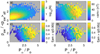 |
Fig. 1 Plots of observed sample numbers, averages and occurrence frequencies, all in bins of normalised solar wind dynamic pressure, p sw/〈p sw〉 that are 0.27 wide and normalised magnetospheric power input (P α /P o) that are 0.135 wide, where 〈p sw〉 and P o are the means of, respectively, p sw and P α for all the data, which are from 1995 to 2019, inclusive. (a) The logarithm to base 10 of the number of 1-minute samples in each bin, log10(N). (b) The mean of the am index, 〈am〉, linearly interpolated to 60 min after the time of the interplanetary observation. (c) The occurrence frequency of interpolated am exceeding the 90th percentile for the distribution for the whole data set of interpolated values for 1995–2019, f[am > q(0.90)]. (d) The occurrence frequency of interpolated am values exceeding the 95th percentile for the whole data set of interpolated values for 1995–2019, f[am > q(0.95)]. |
Paper 2 revealed a second new result about the dynamic pressure. The amplitude of the F-UT equinoctial pattern which, as discussed in Paper 1, is the subject of a great many proposed mechanisms, was shown in Paper 2 to increase linearly with increased p sw. This was arrived at by studying the fit residuals of the best-fit linear regression of P α to am, Δam = am − (sP α + c). The equinoctial pattern seen in am is not present in P α and therefore it is not surprising that it is found in Δam. However, it is a surprise that the amplitude of that pattern increases with p sw. This strongly suggests, but does not prove, that there is a mechanism that generates the equinoctial pattern that is controlled by the dynamic pressure. What is for sure is that the result shown in Paper 2 needs explaining and places a major new constraint on all potential mechanisms. The authors find it very difficult to see how solar wind dynamic pressure could have influenced the conductivity enhancement mechanism that has been proposed as an explanation of the equinoctial variation (Lyatsky et al., 2001; Newell et al., 2002) but we do not rule it out, at least at this stage.
One proposed mechanism which we do rule out is that the equinoctial pattern is caused by variations in the magnetopause reconnection voltage, caused by the sunward tilt of the Earth magnetic axis in the XZ plane, toward or away from the Sun (Crooker & Siscoe, 1986; Russell et al., 2003; Cnossen et al., 2012). We do so because geomagnetic observations show that the equinoctial pattern is not seen in the directly-driven (DP2) currents on the dayside but rather in the nightside DP1 currents and the substorm current wedge. This was first demonstrated by Finch et al. (2008) but the result has since been confirmed by Chambodut et al. (2013) using different data. Chambodut et al. (2013) used the four aσ indices that are compiled from the mid-latitude am stations, but only using stations that are in one of four Magnetic Local Time (MLT) sectors. They showed that the equinoctial pattern (which reveals the effect of the dipole tilt) was strongest for aσ-midnight and weakest for aσ-noon. Finch et al. (2008) used many more magnetometer stations (including polar and auroral stations as well as mid-latitude ones) in order to define the local time and latitude variation more precisely. They found that on the dayside there was no trace of any equinoctial pattern and that it arose most strongly for stations closest to the substorm current wedge. These results have been interpreted as showing that the dipole tilt effect on geomagnetic activity is caused by processes in the tail or by conductivity effects in the nightside auroral ovals and not by changes in the magnetopause reconnection voltage (Lockwood, 2013; Lockwood et al., 2016).
Confirmation of this conclusion is presented in Paper 2, Figure 5 of which shows the F-UT patterns of average transpolar voltage, ΦPC. Because these are average values (covering all phases of the substorm cycle and including northward IMF intervals as well as southward ones) these values must be regarded as long-term averages and so represent steady-state: in which case, these average values of ΦPC equal the averages for the dayside magnetopause reconnection voltage ΦMX and the average reconnection voltage in the cross-tail current sheet ΦTX (Lockwood & Cowley, 1992; Cowley & Lockwood, 1992). Figure 5 of Paper 2 shows that although a semi-annual variation in ΦPC
 (and hence also in ΦMX and
 ΦTX) is clearly present, the UT variation predicted for dipole tilt effects is absent and hence this is not a dipole tilt effect. The third point is that the semi-annual variation in ΦPC
 is actually rather smaller than that in the half-wave rectified dawn-dusk interplanetary electric field E
SW and the estimated power input into the magnetosphere, P
α
. Figure 2 is a summary of data shown in Figure 3 of Paper 2. It shows the normalized variations with fraction of year, F, of E
SW/〈ESW〉, ΦPC/〈ΦPC〉, am/〈am〉 and P
α
/〈P
α
〉 = P
α
/P
o, where the means are taken over all F. Only completely simultaneous data are used which means that the data in all panels are for only the intervals when the DMSP-F13 satellite traversed one or other polar caps. The variations with F in the four panels of Figure 2 are remarkably similar in form and the red and blue lines in the second panel show the same variation is present in ΦPC for both the northern and southern polar caps, as indeed it must always be in steady state and hence long-term averages. Significantly, the relative amplitude of the ΦPC (and hence ΦMX) variation is smaller than that in E
SW and P
α
and so there is no evidence in either the waveform nor the amplitude of the semi-annual variation in ΦMX for a dipole tilt effect on ΦMX. Instead, ΦMX follows that predicted by E
SW and P
α
(which both employ the GSM frame and so contain the Russell-McPherron effect (giving a semi-annual variation) but not the effect of dipole tilt toward and away from the Sun). We conclude that all the evidence is that the Russell-McPherron effect gives the semi-annual variation in ΦMX but there is no evidence for an additional dipole tilt effect on ΦMX. Figure 2 shows that the largest fractional variation is in the am index, implying the am response is amplified. Paper 2 showed that the fit residuals of P
α
to am, Δam, show an almost perfect equinoctial pattern. As mentioned above, at first sight this is not surprising because am shows an equinoctial pattern but P
α
, being computed in the GSM frame, does not. However, P
α
does show a semi-annual variation and that is subtracted in the fit residuals. What is interesting is that when subtracted an equinoctial pattern is revealed (rather than a mixture of an equinoctial and an R-M effect) and this strongly implies that the amplification of the semi-annual variation in am, relative to that in
is actually rather smaller than that in the half-wave rectified dawn-dusk interplanetary electric field E
SW and the estimated power input into the magnetosphere, P
α
. Figure 2 is a summary of data shown in Figure 3 of Paper 2. It shows the normalized variations with fraction of year, F, of E
SW/〈ESW〉, ΦPC/〈ΦPC〉, am/〈am〉 and P
α
/〈P
α
〉 = P
α
/P
o, where the means are taken over all F. Only completely simultaneous data are used which means that the data in all panels are for only the intervals when the DMSP-F13 satellite traversed one or other polar caps. The variations with F in the four panels of Figure 2 are remarkably similar in form and the red and blue lines in the second panel show the same variation is present in ΦPC for both the northern and southern polar caps, as indeed it must always be in steady state and hence long-term averages. Significantly, the relative amplitude of the ΦPC (and hence ΦMX) variation is smaller than that in E
SW and P
α
and so there is no evidence in either the waveform nor the amplitude of the semi-annual variation in ΦMX for a dipole tilt effect on ΦMX. Instead, ΦMX follows that predicted by E
SW and P
α
(which both employ the GSM frame and so contain the Russell-McPherron effect (giving a semi-annual variation) but not the effect of dipole tilt toward and away from the Sun). We conclude that all the evidence is that the Russell-McPherron effect gives the semi-annual variation in ΦMX but there is no evidence for an additional dipole tilt effect on ΦMX. Figure 2 shows that the largest fractional variation is in the am index, implying the am response is amplified. Paper 2 showed that the fit residuals of P
α
to am, Δam, show an almost perfect equinoctial pattern. As mentioned above, at first sight this is not surprising because am shows an equinoctial pattern but P
α
, being computed in the GSM frame, does not. However, P
α
does show a semi-annual variation and that is subtracted in the fit residuals. What is interesting is that when subtracted an equinoctial pattern is revealed (rather than a mixture of an equinoctial and an R-M effect) and this strongly implies that the amplification of the semi-annual variation in am, relative to that in  , does appear to depend on the dipole tilt because the fit residuals do give us the right UT variation for an equinoctial pattern as well as the amplification of the semi-annual variation.
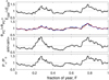 |
Fig. 2 Normalised variations with fraction of a year F for simultaneous data from the years 2001–2003. In each case the data have been averaged into 365 equal-sized bins of time-of year F (one day long for these non-leap years) and then a running mean taken over 27 bins to cover whole solar rotation intervals. The variations are normalised by dividing by the means values for the whole interval. For all parameters, data are only used for the times of the DMSP-F13 polar cap passes giving the transpolar voltage, ΦPC, data. From top to bottom the normalised variations are for: the half-wave rectified dawn-to dusk interplanetary electric field, E SW; the transpolar voltage from F-13; the am geomagnetic index; and the power into the magnetosphere, P α , estimated from near-Earth interplanetary data. The red and blue lines in the panel for ΦPC are for the northern and southern polar caps, respectively. To allow comparison of the amplitudes of these normalise variations, the y scale used in each panel is the same. |
Given there is very strong evidence that the equinoctial variation arises on the nightside and is not found in dayside reconnection voltage nor the associated DP2 currents, we are searching for an alternative explanation for the equinoctial pattern in the am fit residuals. Finch et al. (2008) also showed that these magnetometer deflections in the substorm current wedge that give the equinoctial pattern showed a V SW 2 dependence, which is consistent with the relationship between p sw and the equinoctial Δam patterns revealed in Paper 2. An important clue as to the role of p sw was provided by Caan et al. (1973) who showed that the magnetic energy density in the near-Earth tail lobes was increased by intervals of southward-pointing IMF, as expected for the storage-release system of the magnetosphere, which is the basis of our understanding of the substorm cycle. In the growth phase of substorms, much of the energy that is extracted from the solar wind (P α ) is stored in the near-Earth tail as magnetic flux opened by reconnection in the dayside magnetopause is appended to the tail by the solar wind flow. This energy is subsequently released in substorm expansion phases as that open flux is rapidly re-closed by reconnection in the cross-tail current sheet (see discussion by, e.g., Lockwood, 2019). We know on timescales longer than the substorm cycle (such as the 3-hour time resolution of the am index or greater) that geomagnetic activity is highly correlated with energy input into the magnetosphere, P α averaged over the relevant interval (Lockwood, 2019). In addition, Appendix A of Paper 1 shows that am is highly correlated with both the average and the maximum of the AL and the SML auroral electrojet indices in the 3-hour window it is compiled over and therefore it is dominated by the substorm expansion-phase current wedge and electrojet. Hence the generally-accepted theory of the magnetospheric storage/release system giving substorm cycles predicts that geomagnetic activity, as detected using mid-latitude indices such as am index, will depend on the stored energy in the tail available to drive the substorm expansion phases.
A second finding by Caan et al. (1973) is highly significant – namely that the energy density in the tail is also increased by increased solar wind dynamic pressure. Lockwood (2013) has pointed out that this implies that p SW influences the auroral electrojet and the equinoctial F-UT pattern by constraining the near-Earth tail such that, on appending open flux to the tail lobes of the magnetosphere (during periods of southward IMF), the lobe field (and hence also the stored energy density in the lobes and magnetic shear across the cross-tail current sheet) increases by a greater factor if p SW is large.
To understand the implications of these results, consider a flux F
TL threading a cross section of the tail in one lobe: if, for simplicity, we take the lobe field B
TL to be uniform at the (negative) X coordinate of that cross section, the cross-sectional area of the lobe is A
TL = F
TL/B
TL and the energy stored in the lobe field per unit length is  Hence energy stored in the tail is increased by both increased tail lobe flux, F
TL, and by reduced A
TL. As a point of accuracy, note that F
TL is not quite the same as the total open (polar cap) flux F
pc because there is, in general, open flux F
os that threads the magnetopause sunward of the tail cross-section considered and for a cross-section that is sunward of the tail reconnection X-line there is closed flux F
ca that contributes to F
TL that threads the tail current sheet antisunward of the cross section and sunward of the reconnection X-line. Hence in general F
TL = F
pc + F
ca − F
os. However, in general F
pc ≫ F
ca and F
pc ≫ F
os so F
pc ≈ F
TL. It is known that enhanced dynamic pressure compresses the magnetosphere in a quasi-shape-preserving way (e.g. Roelof & Sibeck, 1993), reducing the near-Earth tail lobe area by a factor f (where f < 1), to
Hence energy stored in the tail is increased by both increased tail lobe flux, F
TL, and by reduced A
TL. As a point of accuracy, note that F
TL is not quite the same as the total open (polar cap) flux F
pc because there is, in general, open flux F
os that threads the magnetopause sunward of the tail cross-section considered and for a cross-section that is sunward of the tail reconnection X-line there is closed flux F
ca that contributes to F
TL that threads the tail current sheet antisunward of the cross section and sunward of the reconnection X-line. Hence in general F
TL = F
pc + F
ca − F
os. However, in general F
pc ≫ F
ca and F
pc ≫ F
os so F
pc ≈ F
TL. It is known that enhanced dynamic pressure compresses the magnetosphere in a quasi-shape-preserving way (e.g. Roelof & Sibeck, 1993), reducing the near-Earth tail lobe area by a factor f (where f < 1), to  . For the same tail lobe flux, the field becomes
  and the energy density stored per unit length of the lobe becomes
  Because f < 1, this means that the energy stored in the tail is increased just by compressing the open flux that is already in the tail which is what Caan et al. (1973) observed. These considerations predict that enhanced dynamic pressure can facilitate the accumulation of magnetic energy in the tail during substorm growth phases and thereby increase geomagnetic activity in the subsequent expansion phases for a given P
α
, which is what Figure 1 shows to occur.
Because f < 1, this means that the energy stored in the tail is increased just by compressing the open flux that is already in the tail which is what Caan et al. (1973) observed. These considerations predict that enhanced dynamic pressure can facilitate the accumulation of magnetic energy in the tail during substorm growth phases and thereby increase geomagnetic activity in the subsequent expansion phases for a given P
α
, which is what Figure 1 shows to occur.
Lastly note that the open flux is controlled by the continuity equation
 (4)where ΦMX is the reconnection voltage across the magnetopause reconnection X line(s) where open flux is generated and ΦTX is the reconnection voltage along the reconnection X-line(s) in the cross tail current sheet where open flux is destroyed (Cowley & Lockwood, 1992). Note that equation (4) is actually Faraday’s law, in integral form, applied to the open-closed field line boundary, OCB. Increasing B
TL near the tail X-line with increased p
SW should increase ΦTX because the magnetic shear across the cross-tail current sheet (≈2 B
TL) is increased. This could reduce the open flux if ΦMX is small but by the continuity equation (4) would just slow the rate of increase if ΦMX is large. In addition, p
SW could increase ΦMX by increasing the reconnection rate or the X-line length in the magnetopause. Hence there is no general relationship between p
SW and the open flux F
pc.
(4)where ΦMX is the reconnection voltage across the magnetopause reconnection X line(s) where open flux is generated and ΦTX is the reconnection voltage along the reconnection X-line(s) in the cross tail current sheet where open flux is destroyed (Cowley & Lockwood, 1992). Note that equation (4) is actually Faraday’s law, in integral form, applied to the open-closed field line boundary, OCB. Increasing B
TL near the tail X-line with increased p
SW should increase ΦTX because the magnetic shear across the cross-tail current sheet (≈2 B
TL) is increased. This could reduce the open flux if ΦMX is small but by the continuity equation (4) would just slow the rate of increase if ΦMX is large. In addition, p
SW could increase ΦMX by increasing the reconnection rate or the X-line length in the magnetopause. Hence there is no general relationship between p
SW and the open flux F
pc.
This series of papers is primarily about annual, semiannual and UT variations in the magnetosphere. Because the solar wind is supersonic and super-Alfvénic, there can be no UT effect generated by the Earth’s rotation on p SW. However, there are semi-annual and annual variations in p SW and these are shown in Figure 3 which gives mean variations as a function of fraction of year F. Figure 3a shows in red the variation of the estimated power input into the magnetosphere, P α , with a weak semi-annual variation and peaks around the equinoxes caused by the R-M effect: this variation has been discussed extensively in Paper 1 and Paper 2. The black line shows the semi-annual variation in the am index which has a considerably enhanced amplitude compared to that in P α , as also discussed in Papers 1 and 2. On the other hand, the blue line shows the dynamic pressure p sw has a predominantly annual variation with peak values in January/December and minimum values June/July. The lack of any equinox peaks in the p sw variation immediately rules out a direct external contribution of p sw to the semi-annual variation in geomagnetic activity. Figure 3b studies the variations of the constituent terms in p sw, given by equation (2). The orange line is m sw which is almost flat (there are extremely weak equinox peaks that may well be a very small axial variation, i.e. associated with Earth’s heliographic latitude, |ΛH|). There are clear near-equinox peaks in the square of the solar wind speed V sw 2, which are consistent with an axial effect and the increased probability of intersecting fast streams when |ΛH| is larger. For the years used to generate Figure 3 (1995–2019) at least, the March peak in V sw 2 is considerably larger than the September one. However, the dominant variation in p sw is set by that in the solar wind number density, N sw, which is caused by the variation over the year of the Sun-Earth distance, r SE. The dashed line shows the normalised variation of 1/r SE 2 which we would expect N sw to follow because there are no sources and sinks of solar wind plasma in interplanetary space.
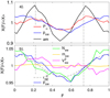 |
Fig. 3 Average variations with fraction of year, F. The data are for 1995–2019, inclusive and are binned into 36 equal width bins of F (each just over 10 days in length) and a 3-point boxcar running mean applied. The data are then normalised by dividing by the mean for all samples. (a) Shows the normalised variation in power input into the magnetosphere, P
α
(red line); the solar wind dynamic pressure, p
sw (blue line) and the am index (black line). (b) The variations of the component terms in p
sw (which is again shown by the blue line): the mean solar wind ion mass, m
sw (orange line); the solar wind number density, N
sw (green line) and the square of the solar wind speed, V
sw
2 (mauve line). The black dashed line is the inverse square of the Sun-Earth distance, |

1.4 UT variations in geomagnetic activity
Paper 1 also showed that there is a persistent UT variation in geomagnetic activity revealed by the am index. This phenomenon has been described many times, with lower activity reported at about 3–9 UT in many papers. In each case, the concern has been the longitudinal evenness of the magnetometer network used, particularly for the Auroral Electrojet indices AE and AL (Davis & Sugiura, 1966; Allen & Kroehl, 1975; Ahn et al., 2000; Ahn & Moon, 2003). However, the results of Lockwood et al. (2019d) show that the am index is by the far the best to employ in this respect and this gives strong support to the reports of the UT variation in am data (Russell, 1989; de La Sayette & Berthelier, 1996; Cliver et al., 2000).
2 Magnetospheric compression by solar wind dynamic pressure
In the present paper, we make use of two models to try to illustrate and elucidate the twin rôles of dynamic pressure p sw and Earth’s dipole tilt ϕ in driving geomagnetic activity: a global magnetohydrodynamic (MHD) numerical model of the magnetosphere and an empirical model of the location of the magnetopause in three dimensions. The latter is used in conjunction with approximations that need to be consistent with each other, but also are consistent with the construction assumptions of the empirical model. Because of these approximations, the results from the empirical model are not as rigorous as those from the MHD model but, nevertheless, allow us to examine some phenomena that are not yet available in the set-up of the MHD model. The approximations used with the empirical model are that the magnetopause is in equilibrium and the so-called “Newtonian approximation,” giving the pressure that the shocked solar wind of the magnetosheath applies to the magnetopause. This approximation is needed to account for the effect that the solar wind is supersonic and super-Alfvénic in the Earth’s frame giving the bow shock upstream of the Earth. The heated, compressed, deflected and slowed solar wind in the magnetosheath, between the bow shock and the magnetopause, can be analytically described by the “gas-dynamic” predictions that assume the magnetic pressure is negligible (Spreiter et al., 1966); however, this assumption is not generally valid (Erkaev et al., 1998).
The Newtonian approximation states that a solar wind velocity of mean ion mass m
sw, number density N
sw and velocity  exerts a pressure p
d on a point on the magnetopause in the direction of the boundary normal at that point,
exerts a pressure p
d on a point on the magnetopause in the direction of the boundary normal at that point,  , of:
, of:
 (5)where the boundary-normal unit vector
  makes an angle ψ with
  and k is the “blunt nose” factor that allows for the loss in pressure as magnetosheath plasma flows around the magnetosphere, and is discussed further below. There are number of different equivalent formulations of this approximation in the literature (Schield, 1969; Sotirelis, 1996; Kartalev et al., 1996; Petrinec & Russell, 1997; Farrugia et al., 1998; Sotirelis & Meng, 1999; Karlsson et al., 2000; Shue & Song, 2002; Merkin et al., 2005; Lu et al., 2015): we here use the formulation in which the total pressure exerted on the magnetopause by the shocked solar wind (including the effect of the static pressure of the undisturbed solar wind in near-Earth interplanetary space outside the bow shock) is given by:
 (6)where p
sw, T
sw, N
sw, and B
sw are the solar wind dynamic pressure, plasma temperature, number density and the interplanetary magnetic field just outside the bow shock in undisturbed interplanetary space; k
B is Boltzmann’s constant and
(6)where p
sw, T
sw, N
sw, and B
sw are the solar wind dynamic pressure, plasma temperature, number density and the interplanetary magnetic field just outside the bow shock in undisturbed interplanetary space; k
B is Boltzmann’s constant and  o the permeability of free space (the magnetic constant). Note that Petrinec & Russell (1997) studied the error in the Newtonian approximation compared to gas-dynamic computations and Lu et al. (2015) have compared it with numerical MHD simulations. Equation (6) is derived by assuming the entire magnetosheath is in equilibrium and by taking the balance of forces on it along the magnetopause boundary-normal direction. Thus the use of the Newtonian approximation expands the requirement that the magnetopause is in equilibrium to the bow shock and the whole magnetosheath also being in equilibrium. This is consistent with the use of the empirical model which is an average location and orientation of the boundary for a given set of prevailing conditions (with no account being taken of the history of those conditions) which is a tacit assumption of equilibrium that would average out transient departures from equilibrium. That having been said, we should note the Cowley & Lockwood (1992) paradigm of flow excitation in the magnetosphere-ionosphere system is that the production of open flux, and its removal from the dayside and appending to the tail lobe, perturbs both the magnetopause and the ionospheric open/closed field line boundary from their equilibrium locations and convection is the motion induced as these boundaries relax back towards their new equilibrium location for given amount of open flux. Hence in this paradigm, the magnetopause is always somewhat perturbed from equilibrium when convection is driven (which is essentially all the time) and adopting equilibrium is almost always a simplifying assumption.
The “blunt nose” k factor is often assumed to be a constant. From gas dynamic calculations around an object of constant shape, Spreiter et al. (1966) computed vales of 0.844 and 0.881 for ratios of the specific heats of 2 and 5/3, respectively. Schield (1969) estimated k to be between 0.7 and 1 and such values have been used in many studies. In general, the erosion of the dayside magnetosphere by magnetic reconnection in the dayside magnetopause when the IMF points southward and consequent appending of open flux to the tail, changes the shape of the magnetosphere and so we should expect the k factor to vary with the magnetopause reconnection voltage and hence the southward component of the IMF in the GSM frame. This has been investigated using a global MHD model of the magnetosphere by Lu et al. (2015) who derived values of 0.8–1.3, depending on [B Z ]GSM and p sw. The values of k > 1 were all for northward IMF and as we are concerned with intervals of enhanced geomagnetic activity such values are not appropriate. Figure 4b of Lu et al. (2015) shows that for p sw = 2 nPa, k varies between about 0.975 for very strongly southward IMF ([B Z ]GSM ≈ −20 nT) and 0.825 for weakly southward IMF ([B Z ]GSM between about −8 nT and zero). We here employ the k = 0.9 but note that the results of Lu et al. (2015) give an uncertainty of order ±0.075 (≈ 8%) due to the effect of IMF [B Z ]GSM. The empirical model of the magnetopause location is valuable because the equilibrium condition means that the pressure exerted by magnetosheath on the magnetopause, p sh, will equal the total pressure inside the boundary (synonymous with energy density) which then can therefore be computed. We use a model of the magnetopause that treats the northern and southern hemispheres separately (Lin et al., 2010) and so is very useful in evaluating the effects of the difference between northern and southern hemispheres of the geomagnetic field. The Lin et al. (2010) model is based on 1226 magnetopause crossings observed between December 1994 and January 2008 by many spacecraft: Cluster, Geotail, GOES, IMP 8, Interball, Los Alamos National Laboratory (LANL), Polar, TC1, Time History of Events and Macroscale Interactions during Substorms (THEMIS), and Wind.
Because of the limitations of the assumption of equilibrium, we here also employ global MHD numerical model simulations of the magnetosphere which also allows us to explore the dynamical processes taking place and how they are influenced by solar wind dynamic pressure and the Earths dipole tilt. We use the Space Weather Modeling Framework (SWMF), developed by the Center for Space Environment Modeling at the University of Michigan to simulate the interaction between solar wind and magnetosphere (described by Tóth et al., 2005, 2012). The SWMF consists of several numerical modules, such as the ideal MHD solver BATSRUS (Block Adaptive Tree Solar-wind Roe-type Upwind Scheme) (Powell et al., 1999; De Zeeuw et al., 2000; Gombosi et al., 2001), an Ionospheric Electrodynamics (IE or RIM) model (Ridley et al., 2002), and the inner magnetosphere Rice Convection Model (RCM; Toffoletto et al., 2003). The SWMF modelling framework has now been tested many times, for example against magnetic field observations from geosynchronous orbit by Rastaetter et al. (2011), using multiple spacecraft covering all areas of the magnetosphere during the 22/23 June 2015 geomagnetic storm by Reiff et al. (2016), by comparison with statistical data ensembles by Ridley et al. (2016) and against empirical field models by Kubyshkina et al. (2019), who also provide a general overview of the development of this modelling capability. The model has been used in a great many studies and in the context of the present paper, we note that Kubyshkina et al. (2015) deployed the model in a study of how dipole tilt influences geomagnetic activity. Specifically, we employ model version SWMF version v20140611. The runs were performed using NASA’s Community Coordinated Modeling Center (CCMC). We study the implications of the empirical model first because many findings are later confirmed using the MHD model. However, the MHD model is set up with a symmetric dipole geomagnetic field and whereas the empirical model treats the two hemispheres separately (Lin et al., 2010) and so can give us information on the effects of the north-south hemispheric asymmetry in the geomagnetic field. This asymmetry is important and growing: the 12th generation of the International Geomagnetic Reference Field (IGFR-12) (Thébault et al., 2015) gives that in 1900 the offset of the geomagnetic dip poles (defined as the points on the Earth’s surface where the magnetic field is vertical) and the geographic (rotational) poles was 19.5° and 18.3° in the north and south hemispheres, respectively, whereas in 2015 these offsets were 3.7° and 25.7°. (Furthermore the northern dip pole has moved through 63.9° of longitude in this interval whereas the southern has moved through 12.6° such that the longitudinal offset between them, which for a geocentric dipole would be 180°, fell from 115.5° to 63.4°). Hence the deviation from a geocentric dipole, and the north-south asymmetry in the field, is significant and has grown.
3 Application of an empirical model of the magnetopause
There are a number of empirical models available that give the location of the magnetopause as a function of the prevailing solar wind conditions (Sibeck et al., 1991; Roelof & Sibeck, 1993; Shue et al., 1997; Kuznetsov & Suvorova, 1998; Shue & Song, 2002; Lin et al., 2010). These models all assume that the magnetopause is in equilibrium by giving a single magnetopause location in any one geocentric direction for a given set of upstream solar wind conditions, with no allowance for time history. We use the model by Lin et al. (2010) because, as discussed above, it treats the two hemispheres separately and that gives us a rare chance to study the effects of north-south asymmetries in the geomagnetic field. The 21 coefficients used by the model are listed in Table 9 of the paper by Lin et al. (2010). The model requires inputs of the IMF B Z component in the GSM frame (we use a range of values but 0 and −6 nT in particular), the solar wind static pressure (we use the mode value of the distribution for 1995–2017 which is 0.015 nPa) and the solar wind dynamic pressure p SW (we use a range of values, and often the mode value for 1995–2017 which is 1.50 nPa) and the dipole tilt angle (we use a range of values, in particular −33, 0 and +33 degrees). In conjunction with these model values we use a blunt-nose k factor of 0.9, as described above.
Figure 4 illustrates the Lin et al. model magnetopause, showing positions for [B Z ]GSM = 0 (in blue) and for southward IMF ([B Z ]GSM = −6 nT, in red), for the mode values of the distributions of observed solar wind static and dynamic pressures over the interval 1995–2017 (respectively, p i = 0.015 nPa and p sw = 1.5 nPa), and for 3 dipole tilt angles, ϕ: close to its smallest value (ϕ = −33°, top panels), close to its largest value ϕ = +33° (bottom panels) and ϕ = 0 (middle panels). The left-hand, middle and right-hand panels are views of Earth (the pale blue dot) in the +Y GSM, −Z GSM and +X GSM directions, respectively, of the GSM frame. (1 R E is a mean Earth radius and equal to 6370 km). The left hand panels are views of the noon-midnight plane (i.e. Y GSM = 0), the middle panels are views of the magnetospheric equatorial plane (i.e. Z GSM = 0) and the right hand panel shows magnetopause locations at X GSM of 5 R E, −10 R E and −25 R E. The left column also shows the tail “hinge point” as a black dot: this is where the tail current sheet (ordered by the solar wind flow) meets the geomagnetic equatorial plane (that orders the near-Earth magnetosphere). For ϕ = ±33° the hinge angle is 147°, for ϕ = 0 it is 180°. The dashed line is the bisector of this hinge angle and we compute the magnetic shear across the tail current sheet at the hinge point from the largest difference in the field perpendicular to this dashed line between two points in opposite lobes along this dashed line. The plots demonstrate the “flaring” of the tail and the earthward erosion of the dayside magnetosphere as the IMF becomes increasingly southward, both caused by the increased voltage with which field lines are opened by magnetic reconnection in the dayside magnetopause (ΦMX) which, in steady state, is the rate at which they are appended to the tail lobe by the magnetic curvature force and then the solar wind flow). Note that Lu et al. (2011) have used global MHD simulations from SWMF and compared to the Lin et al. empirical model and the agreement is generally good but they only used zero dipole tilt and did not consider the effect of hemispheric asymmetry.
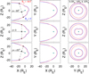 |
Fig. 4 Magnetopause locations in the Geocentric Solar Magnetospheric (GSM) frame of reference from the empirical model by Lin et al. (2010) which treats northern and southern hemispheres separately, so allowing for the hemispheric difference in the offsets of the magnetic poles from the rotation poles. The blue and red lines are for IMF B z (in the GSM frame) of zero and −6 nT, respectively. The plots use the mode values of the distributions of solar wind static pressure p i = N SW k B T SW + B 2/2μ o and dynamic pressures p SW = N SW m SW V SW 2 which are p i = 0.015 nPa and p SW = 1.5 nPa for 1995–2017 (inclusive). The left-hand column gives views of the X GSM Z GSM plane (viewing Earth from the dawn side); the middle column gives views of the X GSM Y GSM plane (viewing Earth from over the north pole) and the right-hand column gives three views in planes parallel to the Z GSM Y GSM plane (viewing Earth from the Sun) at X GSM = 5 R E, −10 R E, and −25 R E. The top row shows results for dipole tilt ϕ = −33°, the middle row for ϕ = 0, and the bottom row for ϕ = +33°. The dashed lines in the left-hand column shows the bisector of the tail “hinge angle”. |
3.1 Tail lobe field intensity and magnetic energy density
The pressure on every point on the magnetopause normal to the boundary is computed using the Newtonian approximation (Eq. (6)). Throughout the analysis in this section, we use the mode values of the distributions of solar wind dynamic and static pressures, as in Figure 4. From assuming pressure balance (equilibrium) throughout the tail, the (anisotropic) pressure (i.e., energy density, ω) can be computed at every point inside the magnetosphere: this is done by assuming that there is pressure balance normal to the magnetopause between the lobe pressure and the pressure on the sheath side of the magnetopause given by the Newtonian approximation. If we assume the dominant pressure is magnetic, which is valid because we consider the tail lobes but exclude the plasma sheet, this energy density is  and hence we can also compute the field in the lobe, B
TL. To simplify the calculations, we consider pressure balance in the YZ plane at a given X, which means we are considering the pressure (energy density) associated with the X-component of the field only. This is a first approximation because total magnetic energy density at any point in the magnetosphere is
and hence we can also compute the field in the lobe, B
TL. To simplify the calculations, we consider pressure balance in the YZ plane at a given X, which means we are considering the pressure (energy density) associated with the X-component of the field only. This is a first approximation because total magnetic energy density at any point in the magnetosphere is
 (7)
(7)
In theory, we could take a tomographic approach and estimate both B X and B YZ at every point in the tail by considering pressure balance along at least two directions at each point. However, this is over-complex for our purposes and not justified when we remember the uncertainties that the assumption of equilibrium will cause. Instead we estimate the first term on the right of equation (7), which is the dominant one in the tail lobe, by evaluating equilibrium pressure balance in YZ plane at each X. We take two approximate approaches to handling the second term. The first is to make only a first order correction for it. At every point inside the magnetosphere the angle that the field makes with the X axis, χ (= arctan (B YZ )/(B X )). When we integrate over a volume τ we get
 (8)
(8)
The first approximation used is that cos2(χ) is unity. By studying the tail at X < −10 R
E the deflections of the field from the ±X direction are generally smaller than about 15° for which  and so using cos2 (χ) = 1 introduces an error in ω
B of less than 7%. However, because cos2 (χ) < 1 this also gives a persistent underestimate which we make a first order correction by multiplying the integral over the volume τ by a constant c
s = 1/(cos2(χ
m
)), where χ
m
is an approximate mean value of |χ|. Using |χ| = 5° gives c
s of 1.08. This method is used only as an order-of-magnitude check on the results of the second method which is to make an estimate of cos2 (χ) at every point. This is done along every diameter of the tail cross section in the YZ plane at a given X. The angle χ at either end of each diameter is given by the magnetopause boundary orientation and we then assume χ varies linearly with distance between these two points. The area-weighted mean of all points in the magnetospheric YZ cross section at each X is than computed. The assumption of a linear variation in χ is a purely pragmatic one, but justified given that χ is small, its effect varies as cos−2(χ) and that in making the correction we are neglecting regions such the plasma sheet where ion and/or electron gas pressure becomes important (so the total energy density ω > ωB).
and so using cos2 (χ) = 1 introduces an error in ω
B of less than 7%. However, because cos2 (χ) < 1 this also gives a persistent underestimate which we make a first order correction by multiplying the integral over the volume τ by a constant c
s = 1/(cos2(χ
m
)), where χ
m
is an approximate mean value of |χ|. Using |χ| = 5° gives c
s of 1.08. This method is used only as an order-of-magnitude check on the results of the second method which is to make an estimate of cos2 (χ) at every point. This is done along every diameter of the tail cross section in the YZ plane at a given X. The angle χ at either end of each diameter is given by the magnetopause boundary orientation and we then assume χ varies linearly with distance between these two points. The area-weighted mean of all points in the magnetospheric YZ cross section at each X is than computed. The assumption of a linear variation in χ is a purely pragmatic one, but justified given that χ is small, its effect varies as cos−2(χ) and that in making the correction we are neglecting regions such the plasma sheet where ion and/or electron gas pressure becomes important (so the total energy density ω > ωB).
We note that the assumption of equilibrium in the tail is a major one, but it matches the same assumption for the magnetosheath (inherent in the Newtonian approximation). Given that the dipole tilt angle will be constantly changing with a cycle period of 24 h it is by no means certain that equilibrium fully applies at any one time and, depending on the timescales to do so, the tail could be in a constant state of evolution. We evaluate the potential effects of this assumption in Section 4 of the present paper using a global numerical MHD model. The top panel of Figure 5 plots the mean energy density 〈ω〉 in the tail as a function of the X coordinate: the average 〈ω〉 is taken over the magnetosphere cross-section in both hemispheres (i.e., all Y GSM and Z GSM inside the magnetopause) or a given X GSM. The different lines are for different combinations of IMF [B Z ]GSM and dipole tilt, ϕ that are input to the magnetopause model. The red, pink, and red dashed lines are for IMF [B Z ]GSM = −6 nT and the blue, cyan and blue dashed lines are for [B Z ]GSM = 0. The red and blue lines are for ϕ = 0 and the effect of appending open flux to the tail during southward IMF can be seen by the raised 〈ω〉 values. The pink and dashed red and cyan and dashed blue are the corresponding variations for ϕ = −33° and ϕ = +33° are very similar but both diverge from the ϕ = 0 case, especially close to Earth.
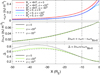 |
Fig. 5 Results of using the Newtonian approximation to obtain the pressure normal to the magnetopause associated with the solar wind static and dynamic pressures (p i and p sw) and assuming the boundary is in pressure equilibrium with the internal pressure we compute the energy density ω at all locations in the magnetospheric tail between X GSE = 0 and X GSE = −50 R E. The top panel shows the average value of ω at a given X GSM for various combinations of the model inputs IMF B z and dipole tilt ϕ. The red and blue lines are for ϕ = 0 and B z = −6 nT and 0, respectively. The pink and dashed red and cyan and dashed blue are the corresponding variations for ϕ = −33° and ϕ = +33°. The middle panel shows the difference in mean energy density for the B z = −6 nT and B z = 0 cases, δ〈ω〉, the black, green and dashed lines being for ϕ = 0, ϕ = +33° and ϕ = −33°, respectively. The bottom panel shows the rise δ〈ω〉 as a ratio of its value for B z = 0, δ〈ω〉/〈ω〉 Bz=0. |
The middle panel of Figure 5 plots the difference δ〈ω〉 between 〈ω〉 for IMF [B Z ]GSM = −6 nT and 〈ω〉 for [B Z ]GSM = 0 (〈ω〉Bz=0). Hence δ〈ω〉 quantifies the additional energy stored in the tail by the enhanced magnetopause reconnection caused by the more southward IMF orientation. The black line is for ϕ = 0. The values of δ〈ω〉 for the near-maximum tilt ϕ (+33°, green line) and the near-minimum ϕ (−33°, black dashed line) are very similar, but not identical and, at all X tailward of −5 R E, δ〈ω〉 is smaller for the large |ϕ| cases than for ϕ = 0. Hence the increased flux in the tail for southward IMF has raised 〈ω〉 by more for ϕ = 0 than for the larger |ϕ| cases. To show the factional increase in stored energy density, the bottom panel of Figure 5 plots δ〈ω〉 as a ratio of the 〈ω〉 value for [B Z ]GSM = 0 (Δ = δ〈ω〉/〈ω〉Bz=0) using the same line colours and types as the middle panel. This reveals that for ϕ = +33° (northern hemisphere summer) the fractional increase in stored energy density is slightly greater than for ϕ = −33° (southern hemisphere summer) at all X < −5 R E. This arises because of the north-south asymmetry in the geomagnetic field that the Lin et al. (2010) model makes allowance for by treating the two hemispheres separately. The fractional rise in stored energy density is greater for ϕ = 0 than for ϕ = −33° or ϕ = +33°. This difference is found at all X below −5 R E and peaks at around −35 R E.
Figure 6 studies the predicted dependencies of the lobe fields on ϕ and IMF [B Z ]GSM in more detail. The top two panels show the maximum magnetic field in the north and south lobes (B N and B S in Figs. 6a and 6b, respectively, where particle pressure is assumed negligible). These values are taken along the bisector of the hinge angle, as shown by the dashed lines in the left-hand plots of Figure 4. They are plotted as a function of ϕ for various values of IMF B z. It can be seen that ϕ has an opposite effect on the maximum field in the two lobes. Figure 6c plots the magnetic shear ΔB (proportional to total current in the current sheet between the lobes): to show the variation with ϕ most clearly, values nave been normalised to the value for ϕ = 0. The magnetic shear is lower for large |ϕ| and the hemispheric asymmetry results in it being lower for ϕ = −33° than for ϕ = +33°. This same behaviour is also seen in the difference in the total energy stored in the tail (between X = −5 R E and X = −50 R E) for IMF [B Z ]GSM = −6 nT and [B Z ]GSM = 0, δW TL (the integral of δ〈ω〉 with X), and its fractional value ΔTL, which are plotted in Figure 6d. The δW TL parameter allows for the change in the volume of the tail V TL which is also given (and does not show as large a variation and asymmetry as the rise in stored energy).
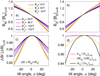 |
Fig. 6 (Top panels) The maximum lobe field along the bisector of the tail hinge angle, evaluated assuming ω = B 2/2μ o and shown as a function of the dipole tilt angle ϕ and for various values of the IMF B z. (a) shows the field in the northern lobe, B N, (b) shows that in the southern lobe, B S, both as a ratio of their values for ϕ = 0. The fall in B N with increasing ϕ is mirrored by a rise in B S, but not quite exactly: this can be seen in part (c) that shows the magnetic shear across the hinge in the current sheet ΔB = |B N| + |B S| which is proportional to the current per unit length in the cross-tail current sheet (again plotted values are normalized to the value for ϕ = 0, [ΔB] ϕ=0. It can be see that ΔB is largest for ϕ = 0 but is also larger for large positive ϕ than large negative ϕ. This is another consequence of the hemispheric asymmetry in the magnetopause model. Part (d) looks at the dependence on ϕ of the difference between the results for IMF B z = −6 nT and B z = 0 of: the total volume of the tail between X GSE = −50 R E and X GSE = 0, V TL; the rise in total stored energy compared to IMF B z = 0 case, δW TL (which is the integral of δω over the volume V TL); and the fractional rise in total energy compared to the B z = 0 case, ΔTL = δW TL/[W TL]Bz=0. Each is again plotted normalized to its value for ϕ = 0 to allow comparisons of the effects of ϕ which in each case shows the same general form as the variation of the magnetic shear, with largest values for ϕ = 0, but slightly larger values for large positive ϕ than for correspondingly large negative ϕ. |
3.2 Equinoctial patterns in tail lobe energy and magnetic shear
The variations with ϕ shown in Figure 6 explain the equinoctial F-UT pattern, as demonstrated by Figure 7. Figure 7a is a reminder of the form of the R-M F-UT pattern, being a plot of sin4(θ/2), where θ is the IMF “clock angle” in the GSM frame θ = arctan(|[B Y ]GSM|/[B Z]GSM), for an IMF in the +Y or –Y direction of the GSEQ frame (B = |[B Y ]GSEQ|) (see Figure 2, Paper 2, Lockwood et al., 2020b). Figure 7b is a F-UT plot of the dipole tilt angle ϕ. Figures 7c and 7d use the F-UT dependence of ϕ shown in Figure 7b with the variations of normalised B N and B S with ϕ for IMF B z = −5 nT that were presented in Figures 6a and 6b, respectively, to plot the F-UT variations of normalised B N and B S (B N/[B N] ϕ=0 and B S/[B S] ϕ=0), predicted by the empirical magnetopause model for equilibrium conditions with IMF B Z = −6 nT and solar wind dynamic pressure, p SW = 1.5 nT.
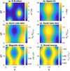 |
Fig. 7 Time-of-year (F) – UT plots based on the dependencies on ϕ shown in Figure 6 for IMF B z = −6 nT and solar wind dynamic pressure, p SW = 1.5 nT. For comparison (a) shows the Russell-McPherron pattern of IMF orientation factor sin4(θ/2) for unit IMF in the +Y or the −Y direction of the GSEQ frame (where θ is the IMF clock angle in the GSM frame). (b) shows the F-UT pattern of the dipole tile angle ϕ. (c) The peak northern hemisphere lobe field along the hinge angle bisector, B N. (d) The peak southern hemisphere lobe field along the hinge angle bisector, B S. (e) The peak magnetic shear across the current sheet at the hinge point, ΔB = B N + B S. (f) The fractional rise ΔTL in total energy stored in the tail (between X GSE = −50 R E and X GSE = −5 R E) compared to for IMF B z = 0. |
Figure 7e shows the maximum magnetic shear across the hinge point between the two lobes ΔB = B N + B S and Figure 7f shows ΔTL, the fractional rise in total stored energy in the tail (between X GSE = −50 R E and X GSE = −5 R E) compared to that for IMF B z = 0. Both these panels show the equinoctial pattern. The study was repeated for a variety of values of the solar wind dynamic pressure p SW between 0.05 nPa and 4 nPa and the pattern of normalised values of ΔB and ΔTL was always as shown in Figure 7, but the absolute values increased linearly, as expected analytically from equation (6) and as shown for observations in Figures 13 and 14 of Paper 2.
Averaging the F-UT patterns in Figures 7b, 7e and 7f over all UT gives the average variations with F shown in Figure 8a and averaging them over all F gives the average UT variations shown in Figure 8b. The blue lines show cos(ϕ), the mauve lines show the maximum magnetic shear ΔB across the hinge point (as a ratio of the value for ϕ = 0, [ΔB] ϕ=0) and the black lines show the fractional increase in total energy stored in the tail (between X GSE = −5 R E and X GSE = −50 R E) for IMF B z = −6 nT compared to B z = 0, ΔTL (as a ratio of [ΔTL] ϕ=0). Both the magnetic shear across the hinge point and the fractional rise in total stored energy show a clear semi-annual variation with clear peaks near to (but not exactly at) the times of minimum |ϕ|. There is also a clear annual variation with larger values predicted around the June solstice than the December one. This is also responsible for moving the peaks in the black and mauve variations towards the summer solstice. This annual variation is discussed further in Section 4. The UT variations for both ΔB/[ΔB] ϕ=0 and ΔTL/[ΔTL] ϕ=0 show a weak minimum at 0-09 UT which is consistent with Figure 13 of Paper 1. The curves for cos(ϕ) show neither of these annual nor UT variations, therefore they are not inherent in the dipole tilt angle. Replacing the magnetopause locations (in both hemispheres) with averages for the two hemispheres at the same X GSM, Y GSM and |Z GSM| causes both the annual and UT variations to disappear and hence both are associated with north-south asymmetry in the magnetopause and hence with north-south asymmetry in the geomagnetic field.
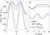 |
Fig. 8 Average variations with (a) time-of-year, F, and (b) Universal Time, UT. The blue lines are for the cosine of the angle tilt angle ϕ, the mauve lines are for the magnetic shear across the hinge point in the tail, ΔB, and the black line is the fractional increase in total energy in the tail (between X GSE = −5 R E and X GSE = −50 R E) for IMF B z of −6 nT compared to zero IMF B z, ΔTL. For ΔB and ΔTL two features are seen that are found in geomagnetic data (see Fig. 15 of Paper 2) but are not present in the cos(ϕ) variation: (1) in the F variation, the December minimum is deeper than the June minimum; (2) the UT variation shows a minimum at 0-8 UT. Both are consequences of the hemispheric asymmetry in the magnetopause model which arises from the hemispheric asymmetry in the geomagnetic field. |
4 Detection of the annual variation in geomagnetic activity
The UT variation predicted above was detected in observations of geomagnetic activity in Paper 1 (Fig. 14). Detecting the annual variation is rather more difficult, but evidence that it is indeed present is given in this section using the am index data and the estimated power input to the magnetosphere P α for 1995–2017, for which the data are quasi-continuous. Data gaps are handled as described in Lockwood et al. (2019a) using their criteria for numbers of samples that restricts errors in P α to 5%. Figures 9b and 9c show the mean values of am/〈am〉1yr and P α /〈P α 〉1yr as a function of fraction of year F and year, using 36 equal-width bins of F and where 〈am〉1yr and 〈P α 〉1yr are the mean values for that year. The top panel shows the daily international sunspot number used to define the solar cycles. As found in Papers 1 and 2, the semi-annual variation is of larger amplitude in am than P α . Also note that there is considerable variability in the separation of the two equinox peaks for am. Figures 9d and 9e study the June-Dec asymmetry by taking mean values in 0.25-year intervals around the June and December solstices: for am these are 〈am〉jun and 〈am〉dec. We then define a solstice asymmetry for am as
 (9)
(9)
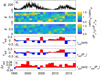 |
Fig. 9 The annual variations of observed am index and inferred power input to the magnetosphere, P α , comparing the solstices in particular. (a) the daily sunspot number, R; (b) the normalised average am index 〈am〉F/〈am〉yr, where 〈am〉F is the average am in 36 equal-bin widths of fraction of year, F, in each year and 〈am〉yr is the average am for that year, color-coded as a function of F and year; (c) the corresponding plot for the power input to the magnetosphere 〈P α 〉F/〈P α 〉yr; (d) a comparison of the means of am in quarter-year intervals around the June and December solstices, 〈am〉jun and 〈am〉dec respectively: the annual value of the ratio r sol(am) is plotted as red/blue bars for years when it was positive/negative, respectively, where r sol(am) = (〈am〉jun − 〈am〉dec)/(〈am〉jun + 〈am〉dec); (e) a comparison of the corresponding ratio for power input to the magnetosphere r sol(P α ) = (〈P α 〉jun − 〈P α 〉dec)/(〈P α 〉jun + 〈P α 〉dec). (f) shows the difference, r sol(am) − r sol(P α ). |
From the model predictions shown in Figure 8a we would expect r sol(am) to be positive. We define r sol(P α ) in the same way, using the corresponding means of P α . The variations in r sol(am) and r sol(P α ) are shown in Figures 9d and 9e, respectively: red histogram bars are for positive values and blue bars are for negative values. It can be seen that there is considerable variability in the polarity of both r sol(am) and r sol(P α ) and that the two vary in a very similar way. Hence the dominant driver of June–Dec asymmetry in am is that in P α , which is largely a matter of chance of when geoeffective solar wind happens to hit Earth. Comparison of (d) and (e) shows that r sol(am) reflects r sol(P α ) very closely we can also see from the previous panels that the equinoctial peaks move toward the summer solstice when r sol(am) is positive, as in Figure 8a. Figure 9f shows r sol(am) − r sol(P α ) which reveals that the asymmetry is consistently a little larger for am than for P α . Thus, although the solstice asymmetry is dominated by the random nature of solar ejecta hitting Earth, there is a persistent bias in that for am that is as predicted in Figure 8a. We attribute this, like the UT variation, to the north-south asymmetry in the geomagnetic field.
5 Global numerical MHD modelling
We employ the BATSRUS global numerical model of the magnetosphere, specifically Space Weather Modeling Framework (SWMF) version v20140611 which deploys the Rice Convection Model. The runs were performed using NASA’s Community Coordinated Modeling Center (CCMC) (Tόth et al., 2005) and the simulation results are available at https://ccmc.gsfc.nasa.gov (runs Henry_Zhou_040616_1, Henry_Zhou_040616_2, Henry_Zhou_040616_2).
At all simulation run times t prior to 100 min, the solar wind conditions were held constant with a 5 nT IMF pointing due southward in GSM coordinates ([B Z ]GSM = B SW = −5 nT), a solar wind number density, N SW of 5 × 10⁶ m−3, a solar wind temperature, T SW of 2 × 10⁵ K and a solar wind speed of V SW = 400 km s−1. The only changes made to these initial conditions were to V SW: starting at t = 100 min, the V SW was ramped up linearly until it reached 800 km s−1 at t = 120 min. It was then held at this value until t = 160 min before again being ramped up linearly to 1200 km s−1 at t = 180 min. and was held at this level until the end of the run at t = 240 min. A summary of model inputs is given in Table 1 which also gives the solar wind dynamic pressure, p sw, the power input to the magnetosphere, P α, and its normalised value P α /P o (where P o = 〈P α 〉1995–2017) for each of the three plateau levels of V SW (400 km s−1, 800 km s−1 and 1200 km s−1).
Model inputs to the CCMC SWMF Magnetosphere model BATSRUS version v20140611 (runs Henry_Zhou_040616_1, _2, and _3) for simulation times t up to 100 min.
Figure 10 places these three plateau levels in context of the observed conditions over the last 22 years. The black line in Figure 10a shows the annual means of P α /P o, where P o is the mean value of P α for all samples in the 22 years. The power input to the magnetosphere, P α , is computed using 1-minute solar wind and IMF data and the theoretical formulation of Vasyliunas et al. (1982) given by equation (1). The coloured pixels give the annual probability density functions (p.d.f.) of P α /P o about these mean values. The horizontal blue, mauve and green lines show P MOD/P o for the three plateau V sw levels, where P MOD is the P α value for the model simulations (given in Table 1): (blue) V sw = 400 km s−1 (for simulation time t < 100 min); (mauve) V sw = 800 km s−1 (for 120 < t < 100 min); and (green) V sw = 1200 km s−1 (for 180 < t < 240 min). Figure 10b shows the distribution of all observed P α /P o for all years (in gray) and again compares it to the three P MOD/P o values. Note that the form and width of the distribution is a strong function of the averaging timescale (Lockwood et al., 2019b) for reasons discussed by Lockwood et al (2019c). Figure 10 shows the variations of the fraction of time that P α exceeds P MOD, f[P α > P MOD]. For V sw = 400 km s−1 (blue line) f[P α > P MOD] varies between 0.033 at sunspot minimum to 0.32 at sunspot maximum; for V sw = 800 km s−1 (mauve line) it varies between 0.001 and 0.051 and for V sw = 1200 km s−1 (green line) it varies between 0 and 0.010. The horizontal coloured dashed lines are the mean values of f[P α > P MOD] over the entire 1995–2017 period.
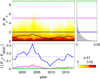 |
Fig. 10 Comparison of the power input to the magnetosphere P MOD for the BATSRUS model run, computed using the model input conditions (listed in Tab. 1) and the theoretical formulation of Vasyliunas et al. (1982), compared to the values from one-minute interplanetary data, P α , computed for 1995–2017. The coloured lines are for the three plateau levels of V sw used in the simulations: (blue) V sw = 400 km s−1 (for simulation time t < 100 min); (mauve) V sw = 800 km s−1 (for 120 < t < 100 min); and (green) V sw = 1200 km s−1 (for 180 < t < 240 min). (a) Annual distributions of P α /P o, where P o is the mean value for all samples in the 22 years. The black line shows the annual means of P α /P o. (b) The distribution of P α /P o for all years (in gray), again compared to the three P MOD/P o values. (c) The variation of the fraction of time that P α exceeds P MOD, f [P α > P MOD]. The horizontal coloured dashed lines are the mean values over the 1995–2017 period. |
5.1 Simulated magnetospheric fields
Figure 11 presents an overview of the BATSRUS predictions for dipole tilts of ϕ = −35° ϕ = 0 and ϕ = +35° in the noon-midnight cross section of the magnetosphere (i.e. the X GSM-Z GSM plane). The colour contours show log10(B) where B is the modelled magnetic field in nT. The open-closed field line boundary at noon and midnight is shown by the black/yellow line in each panel. The mauve lines are open field lines that are mapped from points separated by 7° of latitude along the noon-midnight cross section of the ionospheric polar caps. Each plot in Figure 11 is for simulation run time t = 90 min. The right-hand edge of each plot is at X GSM = +15 R E in the undisturbed solar wind and as X GSM decreases, a steep rise in B is seen at the bow shock. Further decreasing X GSM, we see a fall in B across the magnetosheath and then an even bigger rise in B as we enter the magnetosphere at the magnetopause. We can use this second rise in B to identify the dayside magnetopause. On each plot, the location of the open-closed field line boundary is given and the black dot is the location of the model magnetopause reconnection site, determined as where the boundary normal field, the boundary tangential field and the flow along the boundary all change polarity. For ϕ = 0 the reconnection site in the noon-midnight plane is at a latitude in the GSM frame of [Λ X ]GSM = 0. For ϕ = +34° it is at [Λ X ]GSM = −16° and for ϕ = −34° it is at [Λ X ]GSM = +16°. In all cases the reconnection site sits towards the centre of an extended region of maximum magnetic shear (the maximum difference between any of the three field components) across the magnetopause that is between [Λ X ]GSM of −22° and +22° for ϕ = 0 and between |[Λ X ]GSM| of 0 and 28° in the winter hemisphere for |ϕ| = 34°.
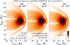 |
Fig. 11 Model simulations of the magnetic field intensity by the BATSRUS global MHD model for dipole tilts ϕ of (a) +35°, (b) 0 and (c) −35°. Each plot is for simulation run time t = 90 min. The open-closed field line boundary is shown in each case and the black dot gives the location of the magnetopause reconnection site. The mauve lines are open magnetospheric field lines separated by 7° along the moon-midnight cross section of the ionospheric polar caps. A summary of model inputs is given in Table 1. |
The open field lines in Figure 11 illustrate a key point concerning the fraction of the open flux that is appended to the tail lobe and the fraction that threads the dayside magnetopause (referred to as flux F os in Sect. 1.3). In the symmetric case in the X GSM-Z GSM plane (ϕ = 0, Fig. 11b), 5 of the 7 illustrative open field lines in each hemisphere thread the lobe at the left-hand edge of the plot at X GSM = −30 R E, and two thread the magnetopause sunward of X GSM = −30 R E. For the asymmetric cases the situation is different. In the summer hemisphere (the northern in Fig. 11a and the southern in Fig. 11c) a smaller fraction is appended to the lobe because a larger fraction threads the dayside magnetopause (3 of the illustrative field lines thread the lobe at X GSM = −30 R E and 4 thread the magnetopause sunward of X GSM = −30 R E). Conversely, in the winter hemisphere (the southern in Fig. 11a and the northern in Fig. 11c) a larger fraction is appended to the lobe and a smaller fraction threads the dayside magnetopause (5 of the illustrative field lines thread the lobe at X GSM = −30 R E and 2 thread the magnetopause sunward of X GSM = −30 R E). Thus total flux in the near-Earth lobes is lower for ϕ = −35° and ϕ = +35° (8 illustrative field lines) than for ϕ = 0 (10 illustrative field lines).
This effect is quantified more accurately in the following section and in three dimensions (i.e., considering the open flux at |Y GSM| > 0, away from the noon-midnight plane). The cause is readily inferred from animations of Figure 11 for different simulation times, t: in the large |ϕ| cases the reconnection site is shifted from the subsolar point into the winter hemisphere. This shift of the reconnection site (and of the location of maximum magnetic shear across the dayside magnetopause) into the winter hemisphere was found in MHD simulations by Park et al. (2006) and Hoilijoki et al. (2014) and in observations by Trattner et al. (2012), Zhu et al. (2015) and Kitamura et al. (2017). In the winter hemisphere, the curvature force acting to straighten newly-opened field lines acts in the same direction as the near-magnetopause magnetosheath flow and the field lines evolve rapidly into the tail lobe. In addition, the distance around the magnetopause from the reconnection site to a point on the tail magnetopause at a given X GSM is smaller. On the other hand, for open field lines evolving into the summer hemisphere, the sheath flow and magnetic curvature forces are acting in opposite directions close to the X-line and the initial motion towards the tail lobe is slow. In addition, the distance around the magnetopause from the reconnection site to a point on the tail magnetopause at a given X GSM is larger. The effect is that more open field lines at any one instant have evolved into the tail lobe in the winter hemisphere than in the summer hemisphere. For the ϕ = 0 case, the reconnection site is at the subsolar point and the situation in both hemispheres is similar to the winter hemisphere case for larger |ϕ| and field lines evolve more rapidly into the tail lobe.
5.2 Magnetic fluxes and total energy in the tail lobes
Figure 12 shows the field magnitude B in cross sections of the geomagnetic tail at the same simulation time as Figure 11 (t = 90 min). The rows are for X
GSM of (from top to bottom) −10 R
E, −15 R
E, −20 R
E, and −25 R
E. The columns are for dipole tilts of (left) ϕ = +35°, (middle) ϕ = 0 and (right) ϕ = −35°. In each plot, the outer edge of the outer ring is the bow shock and the inner high- region is the magnetosphere and the two tail lobes, separated by the low-field plasma sheet, can be clearly seen. At all X
GSM the field in the “winter” lobe (south for ϕ = +35°, north for ϕ = −35°) is similar to that for the ϕ = 0 case whereas for the “summer” lobe (north for ϕ = +35°, south for ϕ = −35°) it is always considerably lower. These variations of the field strength with ϕ are qualitatively consistent with the deduction in Figures 6a and 6b from the magnetopause model. The area of the summer lobe is always larger and the well-known curvature of the cross-tail current sheet at large ϕ can be seen clearly. Note that the colour scale is reduced for increasingly negative X
GSM and so the change in colours does not fully describe the decrease in field strength with distance down the tail.
region is the magnetosphere and the two tail lobes, separated by the low-field plasma sheet, can be clearly seen. At all X
GSM the field in the “winter” lobe (south for ϕ = +35°, north for ϕ = −35°) is similar to that for the ϕ = 0 case whereas for the “summer” lobe (north for ϕ = +35°, south for ϕ = −35°) it is always considerably lower. These variations of the field strength with ϕ are qualitatively consistent with the deduction in Figures 6a and 6b from the magnetopause model. The area of the summer lobe is always larger and the well-known curvature of the cross-tail current sheet at large ϕ can be seen clearly. Note that the colour scale is reduced for increasingly negative X
GSM and so the change in colours does not fully describe the decrease in field strength with distance down the tail.
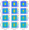 |
Fig. 12 Cross sections of the tail from the BATSRUS model runs showing the magnetic field intensity, B. The rows are for X GSM (=X GSE) of (from top to bottom) −10 R E, −15 R E, −20 R E, and −25 R E. The columns are for dipole tilts ϕ of (left) +35°, (middle) 0 and (right) −35 °. The outer ring is the bow shock and the two tail lobes, separated by the low-field plasma sheet can be clearly seen. At all X GSM, the field in the “winter” lobe (south for ϕ = +35°, north for ϕ = −35°) is similar to that for the ϕ = 0 case (and sometimes very slightly enhanced), whereas for the “summer” lobe (north for ϕ = +35°, south for ϕ = −35°) it is always considerably lower. |
It is important to stress that BATSRUS includes no north-south asymmetry in the geomagnetic field and so the results for ϕ = −35° in the north/south hemisphere are the same as for ϕ = +35° in the south/north hemisphere (i.e., in the winter/summer hemisphere, respectively). Henceforth we only present results for ϕ = +35° and then study the two hemispheres.
Figure 13 plots the magnetic flux threading the tail lobes as a function of X (the lobes being identified by the polarity of the B
X
component). The flux was then estimated by integrating  over the cross-sectional area of the lobe. Taking cross sections at a given X, the elements of area are in the ZY plane, da
YZ
and the normal field to those elements is B
x
, hence
over the cross-sectional area of the lobe. Taking cross sections at a given X, the elements of area are in the ZY plane, da
YZ
and the normal field to those elements is B
x
, hence  . One polarity of B
X
is considered at a time to separate out the northern and southern lobes. We found the most useful way to distinguish the lobes from the central plasma sheet, the magnetosheath and the solar wind was to require the total particle energy density, ω
P (for this simulation and for the X values that we are interested in) to be below 2 × 10⁻¹⁰ J m−3. Sampled comparisons with a magnetopause locator provided by CMCC were extremely close. To integrate, we first applied a 2-D interpolation linear scheme to
. One polarity of B
X
is considered at a time to separate out the northern and southern lobes. We found the most useful way to distinguish the lobes from the central plasma sheet, the magnetosheath and the solar wind was to require the total particle energy density, ω
P (for this simulation and for the X values that we are interested in) to be below 2 × 10⁻¹⁰ J m−3. Sampled comparisons with a magnetopause locator provided by CMCC were extremely close. To integrate, we first applied a 2-D interpolation linear scheme to  and to
  to give a higher spatial resolution grid with separations of 1% of the MHD model grid-point separations.
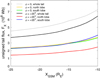 |
Fig. 13 The variation of the total magnetic flux in the tail lobes and in the whole tail as a function of X GSM for ϕ = +35° and ϕ = 0 from the BATSRUS model runs at simulation time t = 90 min. (Because the model uses a symmetric intrinsic geomagnetic field the ϕ = −35° case gives the same information as the ϕ = +35° case with the hemispheres flipped). For ϕ = 0 the variation for the two lobes is the same (the orange line has been offset from the green by a linewidth so it can be seen). For ϕ = +35° the flux is lower in the northern (“summer”) lobe than the southern (“winter”) and the sum of the two (the black line) is lower than the sum for ϕ = 0 (the black line). |
The orange and green lines are for the north and south lobes and ϕ = 0 and the black line is the sum of the two. All fluxes fall with increasingly negative X because of flux crossing the cross tail current sheet (from south to north sunward of the tail reconnection X-line and north to south tailward of the X-line: the former flux was referred to as F
ca in Sect. 1.3). The red, blue and grey lines are the same for ϕ = +35°, being for the north, south and both lobes, respectively. (The symmetry of the model means that for ϕ = −35° the plots are the same but the north and south hemisphere variations are swapped.) The flux variation for ϕ = +35° in the southern (winter hemisphere) is roughly the same as for both hemispheres for ϕ = 0, but the lobe flux in the north (summer hemisphere) is considerably smaller and so, therefore, is the total. Table 2 quantifies the effect noted here and in Figure 11 by computing the fraction of the open magnetospheric flux (which by Maxwell’s law  must be the same in the two hemispheres) that threads each tail lobe at X
GSM = 10 R
E at simulation time t = 90 min. For ϕ = 0, the percentage is 62.33% for both the northern and southern lobe, whereas for ϕ = +35° it is 48.30% for the northern (summer) lobe and 77.95% for the southern (winter) lobe. For the two hemispheres combined, the percentages are 62.33% for ϕ = 0 and 63.13% for ϕ = +35°. Figure 13 shows that for |ϕ| = 35°, the difference between the flux threading the summer and winter tail lobes at X
GSM < −15 R
E is roughly constant at about 0.9 × 10⁸ Wb. The newly-opened flux on the summer side of the magnetopause reconnection site (that is shifted into the winter hemisphere, as shown in Fig. 11) increases in velocity from zero at the reconnection site to approximately V = 80 km s−1 at the magnetic equator, a distance of 2 × 10⁷ m. Thus field lines evolving into the summer lobe take of order 500 s for evolve from the reconnection site to the magnetic equator in the |ϕ| = 35° cases, a motion aided by the field curvature force but opposed by the magnetosheath flow. At the estimated reconnection voltage of 95 kV, this means that there is a flux of 500 × 95 × 103 = 0.475 × 10⁸ Wb that is destined for the summer lobe but is still threading the dayside magnetopause in the winter hemisphere between the reconnection X-line and the geomagnetic equator. This alone accounts for over half of the difference in fluxes threading the two lobes.
must be the same in the two hemispheres) that threads each tail lobe at X
GSM = 10 R
E at simulation time t = 90 min. For ϕ = 0, the percentage is 62.33% for both the northern and southern lobe, whereas for ϕ = +35° it is 48.30% for the northern (summer) lobe and 77.95% for the southern (winter) lobe. For the two hemispheres combined, the percentages are 62.33% for ϕ = 0 and 63.13% for ϕ = +35°. Figure 13 shows that for |ϕ| = 35°, the difference between the flux threading the summer and winter tail lobes at X
GSM < −15 R
E is roughly constant at about 0.9 × 10⁸ Wb. The newly-opened flux on the summer side of the magnetopause reconnection site (that is shifted into the winter hemisphere, as shown in Fig. 11) increases in velocity from zero at the reconnection site to approximately V = 80 km s−1 at the magnetic equator, a distance of 2 × 10⁷ m. Thus field lines evolving into the summer lobe take of order 500 s for evolve from the reconnection site to the magnetic equator in the |ϕ| = 35° cases, a motion aided by the field curvature force but opposed by the magnetosheath flow. At the estimated reconnection voltage of 95 kV, this means that there is a flux of 500 × 95 × 103 = 0.475 × 10⁸ Wb that is destined for the summer lobe but is still threading the dayside magnetopause in the winter hemisphere between the reconnection X-line and the geomagnetic equator. This alone accounts for over half of the difference in fluxes threading the two lobes.
The percentages of open magnetospheric flux threading the magnetopause (MP) in the north and south hemispheres at X GSE > −10 R E and run time t = 90 min.
Figure 14 uses the same colour scheme as Figure 13, but shows the corresponding variations for the total magnetic energy density per unit X, (dW B)⁄dX (in terms of the energy density ω, dW B/dX = ωA TL, where A TL is the cross-sectional area of the lobe). Note that Figure 12 shows there are variations with X GSM in both B (and so B 2/2μ o) and in cross-sectional area and both contribute to dW B/dX. Integrating over the 15 R E length of the tail shown reveals that total magnetic energy W B is 20% larger for the ϕ = 0 case than for the |ϕ| = 35° cases which is a larger effect than the 5% effect found using the empirical magnetopause model in Section 2.
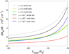 |
Fig. 14 The same as Figure 13 for the total magnetic energy stored in unit length of the tail, dW B/dX from the BATSRUS model runs at simulation time t = 90 min. As for the magnetic flux in the tail, the sum of the two is lower for the ϕ = +35° case than the ϕ = 0 case. The total energy W B over the 15 R E length shown is 20% larger for the ϕ = 0 case which is a larger effect than the 5% effect found using the empirical magnetopause model (see Fig.5). |
Figure 15 studies the maximum magnetic shear across the tail current sheet as a function of X GSM and Y GSM. The left panel is for ϕ = 0, the middle panel for ϕ = +35° and the right panel shows the difference between the two. The right panel therefore shows where and by how much the cross tail current is decreased when ϕ = ±35° compared to when ϕ = 0: it is mainly reduced down the centre of the tail which is likely to be where and why the tail reconnection voltage is reduced.
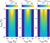 |
Fig. 15 The magnetic shear ΔB across the cross-tail current sheet as a function of X GSM and Y GSM from the BATSRUS model runs at simulation time t = 90 min. The left panel is for ϕ = 0, the middle panel for ϕ = +35° and the right panel shows the difference between the two. |
5.3 Reconnection voltage and tail energy density changes caused by solar wind velocity increases
In this section we study how the reconnection and transpolar voltages behave for ϕ = ±35° and ϕ = 0 with simulation time. In the model simulation runs, the input solar wind velocity V SW was ramped up linearly from 400 km/s to 800 km/s between simulation times t of 100 min and 120 min and then from 800 to 1200 km/s at t between 160 and 180 min. All these timings are for interplanetary space at X GSM = 30 R E. Figure 16a shows the consequent variation in solar wind dynamic pressure p sw, the vertical pink lines bounding the increases in V SW. The increases in V SW also increase the dawn-to-dusk electric field [E Y ]GSM = V SW [B Z ]GSM. Figure 16b shows the variation of the voltage placed across the magnetopause ΦM = [E Y ]GSM[ΔY]GSM = V SW [B Z ]GSM[ΔY]GSM, where [ΔY]GSM is the modelled width of the magnetopause in the Y GSM direction, taken here at the average X GSM of the tail reconnection site, X R. The tail reconnection line is identified as where [B X ]GSM, [B Z ]GSM, and [V X ]GSM all change polarity. Note that the width of the tail [ΔY]GSM is slightly greater for ϕ = 0 than for ϕ = ±35° and this is reflected in the ΦM values shown by the green and black lines, respectively, in Figure 16b.
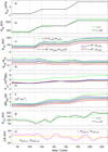 |
Fig. 16 Modelled effect of solar wind speed changes. Between simulation times t of 100 min and 120 min and between 160 min and 180 min the solar wind velocity V SW was ramped up linearly. These times are marked by vertical pink lines. (a) The resulting variation in solar wind dynamic pressure, p sw. (b) The voltage placed across the magnetosphere by the solar wind flow, ΦM = V SW[B Z ]GSMΔY M, where ΔY M is the width of the magnetosphere in the Y direction of the GSM frame (here taken to be at the average X GSM of the tail reconnection X- line, X R). The green line is for ϕ = 0 and the black line for ϕ = 35°. (c) The transpolar voltages across the ionospheric polar caps. The green line is for ϕ = 0 for which the voltages across the northern and southern polar caps, [ΦPC]N and [ΦPC]S, are essentially identical. The blue and red and lines are [ΦPC]N and [ΦPC]S for ϕ = +35° (i.e., for the summer and winter hemispheres). The area between the two is shaded grey and the black line is the average of [ΦPC]N and [ΦPC]S. This colour scheme is used in all panels (d)-(f) showing equivalent parameters. (d) The reconnection efficiencies, [ΦPC]N/ΦM and [ΦPC]S/ΦM. (e) The total open magnetic fluxes in the northern and southern hemispheres [F PC]N and [F PC]S. (f) The magnetic energy stored per unit length of the tail at X GSM ≈ X R, the average X GSM of the tail reconnection X-line, [dW BX /dX]N and [dW BX /dX]S. (g). The tail current sheet reconnection voltages, ΦTX. (h) The difference in reconnection voltages for the ϕ = 0 and ϕ = 35° simulations, ΔΦ: the orange line is for the inferred reconnection voltages in the dayside magnetopause, ΔΦ = [ΦMX] ϕ=0 − [ΦMX] ϕ=35, the mauve line is for the inferred reconnection voltages in the nightside cross-tail current sheet, ΔΦ = [ΦTX] ϕ=0 − [ΦTX] ϕ=35. The vertical pink lines in panels (c)–(h) bound the solar wind velocity increases lagged by the inferred average propagation delay of 8 min. The average tail reconnection site varied between X GSM = −21 R E and X GSM = −24 R E for ϕ = 0 and at X GSM between −17 R E and −20 R E for ϕ = 35°. |
Figure 16c shows the voltages across the two ionospheric polar caps, [ΦPC]N and [ΦPC]S that are generated by the Ridley Ionosphere Model (RIM) at simulation times dt = 1 min apart as a standard product of the model. For the case of zero dipole tilt, ϕ = 0, [ΦPC]N and [ΦPC]S are essentially identical and are given by the green line. However, for the case of ϕ = +35°, [ΦPC]N (the transpolar voltage in the summer hemisphere, red line) is consistently smaller than [ΦPC]S (the transpolar voltage in winter hemisphere, blue line) which is very similar to that for ϕ = 0. (Note that for the case of ϕ = −35°, identical plots were obtained with [ΦPC]N and [ΦPC]S swapped.) The effects of the two ramps of increasing V SW can be seen as upward ramps in [ΦPC]N and [ΦPC]S after a mean lag dt of 8 min. which accounts for propagation from X GSM = 30 R E to the nose of the magnetopause and across the magnetosheath and the subsequent rise time of the transpolar voltages, showing the derived transpolar voltages are dominated by the magnetopause reconnection. Note that the vertical pink lines have been shifted by this lag in parts (c)–(h) of Figure 16. Figure 16c plots the reconnection efficiencies, estimated as ΦPC(t)/ΦM(t − dt). These reconnection efficiency estimates are almost constant showing that the transpolar voltages ΦPC are largely set by the voltage across the magnetosphere ΦM. However, this is not quite true, as each upward ramp in V SW causes a slight ramped decrease in the reconnection efficiency.
The tendency for the simulated transpolar voltage (often called the cross-cap potential, although it is in reality a potential difference, i.e. a voltage) to be greater in the winter hemisphere, seen in Figure 16d, was also noted in BATSRUS model by Zhang et al. (2007) and attributed to the lower conductivity in the winter ionosphere. These authors also noted the same effect was seen, albeit to a lesser extent in the statistical DMSP-based Ionospheric Convection Model (DICM) (Papitashvili & Rich, 2002) but only when [B Y ]GSM is large (which does not apply in this case) and the results from the Assimilative Mapping of Ionospheric Electrodynamics (AMIE) technique (Richmond & Kamide, 1988) for the storm that they numerically simulated tended to lie close to the average of [ΦPC]N and [ΦPC]S.
The difference between [ΦPC]N (summer hemisphere transpolar voltage) and [ΦPC]S (winter hemisphere transpolar voltage) shown by the red and blue lines in Figure 16d for ϕ = 35°, raises an important point. By Faradays law, “voltage” is synonymous with “flux transfer rate”. (Incidentally, that is why it is important to stress that the name cross-cap potential is physically misleading.) In steady state, the flux transfer rate into the tail must be the same in the two hemispheres: this means that a difference between the two transpolar voltages is an inherently non-steady state situation and so we should not expect to see a hemispheric difference in transpolar voltages in statistical models that average in such a way as to tend to a steady state description (an assumption often made tacitly by assuming that there is a single transpolar voltage for a given set of interplanetary conditions). An additional factor is Maxwell’s equation  (the non-existence of magnetic monopoles) which means that the total open flux in the two hemispheres must always be identical ([F
PC]N = [F
PC]S). This is shown to be true to for the global MHD simulations in Figure 16e (any slight differences in the ϕ = +35° case are associated with numerical errors in field line mapping) but note that the total open flux for ϕ = +35° (red black and blue lines) is consistently smaller than for ϕ = 0 (green line) by a factor of about a quarter.
(the non-existence of magnetic monopoles) which means that the total open flux in the two hemispheres must always be identical ([F
PC]N = [F
PC]S). This is shown to be true to for the global MHD simulations in Figure 16e (any slight differences in the ϕ = +35° case are associated with numerical errors in field line mapping) but note that the total open flux for ϕ = +35° (red black and blue lines) is consistently smaller than for ϕ = 0 (green line) by a factor of about a quarter.
At the magnetopause, the transfer of open field lines into the tail is controlled by the unwinding of the curvature force on newly-opened field lines and then the magnetosheath flow. Tangential stress balance tests at the magnetopause (Paschmann et al., 1986; Lockwood & Hapgood, 1998; Blagau et al., 2015; Sonnerup et al., 2016) demonstrate that the ionospheric conductivity can has no influence on the balance of forces on field lines at the magnetopause and differences in transfer rates at the magnetopause and in the ionosphere caused by ionospheric conductance demonstrate their decoupling by induction effects (i.e., changes in the magnetic field between the magnetopause and the ionosphere) (Lockwood & Cowley, 1992). Any reduced flux transfer rate along the magnetopause in the summer hemisphere must lead to a faster accumulation of flux in the winter lobe, F N, compared to that in the summer lobe, F S. This can be seen to be occurring in Figure 16f which plots the magnetic energy stored in unit length [dW BX /dX]N and [dW BX /dX] of the two lobes at X GSM ≈ X R, the X GSM of the tail reconnection X-line: the energy stored in the winter hemisphere lobe field near the X-line for ϕ = +35° (the blue line) is slightly lower than that stored in either lobe for ϕ = 0 (the green line), but the energy stored in the summer lobe (the red line) is considerable lower. All these energies ramp up following the solar wind increases, but the average for ϕ = 0 is always greater than, and increases with increased p SW by a larger factor, than for ϕ = +35°. Hence the effect of tilt is consistent with that deduced from the magnetopause model (see Fig. 6). Given the pressure on the tail magnetopause exerted by the magnetosheath, this means that the current sheet between the two lobes will migrate towards the summer hemisphere, as noted in simulations using the same MHD model by Ridley et al. (2004). This motion is also found in the simulations presented here for ϕ = ±35°. Note however, that it is the rate of transfer of field lines along the magnetopause, not that in the ionosphere, that is causing this – and hence any hemispheric difference in ionospheric transpolar voltage caused by ionospheric conductivity is not a factor in these changes in the tail, as described by Lockwood & Cowley (1992), that difference is accounted for by the inductive decoupling caused by changes to open field lines between the tail lobe and the ionosphere (see also Lockwood & Morley, 2004).
Because of Maxwell’s equation  the rate at which open field lines are generated in the two hemispheres must always be identical, being equal to the voltage across the magnetopause reconnection line (or potentially several spatially separated lines), ΦMX
, in both hemispheres. The modelled accelerated flows along the dayside magnetopause show that the dipole tilt shifts the magnetopause reconnection site into the winter hemisphere in the simulations. As a result, for the newly-opened field lines evolving towards the winter hemisphere, the magnetosheath flow and the magnetic curvature force act in the same direction and the field lines evolve rapidly toward the winter tail lobe. On the other hand, for open field lines on the other side of the magnetopause X-line, the curvature force initially has to act against the magnetosheath flow (which has a component directed away from the subsolar point and back towards the X-line) and open field lines evolve more slowly towards the summer lobe. As a result, as indicated by Figure 11, more of the open flux threads the dayside magnetopause in the summer hemisphere than in the winter hemisphere and, consequently, less flux threads the summer lobe than the winter lobe. This is quantified in Table 2 for the simulation time t = 90 min: for ϕ = ±35°, 52% of the open flux threads the dayside magnetopause sunward of X
GSM = −10 R
E in the summer hemisphere whereas this figure is only 22% for the winter hemisphere. By comparison, for ϕ = 0 this percentage is 38% in both hemispheres. Hence the winter tail lobe anti-sunward of X
GSM = −10 R
E contains more flux for ϕ = ±35° (100–22 = 78%) than that in the summer tail lobe (100–52 = 48%), a ratio of (78/48) ≈ 1.6.
the rate at which open field lines are generated in the two hemispheres must always be identical, being equal to the voltage across the magnetopause reconnection line (or potentially several spatially separated lines), ΦMX
, in both hemispheres. The modelled accelerated flows along the dayside magnetopause show that the dipole tilt shifts the magnetopause reconnection site into the winter hemisphere in the simulations. As a result, for the newly-opened field lines evolving towards the winter hemisphere, the magnetosheath flow and the magnetic curvature force act in the same direction and the field lines evolve rapidly toward the winter tail lobe. On the other hand, for open field lines on the other side of the magnetopause X-line, the curvature force initially has to act against the magnetosheath flow (which has a component directed away from the subsolar point and back towards the X-line) and open field lines evolve more slowly towards the summer lobe. As a result, as indicated by Figure 11, more of the open flux threads the dayside magnetopause in the summer hemisphere than in the winter hemisphere and, consequently, less flux threads the summer lobe than the winter lobe. This is quantified in Table 2 for the simulation time t = 90 min: for ϕ = ±35°, 52% of the open flux threads the dayside magnetopause sunward of X
GSM = −10 R
E in the summer hemisphere whereas this figure is only 22% for the winter hemisphere. By comparison, for ϕ = 0 this percentage is 38% in both hemispheres. Hence the winter tail lobe anti-sunward of X
GSM = −10 R
E contains more flux for ϕ = ±35° (100–22 = 78%) than that in the summer tail lobe (100–52 = 48%), a ratio of (78/48) ≈ 1.6.
In steady state, the transpolar voltages would have to be the same in the two hemispheres and both would equal the reconnection voltage in the dayside magnetopause and in the cross-tail current sheet ([ΦPC]N = [ΦPC]S = ΦMX
= ΦTX). For non-steady conditions, Faraday’s law, applied to the boundary of the open field line region (the polar cap) becomes a continuity equation for the open flux, F
PC, given by equation (4). We computed the tail reconnection voltage ΦTX in three separate ways. Firstly, for simulation times dt = 1 min apart, we identified the tail X-line in the model simulations, defined by where [B
X
]GSM, [B
Z
]GSM and [V
X
]GSM all swapped polarity. The average X
GSM of the tail reconnection site, X
R, varied between −21 R
E and −24 R
E in the ϕ = 0 simulations and between −17 R
E and −19 R
E for ϕ = 35°. Note that this reconnection in the model is associated with numerical diffusion in the MHD code and so we do not place great significance on these X-line positions in terms of the real magnetosphere, only in the simulations. We then computed integrated  along the length of the model X-line where
  is the electric field along the X-line (the reconnection rate) in its own rest frame. There are always numerical errors associated with this kind of calculation (Ridley et al., 2010) because it relies on correct identification of the X-line and its motion (which is often slow, meaning its motion is quantised by the 0.4 R
E spatial grid resolution of the model and linear interpolation was required). We also computed ΦTX using Faraday’s induction law applied to the two tail lobes separately
is the electric field along the X-line (the reconnection rate) in its own rest frame. There are always numerical errors associated with this kind of calculation (Ridley et al., 2010) because it relies on correct identification of the X-line and its motion (which is often slow, meaning its motion is quantised by the 0.4 R
E spatial grid resolution of the model and linear interpolation was required). We also computed ΦTX using Faraday’s induction law applied to the two tail lobes separately
 (10)where F
L is the magnetic flux threading the lobe at X
GSM = X
R,
(10)where F
L is the magnetic flux threading the lobe at X
GSM = X
R,  is the electric field in the magnetopause at X
GSM = X
R (in its rest frame) surrounding that lobe and
is the electric field in the magnetopause at X
GSM = X
R (in its rest frame) surrounding that lobe and is an element of length in that magnetopause boundary and the integration is carried out along the magnetopause segment MP at X
GSM = X
R from the point where it meets the cross-tail current sheet on the dawnside to where it meets it on the dusk side. The calculation was carried out for the northern and southern lobes separately, and depends on correctly identifying the magnetopause and its motion, which causes similar problems to the previous X-line calculation. Lastly, we used equation (5) with the assumption that ΦMX was equal to ΦPC in the winter hemisphere, [ΦPC]S (shown in Fig. 16c). By Faradays law, ΦMX = [ΦPC]S means that there is no build up nor decay of magnetic flux in the winter (southern) hemisphere between the magnetopause reconnection site and the points that map to the dawn-dusk cross-section of the winter ionospheric polar cap across which [ΦPC]S is measured, in other words the winter dayside open flux is in steady state. This assumption was tested by computing the rate of change of magnetic flux threading the dayside magnetopause sunward of X
GSM = 0: it was found for the winter hemisphere this varied between 4 kV and −4 kV with an average value of 0.4 kV. Hence assuming ΦMX = [ΦPC]S (in this case where the southern polar cap is in winter) is accurate to within 5% at any one t and to within 0.5% on average.
is an element of length in that magnetopause boundary and the integration is carried out along the magnetopause segment MP at X
GSM = X
R from the point where it meets the cross-tail current sheet on the dawnside to where it meets it on the dusk side. The calculation was carried out for the northern and southern lobes separately, and depends on correctly identifying the magnetopause and its motion, which causes similar problems to the previous X-line calculation. Lastly, we used equation (5) with the assumption that ΦMX was equal to ΦPC in the winter hemisphere, [ΦPC]S (shown in Fig. 16c). By Faradays law, ΦMX = [ΦPC]S means that there is no build up nor decay of magnetic flux in the winter (southern) hemisphere between the magnetopause reconnection site and the points that map to the dawn-dusk cross-section of the winter ionospheric polar cap across which [ΦPC]S is measured, in other words the winter dayside open flux is in steady state. This assumption was tested by computing the rate of change of magnetic flux threading the dayside magnetopause sunward of X
GSM = 0: it was found for the winter hemisphere this varied between 4 kV and −4 kV with an average value of 0.4 kV. Hence assuming ΦMX = [ΦPC]S (in this case where the southern polar cap is in winter) is accurate to within 5% at any one t and to within 0.5% on average.
These computations yielded four separate estimates of ΦTX which, on average, always agreed to within 3% for the ϕ = 0 case and to within and about 15% for the ϕ = ±35° cases. There was considerable minute-to-minute noise in the results from the methods that involved integration of the simulated electric field. Consequently, their main use here is just to confirm that using ΦMX = [ΦPC]S gives a sensible value and the same general waveform. The variations of ΦTX for ϕ = 0 and ϕ = +35° (derived from Eq. (4) by assuming ΦMX = [ΦPC]S) are shown by the green and black lines, respectively, in Figure 16g.
Figure 16h plots the differences in inferred ΦMX (mauve line) and ΦTX (from Eq. (4), black line) and between the ϕ = 0 and ϕ = +35° cases. It can be seen that ΦMX is very similar in the two cases which is inconsistent with the idea that the equinoctial pattern is caused by a variation of ΦMX with the ϕ which we have also deduced to be the case from observations. The reconnection voltage increase with increased solar wind velocity is slightly greater for ϕ = 35° than for ϕ = 0.
At all ϕ values studied, the tail reconnection voltage ΦTX is raised by the ramped increases V sw. There is a transient response in both cases which is different for the ϕ = 35° and ϕ = 0 cases, and is also different for the first and second ramp increases in V sw (which is not surprising as propagation times down the tail are smaller in the second of those two cases). We are not here concerned with the transient responses, rather we here look at the levels that the voltage settles down to after each increase.
A key point is that the tail reconnection voltage ΦTX before the first V SW increase is always smaller for the ϕ = 35° case than for the ϕ = 0 case, which is consistent with the idea that ΦTX decreases with increased |ϕ|. However, this situation changes after t = 120 min, midway through the magnetospheric response to the first ramp-up in V SW (and corresponding increase solar wind dynamic pressure p SW). During the transient that follows this rise, [ΦTX] ϕ=35° firstly exceeds and then is smaller than [ΦTX] ϕ=0 but then settles to an enhanced level where the two are roughly equal. For the second V SW ramp-up we again see transient oscillations in [ΦTX] ϕ=0 − [ΦTX] ϕ=35° but then the two again settle down to (almost constant) values and again [ΦTX] ϕ=35° is very similar to [ΦTX] ϕ=0. Hence the simulations show that at the low p SW, ΦTX is lower for the ϕ = 35° than for ϕ = 0, but then becomes roughly equal to it, as p SW is increased.
Below is a summary of the key points from these global MHD simulations that are consistent with the results of the study using the magnetopause model presented in Section 3.
-
The energy stored in unit length of the tail increases during and immediately after each upward ramp in solar wind dynamic pressure, p SW. It is increased most for dipole tilt angle ϕ = 0 and least for the summer hemisphere lobe when ϕ is large (Fig. 16f).
-
The cross-tail current in the near-Earth current sheet (i.e., the magnetic shear across it) is increased by p SW and the increase is greatest for ϕ = 0 (Fig. 15).
-
The tail reconnection voltage ΦTX increases following the increases in p SW. For the ϕ = 35° case, the rise was from 49 kV (at simulation time 108 min, just before the arrival of the first ramp in p SW) to 191 kV and for the ϕ = 0 case from 68 kV to 190 kV. These increases are delayed after the p SW ramps, which we would expect because of the propagation time to the relevant part of the tail and because of the known response delay of nightside reconnection in the storage/release system. Both tilt angle cases show some oscillatory response in ΦTX after the p SW ramps (but this is more pronounced for the ϕ = 35° case, especially after the second ramp).
-
The tail reconnection voltage ΦTX is greater for ϕ = 0 at low p SW but this difference shrinks with increased p SW and disappears when p SW is large. Note in this context, the low (initial) p SW in this simulation is 0.88 nPa which roughly half the mode value of p SW for all data (≈1.6 nPa) so this dependence of ΦTX on ϕ is significant for much of the time even if it is not when p SW is very large.
-
The open flux F pc rises during the simulation run from 4.67 × 10⁸ Wb to 5.76 × 10⁸ Wb (a rise of 23%) for the large dipole tilt case (ϕ = 35°) and from 6.08 × 10⁸ Wb to 7.86 × 10⁸ Wb (a rise of 29%) for the ϕ = 0 case (Fig. 16d). In both cases, the rises occur in two ramps following the upward ramps in solar wind dynamic pressure. The increase in magnetopause reconnection voltage ΦMX with p SW in this simulation slightly exceeds that in the tail reconnection voltage ΦTX and so (by Eq. (4)) the polar cap flux F pc increases. However, we note that this is not a general result. For example, a rise in p SW caused by a rise in solar wind number density, N SW (as opposed to the ramps in speed solar wind speed, V SW, employed here) would not be accompanied by a rise in the interplanetary electric field, E SW, and hence nor in the voltage across the magnetosphere, ΦM. The reconnection efficiency can vary but this would, most likely, not give a rise in ΦMX and so F pc would fall because of the rise in ΦTX.
6 Discussion and Conclusions
We have used an empirical magnetopause model and a global MHD numerical model to study the effects of Earth’s dipole tilt and solar wind dynamic pressure on the near-Earth geomagnetic tail and hence geomagnetic activity.
We have demonstrated that enhanced solar wind dynamic pressure increases stored energy in the near-Earth tail, as found by Caan et al. (1973) and hence the subsequent geomagnetic activity when that energy is released, as envisaged by Karlsson et al. (2000). We have shown using both the empirical and MHD models how dipole tilt combines with solar wind dynamic pressure to influence the energy that is stored in the tail for a given open flux. It also influences the magnetic shear across the cross-tail current sheet and the reconnection voltage which is the process that releases the stored energy and allows its deposition in the near-Earth magnetosphere and the auroral ionosphere and thermosphere.
Figures 15 and 16 of Paper 2 provides an important insight as to which of these two effects (increased reconnection voltage or increased energy stored in the tail) is the key mechanism when it comes to modulating geomagnetic activity. It shows that the amplitude of the equinoctial pattern in the am index increases almost linearly with average solar wind dynamic pressure p SW between 0 and about 3 nPa (the maximum for which the numbers of data samples are high enough to give meaningful F-UT patterns). The upper limit of 3 nPa is approximately the same as the value of p SW between the first and second rises in the global MHD simulations presented here. Interestingly, the simulated excess tail reconnection voltage for ϕ = 0 decreases with increasing p SW (Figs. 16g and 16h) and so enhanced/reduced tail reconnection voltage does not appear to explain the observed dependence on p SW shown in Figure 16 of Paper 1. On the other hand, the variations of energy stored in the tail (Fig. 16f) do produce the required signature because the excess for ϕ = 0 does increase as p SW increases at all levels of p SW.
The total energy stored in the tail is lower when the dipole tilt is large, because a larger fraction of the open flux generated at a low-latitude magnetopause reconnection site is not appended to the tail lobe in the summer hemisphere as it is slower to evolve into the tail and so threads the dayside magnetopause. Hence, this effect not only explains the equinoctial pattern of geomagnetic activity but also why it is enhanced by increased solar wind dynamic pressure, as shown in Paper 2 (Lockwood et al., 2020b).
There have been a great many mechanisms proposed to explain the equinoctial F-UT pattern in geomagnetic activity. Boller & Stolov (1970) proposed that the dipole tilt caused a modulation of the stability of the flanks of the magnetopause to the Kelvin-Helmholtz instability. Svalgaard (1977) suggested that the tilted dipole presents a stronger magnetic field to the solar wind, thereby increasing the magnetopause standoff distance and enlarging the magnetospheric cavity and reducing geomagnetic activity by diluting the electric and magnetic gradient (an idea not supported by the study by Olson (1969) nor by subsequent empirical models of the magnetopause, such as that by Lin et al. (2010) used in the current paper). Lyatsky et al. (2001) and Newell et al. (2002) postulated that the equinoctial pattern was caused by tilt-induced changes in the ionospheric conductivity within both nightside auroral ovals. Other proposals have invoked tilt influences on the dayside magnetopause reconnection voltage (Crooker & Siscoe, 1986; Russell et al., 2003) or the effect of tilt on the proximity of the ring current and auroral electrojet (Alexeev et al., 1996) or tilt effects on the stability of the cross-tail current sheet (Kivelson & Hughes, 1990; Danilov et al., 2013, Kubyshkina et al., 2015). We here find no evidence that any of these mechanisms are significant and instead find that the effect of dipole tilt on energy stored in the near tail (and, potentially, the modulation of the cross-tail current and tail reconnection voltage although that is not found in the numerical simulations) is an adequate explanations of the equinoctial pattern and also explain the coupled role of solar wind dynamic pressure in enhancing the pattern.
The empirical magnetopause model analysis allows us to study the effect of north-south asymmetry in the geomagnetic field and shows that this has the potential to explain the UT variation discussed in Paper 1 and predicts a June/December solstice asymmetry. In observations over a short interval this is swamped by the random nature of the occurrence of geoeffective solar wind hitting Earth but can still be identified because the asymmetry in the am index is found to be consistently greater than that in the power input into the magnetosphere.
Note that the asymmetry in tail lobe fluxes derived here using the MHD model only exists because the magnetosphere is not in steady state. Lockwood & Cowley (1992) discuss how in steady state, the voltage (i.e. the flux transfer rate) across the dayside magnetopause X-line(s) where open flux is generated (ΦMX) equals that across the X-line(s) in the cross tail current sheet where field lines are re-closed (ΦTX) equals that across the Stern Gap at any X (ΦSG, the total flux transport rate antisunward of that X) and across ionospheric polar cap (ΦPC) and because ΦMX and ΦTX are the same in both hemispheres the total flux transport rate in both hemispheres will be the same and the total open flux at any X will be the same. However, nothing in the MHD model run nor in the real magnetosphere can act to ensure steady state and indeed from comparing the derived values of ΦPC and ΦTX we know that steady state is never achieved during the simulation run. Departures from steady state give the differences in the tail lobe flux that we find. For example, consider ΦMX > ΦTX (as in a substorm growth phase), starting from a southward turning of the IMF, new open flux is produced with equal fluxes in both hemispheres but because of the effect of dipole tilt described, more of that new open flux will have had time to reached the tail in the winter hemisphere than the summer. During ΦMX < ΦTX (substorm expansion phases) the same open flux is taken from the two lobes, leaving lower flux in the summer lobe as a smaller fraction of the open flux built up in the prior growth phase has reached he tail, it then takes longer to replenish that loss in the summer hemisphere during the recovery phase because it takes any replenishing new open flux longer to get there. The consequence is that a smaller/larger fraction of the open polar cap flux threads the tail lobe in the hemisphere that is pointed toward/away from the Sun.
Our analysis using the empirical model uses approximations and so is not definitive; however, because the magnetopause locations in the two hemispheres were fitted separately in generating the model, it gives a unique insight into the effect of the very different offsets of the magnetic pole from the rotational pole in the two hemispheres. It is therefore significant that our analysis using the empirical model does predict a UT variation that is highly consistent with that found in both transpolar voltage data and in geomagnetic activity.
Acknowledgments
The global MHD simulation results were obtained using BATSRUS, developed by the Center for Space Environment Modeling, at the University of Michigan with funding support from NASA ESS, NASA ESTO-CT, NSF KDI, and DoD MURI. The authors are also grateful to the staff of The International Service of Geomagnetic Indices (ISGI), France and collaborating institutes for the compilation and databasing of the am index which were downloaded from http://isgi.unistra.fr/data_download.php and to the staff of the Space Physics Data Facility (SPDF) at NASA’s Goddard Space Flight Center for the Omni composite of interplanetary observations (made available by SPDF from https://omniweb.gsfc.nasa.gov/ow_min.html). This work is supported by a number of grants. CEW, MJO, CJS and ML at the University of Reading are supported by STFC consolidated grant number ST/M000885/1 and CEW is also supported by STFC grant ST/R000921/1 and NERC grant NE/P017274/1. The work of ML, LAB and MJO at University of Reading is also supported by the SWIGS NERC Directed Highlight Topic Grant number NE/P016928/1/. The work of JCC at the University of Southampton is supported by the UK Natural Environment Research Council (NERC) grant number NE/L007177/1 and by Science and Technology Facilities Council (STFC) Ernest Rutherford grant ST/L002809/1 and Consolidated grant ST/R000719/1. Funding for KAW at University of Saskatchewan was provided by the Canadian Foundation for Innovation (CFI), the Province of Saskatchewan, and a Discovery Grant from the Natural Sciences and Engineering Research Council (NSERC) of Canada. Initial work by KAW for this paper was carried out at University of Reading on sabbatical leave from University of Saskatchewan. The editor thanks two anonymous reviewers for their assistance in evaluating this paper.
References
- Ahn BH, Moon G-H. 2003. Seasonal and universal time variations of the AU, AL and Dst indices. J Kor Ast Soc 36: S93–S99. [CrossRef] [Google Scholar]
- Ahn BH, Kroehl HW, Kamide Y, Kihn E. 2000. Universal time variations of the auroral electrojet indices. J Geophys Res 105: 267–275. https://doi.org/10.1029/1999JA900364. [CrossRef] [Google Scholar]
- Allen JH, Kroehl HW. 1975. Spatial and Temporal Distributions of magnetic effects of auroral electrojets as derived from AE indices. J Geophys Res 80: 3667–3677. https://doi.org/10.1029/JA080i025p03667. [CrossRef] [Google Scholar]
- Alexeev II, Belenkaya ES, Kalegaev VV, Feldstein Y-I, Grafe A. 1996. Magnetic storms and magnetotail currents. J Geophys Res 101: 7737–7747. https://doi.org/10.1029/95JA03509. [CrossRef] [Google Scholar]
- Berthelier A. 1976. Influence of the polarity of the interplanetary magnetic field on the annual and the diurnal variations of magnetic activity. J Geophys Res 81(25): 4546–4552. https://doi.org/10.1029/ja081i025p04546. [CrossRef] [Google Scholar]
- Blagau A, Paschmann G, Klecker B, Marghitu O. 2015. Experimental test of the ρ(1-α) evolution for rotational discontinuities: Cluster magnetopause observations. Ann Geophys 33: 79–91. https://doi.org/10.5194/angeo-33-79-2015. [CrossRef] [Google Scholar]
- Boller BR, Stolov HL. 1970. Kelvin-Helmholtz instability and the semiannual variation of geomagnetic activity. J Geophys Res 75: 6073. https://doi.org/10.1029/JA075i031p06073. [CrossRef] [Google Scholar]
- Boyle CB, Reiff PH, Hairston MR. 1997. Empirical polar cap potentials. J Geophys Res Space Phys 102(A1): 111–125. https://doi.org/10.1029/96JA01742. [CrossRef] [Google Scholar]
- Burton RK, Mcpherron R, Russell CT. 1979. Empirical relationship between interplanetary conditions and Dst. J Geophys Res Space Phys 80(31): 4204–4214. https://doi.org/10.1029/JA080i031p04204. [Google Scholar]
- Caan MN, McPherron RL, Russell CT. 1973. Solar wind and substorm-related changes in the lobes of the geomagnetic tail. J Geophys Res 78(34): 8087–8096. https://doi.org/10.1029/ja078i034p08087. [CrossRef] [Google Scholar]
- Chambodut A, Marchaudon A, Menvielle M, El-Lemdani F, Lathuillere C. 2013. The K-derived MLT sector geomagnetic indices. Geophys Res Lett 40: 4808–4812. https://doi.org/10.1002/grl.50947. [CrossRef] [Google Scholar]
- Cliver EW, Kamide Y, Ling AG. 2000. Mountains versus valleys: Semiannual variation of geomagnetic activity. J Geophys Res 105: 2413–2424. https://doi.org/10.1029/1999JA900439. [NASA ADS] [CrossRef] [Google Scholar]
- Cowley SWH, Lockwood M. 1992. Excitation and decay of solar-wind driven flows in the magnetosphere-ionosphere system. Ann Geophys 10: 103–115. [Google Scholar]
- Cnossen I, Wiltberger M, Ouellette JE. 2012. The effects of seasonal and diurnal variations in the Earth’s magnetic dipole orientation on solar wind–magnetosphere-ionosphere coupling. J Geophys Res 117: A11211. https://doi.org/10.1029/2012JA017825. [Google Scholar]
- Crooker NU, Siscoe GL. 1986. On the limits of energy transfer through dayside merging. J Geophys Res 91: 13393–13397. https://doi.org/10.1029/JA091iA12p13393. [CrossRef] [Google Scholar]
- Crooker NU, Cliver EW, Tsurutani BT. 1992. The semiannual variation of great geomagnetic storms and the postshock Russell-McPherron effect preceding coronal mass ejecta. Geophys Res Lett 19: 429–433. https://doi.org/10.1029/92GL00377. [CrossRef] [Google Scholar]
- Danilov AA, Krymskii GF, Makarov GA. 2013. Geomagnetic activity as a reflection of processes in the magnetospheric tail: 1. The source of diurnal and semiannual variations in geomagnetic activity. Geomag Aeron 53(4): 441–447. https://doi.org/10.1134/S0016793213040051. [CrossRef] [Google Scholar]
- Davis TN, Sugiura M. 1966. Auroral electrojet activity index AE and its universal time variations. J Geophys Res 71(3): 785–801. https://doi.org/10.1029/JZ071i003p00785. [CrossRef] [Google Scholar]
- de La Sayette P, Berthelier A. 1996. The am annual-diurnal variations 1959–1988: A 30-year evaluation. J Geophys Res 101(A5): 10653–10663. https://doi.org/10.1029/96JA00165. [CrossRef] [Google Scholar]
- De Zeeuw DL, Gombosi TI, Groth CPT, Powell KG, Stout QF. 2000. An adaptive MHD method for global space weather simulations. IEEE Trans Plasma Sci 28: 1956–1965. https://doi.org/10.1109/27.902224. [CrossRef] [Google Scholar]
- Erkaev NV, Farrugia CJ, Biernat HK. 1998. Comparison of gasdynamics and MHD predictions for magnetosheath flow. In: Polar Cap Boundary Phenomena. NATO ASI Series (Series C: Mathematical and Physical Sciences), vol. 509, Moen J, Egeland A, Lockwood M, (Eds.) Springer, Dordrecht. https://doi.org/10.1007/978-94-011-5214-3_3. [Google Scholar]
- Farrugia CJ, Gratton FT, Bender L, Biernat HK, Erkaev NV, Quinn JM, Torbert RB, Dennisenko V. 1998. Charts of joint Kelvin-Helmholtz and Rayleigh-Taylor instabilites at the dayside magnetopause for strongly northward interplanetary magnetic field. J Geophys Res 103(A4): 6703–6727. https://doi.org/10.1029/97JA03248. [CrossRef] [Google Scholar]
- Finch ID, Lockwood M. 2007. Solar wind-magnetosphere coupling functions on timescales of 1 day to 1 year. Ann Geophys 25: 495–506. https://doi.org/10.5194/angeo-25-495-2007. [CrossRef] [Google Scholar]
- Finch ID, Lockwood M, Rouillard AP. 2008. The effects of solar wind magnetosphere coupling recorded at different geomagnetic latitudes: Separation of directly-driven and storage/release systems. Geophys Res Lett 35: L21105. https://doi.org/10.1029/2008GL035399. [CrossRef] [Google Scholar]
- Gombosi TI, Tóth G, De Zeeuw DL, Hansen KC, Kabin K, Powell KG. 2001. Semi-relativistic magnetohydrodynamics and physics-based convergence acceleration. J Comput Phys 177: 176–205. https://doi.org/10.1006/jcph.2002.7009. [CrossRef] [Google Scholar]
- Hoilijoki S, Souza VM, Walsh BM, Janhunen P, Palmroth M. 2014. Magnetopause reconnection and energy conversion as influenced by the dipole tilt and the IMF Bx. J Geophys Res Space Phys 119: 4484–4494. https://doi.org/10.1002/2013JA019693. [CrossRef] [Google Scholar]
- Jackson BV, Yu H-S, Buffington A, Hicks PP, Tokumaru M, Fujiki K, Kim J, Yun J. 2019. A daily determination of B-Z using the Russell-McPherron effect to forecast geomagnetic activity. Space Weather 17(4): 639–652. https://doi.org/10.1029/2018SW002098. [CrossRef] [Google Scholar]
- Kamide Y, Baumjohann W, Daglis IA, Gonzalez WD, Grande M, Joselyn JA, McPherron RL, Phillips JL, Reeves EGD, Rostoker G, Sharma AS, Singer HJ, Tsurutani B, Vasyliunas VM. 1998. Current understanding of magnetic storms: Storm-substorm relationships. J Geophys Res Space Phys 103(A8): 17705–17728. https://doi.org/10.1029/98JA01426. [CrossRef] [Google Scholar]
- Karlsson SBP, Opgenoorth HJ, Eglitis P, Kauristie K, Syrjäsuo M, Pulkkinen T, Lockwood M, Nakamura R, Reeves G, Romanov S. 2000. Solar wind control of magnetospheric energy content: Substorm quenching and multiple onsets. J Geophys Res 105: 5335–5356. https://doi.org/10.1029/1999JA900297. [CrossRef] [Google Scholar]
- Kartalev MD, Nikolova VI, Kamenetsky VF, Mastikov IP. 1996. On the self-consistent determination of dayside magnetopause shape and position. Planet Space Sci 44(10): 1195–1208. https://doi.org/10.1016/S0032-0633(96)00040-2. [CrossRef] [Google Scholar]
- Kitamura N, Hasegawa H, Saito Y, Shinohara I, Yokota S, Nagai T, Pollock CJ, Giles BL, Moore TE, Dorelli JC, Gershman DJ, Avanov LA, Paterson WR, Coffey VN, Chandler MO, Sauvaud JA, Lavraud B, Torbert RB, Russell CT, Strangeway RJ, Burch JL. 2017. Shift of the magnetopause reconnection line to the winter hemisphere under southward IMF conditions: Geotail and MMS observations. Geophys Res Lett 43(11): 5581–5588. https://doi.org/10.1002/2016GL069095. [CrossRef] [Google Scholar]
- Kivelson MG, Hughes WJ. 1990. On the threshold for triggering substorms. Planet Space Sci 38: 211–220. https://doi.org/10.1016/0032-0633(90)90085-5. [CrossRef] [Google Scholar]
- Kokubun S, McPherron RL, Russell CT. 1977. Triggering of substorms by solar wind discontinuities. J Geophys Res 82(1): 74–86. https://doi.org/10.1029/ja082i001p00074. [CrossRef] [Google Scholar]
- Kubyshkina M, Tsyganenko N, Semenov V, Kubyshkina D, Partamies N, Gordeev E. 2015. Further evidence for the role of magnetotail current shape in substorm initiation. Earth Planets Space 67: 139. https://doi.org/10.1186/s40623-015-0304-1. [CrossRef] [Google Scholar]
- Kubyshkina M, Sergeev VA, Tsyganenko NA, Zheng Y. 2019. Testing efficiency of empirical, adaptive, and global MHD magnetospheric models to represent the geomagnetic field in a variety of conditions. Space Weather 17: 672–686. https://doi.org/10.1029/2019SW002157. [CrossRef] [Google Scholar]
- Kuznetsov SN, Suvorova AV. 1998. An empirical model of the magnetopause for broad ranges of solar wind pressure and BZ IMF. In: Polar Cap Boundary Phenomena. NATO ASI Series (Series C: Mathematical and Physical Sciences), vol. 509, Moen J, Egeland A, Lockwood M, (eds.) Springer, Dordrecht. pp. 51–61. [CrossRef] [Google Scholar]
- Lin RL, Zhang XX, Liu SQ, Wang YL, Gong JC. 2010. A three-dimensional asymmetric magnetopause model. J Geophys Res 115: A04207. https://doi.org/10.1029/2009JA014235. [Google Scholar]
- Lockwood M. 2013. Reconstruction and prediction of variations in the open solar magnetic flux and interplanetary conditions. Living Rev Sol Phys 10: 4. https://doi.org/10.12942/lrsp-2013-4. [CrossRef] [Google Scholar]
- Lockwood M. 2019. Does adding solar wind Poynting flux improve the optimum solar wind-magnetosphere coupling function?. J Geophys Res Space Phys 124: 5498–5515. https://doi.org/10.1029/2019JA026639. [CrossRef] [Google Scholar]
- Lockwood M, Cowley SWH. 1992. Ionospheric Convection and the substorm cycle. In: Substorms 1, Proceedings of the First International Conference on Substorms, ICS-1. Mattock C., (Ed.) European Space Agency Publications, Nordvijk, The Netherlands. pp. 99–109. [Google Scholar]
- Lockwood M, Hapgood MA. 1998. On the cause of a magnetospheric flux transfer event. J Geophys Res Space Phys 103: 26453–26478. https://doi.org/10.1029/98JA02244. [CrossRef] [Google Scholar]
- Lockwood M, Morley SE. 2004. A numerical model of the ionospheric signatures of time-varying magnetic reconnection: I. Ionospheric convection. Annales Geophys 22: 73–91. http://doi.org/10.5194/angeo-22-73-2004. [Google Scholar]
- Lockwood M, Owens MJ, Barnard LA, Bentley S, Scott CJ, Watt CE. 2016. On the origins and timescales of geoeffective IMF. Space Weather 14: 406–432. https://doi.org/10.1002/2016SW001375. [CrossRef] [Google Scholar]
- Lockwood M, Bentley S, Owens MJ, Barnard LA, Scott CJ, Watt CE, Allanson O. 2019a. The development of a space climatology: 1. Solar-wind magnetosphere coupling as a function of timescale and the effect of data gaps. Space Weather 17: 133–156. https://doi.org/10.1029/2018SW001856. [Google Scholar]
- Lockwood M, Bentley S, Owens MJ, Barnard LA, Scott CJ, Watt CE, Allanson O, Freeman MP. 2019b. The development of a space climatology 2: The distribution of power input into the magnetosphere on a 3-hourly timescale. Space Weather 17: 157–179. https://doi.org/10.1029/2018SW002016. [CrossRef] [Google Scholar]
- Lockwood M, Bentley S, Owens MJ, Barnard LA, Scott CJ, Watt CE, Allanson O, Freeman MP. 2019c. The development of a space climatology: 3. The evolution of distributions of space weather parameters with timescale. Space Weather 17: 180–209. https://doi.org/10.1029/2018SW002017. [CrossRef] [Google Scholar]
- Lockwood M, Chambodut A, Finch ID, Barnard LA, Owens MJ, Haines C. 2019d. Time-of-day/time-of-year response functions of planetary geomagnetic indices. J Space Weather Space Clim 9: A20. https://doi.org/10.1051/swsc/2019017. [Google Scholar]
- Lockwood M, Owens MJ, Barnard LA, Haines C, Scott CJ, McWilliams KA, Coxon JC. 2020a. Semi-annual, annual and Universal Time variations in the magnetosphere and in geomagnetic activity: 1. Geomagnetic data. J Space Weather Space Clim 10: 23. https://doi.org/10.1051/swsc/2020023. [CrossRef] [Google Scholar]
- Lockwood M, McWilliams KA, Owens MJ, Barnard LA, Watt CE, Scott CJ, Mcneil A, Coxon JC. 2020b. Semi-annual, annual and Universal Time variations in the magnetosphere and in geomagnetic activity: 2. The effect of solar wind variations. J Space Weather Space Clim 10: 30. https://doi.org/10.1051/swsc/2020033. [CrossRef] [Google Scholar]
- Lu JY, Wang M, Kabin K, Zhao JS, Liu Z-Q, Zhao MX, Li G. 2015. Pressure balance across the magnetopause: Global MHD results. Planet Space Sci 106(2): 108–115. https://doi.org/10.1016/j.pss.2014.12.003. [CrossRef] [Google Scholar]
- Lu JY, Liu Z-Q, Kabin K, Zhao MX, Liu DD, Zhou Q, Xiao Y. 2011. Three dimensional shape of the magnetopause: Global MHD results. J Geophys Res 116: A09237. https://doi.org/10.1029/2010JA016418. [Google Scholar]
- Lyatsky W, Newell PT, Hamza A. 2001. Solar illumination as the cause of the equinoctial preference for geomagnetic activity. Geophys Res Lett 28(12): 2353–2356. https://doi.org/10.1029/2000GL012803. [NASA ADS] [CrossRef] [Google Scholar]
- Mayaud P-N. 1980. Derivation, meaning and use of geomagnetic indices. Geophysical Monograph 22American Geophysical Union, Washington, DC. https://doi.org/10.1029/GM022. [Google Scholar]
- McPherron RL, Baker DN, Crooker NU. 2009. Role of the Russell–McPherron effect in the acceleration of relativistic electrons. J. Atmos. Sol.-Terr. Phys. 71(10–11): 1032–1044. https://doi.org/10.1016/j.jastp.2008.11.002. [CrossRef] [Google Scholar]
- Merkin VG, Sharma AS, Papadopoulos K, Milikh G, Lyon J, Goodrich C. 2005. Relationship between the ionospheric conductance, field aligned current, and magnetopause geometry: Global MHD simulations. Planet Space Sci 53(9): 873–879. https://doi.org/10.1016/j.pss.2005.04.001. [CrossRef] [Google Scholar]
- Munteanu C, Hamada A, Mursula K. 2019. High-speed solar wind streams in 2007–2008: Turning on the Russell-McPherron effect. J Geophys Res Space Phys 124(11): 8913–8927. https://doi.org/10.1029/2019JA026846. [CrossRef] [Google Scholar]
- O’Brien TP, McPherron RL. 2002. Seasonal and diurnal variation of Dst dynamics. J Geophys Res 107(A11): 1341. https://doi.org/10.1029/2002JA009435. [CrossRef] [Google Scholar]
- Olson WP. 1969. The shape of the tilted magnetopause. J Geophys Res 74(24): 5642–5651. https://doi.org/10.1029/JA074i024p05642. [CrossRef] [Google Scholar]
- Newell PT, Sotirelis T, Skura JP, Meng C-I, Lyatsky W. 2002. Ultraviolet insolation drives seasonal and diurnal space weather variations. J Geophys Res 107(A10): 1305. https://doi.org/10.1029/2001JA000296. [CrossRef] [Google Scholar]
- Nowada M, Shue J-H, Russell CT. 2009. Effects of dipole tilt angle on geomagnetic activity. Planet Space Sci 57(11): 1254–1259. https://doi.org/10.1016/j.pss.2009.04.007. [CrossRef] [Google Scholar]
- Papitashvili VO, Rich FJ. 2002. High-latitude ionospheric convection models derived from Defense Meteorological satellite Program ion drift observations and parameterized by the interplanetary magnetic field strength and direction. J Geophys Res 107(A8): 1198. https://doi.org/10.1029/2001JA000264. [CrossRef] [Google Scholar]
- Park KS, Ogino T, Walker RJ. 2006. On the importance of antiparallel reconnection when the dipole tilt and IMF by are nonzero. J Geophys Res (Space Phys) 111(A5): 2156–2202. https://doi.org/10.1029/2004JA010972. [Google Scholar]
- Paschmann G, Papamastorakis I, Baumjohann W, Sckopke N, Carlson CW, Sonnerup BUO, Luhr H. 1986. The magnetopause for large magnetic shear – AMPTE/IRM observations. J Geophys Res Space Phys 91, A10: 1099–1115. https://doi.org/10.1029/JA091iA10p11099. [Google Scholar]
- Petrinec SM, Russell CT. 1997. Investigations of hydrodynamic and magnetohydrodynamic equations across the bow shock and along the outer edge of planetary obstacles. Adv Space Res 20(4–5): 743–746. https://doi.org/10.1016/s0273-1177(97)00465-1. [CrossRef] [Google Scholar]
- Powell K, Roe P, Linde I, Gombosi TI, De Zeeuw DL. 1999. A solution-adaptive upwind scheme for ideal magnetohydrodynamics. J Comp Phys 154: 284–309. https://doi.org/10.1006/jcph.1999.6299. [CrossRef] [Google Scholar]
- Rastaetter L, Kuznetsova MM, Vapirev A, Ridley A, Wiltberger M, Pulkkinen A, Hesse M, Singer HJ. 2011. Geospace Environment Modeling 2008–2009 challenge: Geosynchronous magnetic field. Space Weather 9: S04005. https://doi.org/10.1029/2010SW000617. [Google Scholar]
- Reiff PH, Daou AG, Sazykin SY, Nakamura R, Hairston MR, Coffey V, Chandler MO, Anderson BJ, Russell CT, Welling D, Fuselier SA, Genestreti KJ. 2016. Multispacecraft observations and modeling of the 22/23 June 2015 geomagnetic storm. Geophys Res. Lett 43: 7311–7318. https://doi.org/10.1002/2016GL069154. [CrossRef] [Google Scholar]
- Richmond AD, Kamide Y. 1988. Mapping electrodynamic features of the high-latitude ionosphere from localized observations: Technique. J Geophys Res 93: 5741–5759. https://doi.org/10.1029/JA093iA06p05741. [CrossRef] [Google Scholar]
- Ridley AJ, Hansen KC, Tóth G, De Zeeuw DL, Gombosi TI, Powell KG. 2002. University of Michigan MHD results of the Geospace Global Circulation Model metrics challenge. J Geophys Res 107(A10): 1290. https://doi.org/10.1029/2001JA000253. [CrossRef] [Google Scholar]
- Ridley AJ, Gombosi TI, DeZeeuw DL. 2004. Ionospheric control of the magnetosphere: conductance. Ann Geophys 22: 567–584. https://doi.org/10.5194/angeo-22-567-2004. [CrossRef] [Google Scholar]
- Ridley AJ, Gombosi TI, Sokolov VI, Tόth G, Welling DT. 2010. Numerical considerations in simulating the global magnetosphere. Ann Geophys 28: 1589–1614. https://doi.org/10.5194/angeo-28-1589-2010. [CrossRef] [Google Scholar]
- Ridley AJ, De Zeeuw DL, Rastaetter L. 2016. Rating global magnetosphere model simulations through statistical data-model comparisons. Space Weather 14: 819–834. https://doi.org/10.1002/2016SW001465. [CrossRef] [Google Scholar]
- Roelof EC, Sibeck DG. 1993. Magnetopause shape as a bivariate function of interplanetary magnetic field Bz and solar wind dynamic pressure. J. Geophys. Res. 98(A12): 21421– 21450. https://doi.org/10.1029/93JA02362. [CrossRef] [Google Scholar]
- Russell CT. 1989. The universal time variation of geomagnetic activity. Geophys Res Lett 16(6): 555–558. https://doi.org/10.1029/gl016i006p00555. [CrossRef] [Google Scholar]
- Russell CT, McPherron RL. 1973. Semiannual variation of geomagnetic activity. J Geophys Res 78: 82–108. https://doi.org/10.1029/JA078i001p00092. [Google Scholar]
- Russell CT, Wang YL, Raeder J. 2003. Possible dipole tilt dependence of dayside magnetopause reconnection. Geophys Res Lett 30(18): 1937. https://doi.org/10.1029/2003GL017725. [CrossRef] [Google Scholar]
- Schield MA. 1969. Pressure balance between solar wind and magnetosphere. J Geophys Res 74(5): 1275–1286. https://doi.org/10.1029/JA074i005p01275. [CrossRef] [Google Scholar]
- Schieldge JP, Siscoe GL. 1970. A correlation of the occurrence of simultaneous sudden magnetospheric compressions and geomagnetic bay onsets with selected geophysical indices. J Atmos Terr Phys 32(11): 1819–1830. https://doi.org/10.1016/0021-9169(70)90139-x. [CrossRef] [Google Scholar]
- Shue J-H, Song P. 2002. The location and shape of the magnetopause. Planet Space Sci 50: 549–558. https://doi.org/10.1016/S0032-0633(02)00034-X. [CrossRef] [Google Scholar]
- Shue J-H, Chao JK, Fu HC, Russell CT, Song P, Khurana KK, Singer HJ. 1997. A new functional form to study the solar wind control of the magnetopause size and shape. J Geophys Res 102(A5): 9497–9511. https://doi.org/10.1029/97JA00196. [NASA ADS] [CrossRef] [Google Scholar]
- Sibeck DG, Lopez RE, Roelof EC. 1991. Solar wind control of the magnetopause shape, location, and motion. J Geophys Res 96(A4): 5489–5495. https://doi.org/10.1029/90JA02464. [CrossRef] [Google Scholar]
- Sonnerup BUO, Paschmann G, Haaland S, Phan T, Eriksson S. 2016. Reconnection layer bounded by switch-off shocks: Dayside magnetopause crossing by THEMIS D. J Geophys Res Space Phys 121: 3310–3332. https://doi.org/10.1002/2016JA022362. [CrossRef] [Google Scholar]
- Sotirelis T. 1996. The shape and field of the magnetopause as determined from pressure balance. J Geophys Res 101(A7): 15255–15264. https://doi.org/10.1029/96JA01084. [CrossRef] [Google Scholar]
- Sotirelis T, Meng C-I. 1999. Magnetopause from pressure balance. J Geophys Res 104(A4): 6889–6898. https://doi.org/10.1029/1998JA900119. [CrossRef] [Google Scholar]
- Spreiter JR, Summers AL, Alksne AY. 1966. Hydromagnetic flow around the magnetosphere. Planet Space Sci 14(3): 223–253. https://doi.org/10.1016/0032-0633(66)90124-3. [NASA ADS] [CrossRef] [Google Scholar]
- Svalgaard L. 1977. Geomagnetic activity: Dependence on solar wind parameters. In: Coronal Holes and High Speed Wind Streams. Zirker JB, (Ed.) Colorado Associated University Press, Louisville, Colorado. pp. 371–441. http://adsabs.harvard.edu/abs/1977chhs.conf..371S [Google Scholar]
- Thébault E, Finlay CC, Beggan CD, et al. 2015. International geomagnetic reference field: The 12th generation. Earth Planets Space 67: 79. https://doi.org/10.1186/s40623-015-0228-9. [CrossRef] [Google Scholar]
- Toffoletto F, Sazykin S, Spiro R, Wolf R. 2003. Inner magnetospheric modeling with the Rice Convection Model. Space Sci Rev 107: 175–196. https://doi.org/10.1007/978-94-007-1069-6_19. [CrossRef] [Google Scholar]
- Tóth G, Sokolov IV, Gombosi TI, Chesney DR, Clauer CR, De Zeeuw DL, Hansen KC, Kane J, Manchester WB, Oehmke RC, Powell KG, Ridley AJ, Roussev II, Stout QF, Volberg O, Wolf RA, Sazykin S, Chan A, Yu B, Kόta J. 2005. Space Weather Modeling Framework: A new tool for the space science community. J Geophys Res 110: A12226. https://doi.org/10.1029/2005JA011126. [CrossRef] [Google Scholar]
- Tóth G, van der Holst B, Sokolov IV, De Zeeuw DL, Gombosi TI, Fang F, Manchester WB, Meng X, Najib D, Powell KG, Stout QF, Glocer A, Ma Y-J, Opher M. 2012. Adaptive numerical algorithms in space weather modelling. J Comp Phys 231(3): 870–903. https://doi.org/10.1016/j.jcp.2011.02.006. [CrossRef] [Google Scholar]
- Trattner K-H, Petrinec J, Fuselier SA, Phan TD. 2012. The location of reconnection at the magnetopause: Testing the maximum magnetic shear model with THEMIS observations. J. Geophys. Res. (Space Phys) 117: A01201. https://doi.org/10.1029/2011JA016959. [Google Scholar]
- Vasyliunas VM, Kan JR, Siscoe GL, Akasofu S-I. 1982. Scaling relations governing magnetospheric energy transfer. Planet Space Sci 30: 359–365. https://doi.org/10.1016/0032-0633(82)90041-1. [CrossRef] [Google Scholar]
- Yue C, Bortnik J, Li W, Ma Q, Wang C-P, Thorne RM, et al. 2019. Oxygen ion dynamics in the Earth’s ring current: Van Allen Probes observations. J Geophys Res (Space Phys) 124: 7786–7798. https://doi.org/10.1029/2019JA026801. [CrossRef] [Google Scholar]
- Zhang J, Liemohn MW, De Zeeuw DL, Borovsky JE, Ridley AJ, Tόth G, Sazykin S, Thomsen MF, Kozyra JU, Gombosi TI, Wolf RA. 2007. Understanding storm-time ring current development through data-model comparisons of a moderate storm. J Geophys Res 112: A04208. https://doi.org/10.1029/2006JA011846. [Google Scholar]
- Zhao H, Zong QG. 2012. Seasonal and diurnal variation of geomagnetic activity: Russell-McPherron effect during different IMF polarity and/or extreme solar wind conditions. J Geophys Res 117: A11222. https://doi.org/10.1029/2012JA017845. [Google Scholar]
- Zhu CB, Zhang H, Ge YS, Pu ZY, Liu WL, Wan WX, Liu LB, Chen YD, Le HJ, Wang YF. 2015. Dipole tilt angle effect on magnetic reconnection locations on the magnetopause. J Geophys Res (Space Phys) 120(7): 5344–5354. https://doi.org/10.1002/2015JA020989. [CrossRef] [Google Scholar]
Cite this article as: Lockwood M, Owens MJ, Barnard LA, Watt CE, Scott CJ, et al. 2020. Semi-annual, annual and Universal Time variations in the magnetosphere and in geomagnetic activity: 3. Modelling. J. Space Weather Space Clim. 10, 61. https://doi.org/10.1051/swsc/2020062.
All Tables
Model inputs to the CCMC SWMF Magnetosphere model BATSRUS version v20140611 (runs Henry_Zhou_040616_1, _2, and _3) for simulation times t up to 100 min.
The percentages of open magnetospheric flux threading the magnetopause (MP) in the north and south hemispheres at X GSE > −10 R E and run time t = 90 min.
All Figures
|
Fig. 1 Plots of observed sample numbers, averages and occurrence frequencies, all in bins of normalised solar wind dynamic pressure, p sw/〈p sw〉 that are 0.27 wide and normalised magnetospheric power input (P α /P o) that are 0.135 wide, where 〈p sw〉 and P o are the means of, respectively, p sw and P α for all the data, which are from 1995 to 2019, inclusive. (a) The logarithm to base 10 of the number of 1-minute samples in each bin, log10(N). (b) The mean of the am index, 〈am〉, linearly interpolated to 60 min after the time of the interplanetary observation. (c) The occurrence frequency of interpolated am exceeding the 90th percentile for the distribution for the whole data set of interpolated values for 1995–2019, f[am > q(0.90)]. (d) The occurrence frequency of interpolated am values exceeding the 95th percentile for the whole data set of interpolated values for 1995–2019, f[am > q(0.95)]. |
| In the text | |
|
Fig. 2 Normalised variations with fraction of a year F for simultaneous data from the years 2001–2003. In each case the data have been averaged into 365 equal-sized bins of time-of year F (one day long for these non-leap years) and then a running mean taken over 27 bins to cover whole solar rotation intervals. The variations are normalised by dividing by the means values for the whole interval. For all parameters, data are only used for the times of the DMSP-F13 polar cap passes giving the transpolar voltage, ΦPC, data. From top to bottom the normalised variations are for: the half-wave rectified dawn-to dusk interplanetary electric field, E SW; the transpolar voltage from F-13; the am geomagnetic index; and the power into the magnetosphere, P α , estimated from near-Earth interplanetary data. The red and blue lines in the panel for ΦPC are for the northern and southern polar caps, respectively. To allow comparison of the amplitudes of these normalise variations, the y scale used in each panel is the same. |
| In the text | |
|
Fig. 3 Average variations with fraction of year, F. The data are for 1995–2019, inclusive and are binned into 36 equal width bins of F (each just over 10 days in length) and a 3-point boxcar running mean applied. The data are then normalised by dividing by the mean for all samples. (a) Shows the normalised variation in power input into the magnetosphere, P
α
(red line); the solar wind dynamic pressure, p
sw (blue line) and the am index (black line). (b) The variations of the component terms in p
sw (which is again shown by the blue line): the mean solar wind ion mass, m
sw (orange line); the solar wind number density, N
sw (green line) and the square of the solar wind speed, V
sw
2 (mauve line). The black dashed line is the inverse square of the Sun-Earth distance, |
| In the text | |
|
Fig. 4 Magnetopause locations in the Geocentric Solar Magnetospheric (GSM) frame of reference from the empirical model by Lin et al. (2010) which treats northern and southern hemispheres separately, so allowing for the hemispheric difference in the offsets of the magnetic poles from the rotation poles. The blue and red lines are for IMF B z (in the GSM frame) of zero and −6 nT, respectively. The plots use the mode values of the distributions of solar wind static pressure p i = N SW k B T SW + B 2/2μ o and dynamic pressures p SW = N SW m SW V SW 2 which are p i = 0.015 nPa and p SW = 1.5 nPa for 1995–2017 (inclusive). The left-hand column gives views of the X GSM Z GSM plane (viewing Earth from the dawn side); the middle column gives views of the X GSM Y GSM plane (viewing Earth from over the north pole) and the right-hand column gives three views in planes parallel to the Z GSM Y GSM plane (viewing Earth from the Sun) at X GSM = 5 R E, −10 R E, and −25 R E. The top row shows results for dipole tilt ϕ = −33°, the middle row for ϕ = 0, and the bottom row for ϕ = +33°. The dashed lines in the left-hand column shows the bisector of the tail “hinge angle”. |
| In the text | |
|
Fig. 5 Results of using the Newtonian approximation to obtain the pressure normal to the magnetopause associated with the solar wind static and dynamic pressures (p i and p sw) and assuming the boundary is in pressure equilibrium with the internal pressure we compute the energy density ω at all locations in the magnetospheric tail between X GSE = 0 and X GSE = −50 R E. The top panel shows the average value of ω at a given X GSM for various combinations of the model inputs IMF B z and dipole tilt ϕ. The red and blue lines are for ϕ = 0 and B z = −6 nT and 0, respectively. The pink and dashed red and cyan and dashed blue are the corresponding variations for ϕ = −33° and ϕ = +33°. The middle panel shows the difference in mean energy density for the B z = −6 nT and B z = 0 cases, δ〈ω〉, the black, green and dashed lines being for ϕ = 0, ϕ = +33° and ϕ = −33°, respectively. The bottom panel shows the rise δ〈ω〉 as a ratio of its value for B z = 0, δ〈ω〉/〈ω〉 Bz=0. |
| In the text | |
|
Fig. 6 (Top panels) The maximum lobe field along the bisector of the tail hinge angle, evaluated assuming ω = B 2/2μ o and shown as a function of the dipole tilt angle ϕ and for various values of the IMF B z. (a) shows the field in the northern lobe, B N, (b) shows that in the southern lobe, B S, both as a ratio of their values for ϕ = 0. The fall in B N with increasing ϕ is mirrored by a rise in B S, but not quite exactly: this can be seen in part (c) that shows the magnetic shear across the hinge in the current sheet ΔB = |B N| + |B S| which is proportional to the current per unit length in the cross-tail current sheet (again plotted values are normalized to the value for ϕ = 0, [ΔB] ϕ=0. It can be see that ΔB is largest for ϕ = 0 but is also larger for large positive ϕ than large negative ϕ. This is another consequence of the hemispheric asymmetry in the magnetopause model. Part (d) looks at the dependence on ϕ of the difference between the results for IMF B z = −6 nT and B z = 0 of: the total volume of the tail between X GSE = −50 R E and X GSE = 0, V TL; the rise in total stored energy compared to IMF B z = 0 case, δW TL (which is the integral of δω over the volume V TL); and the fractional rise in total energy compared to the B z = 0 case, ΔTL = δW TL/[W TL]Bz=0. Each is again plotted normalized to its value for ϕ = 0 to allow comparisons of the effects of ϕ which in each case shows the same general form as the variation of the magnetic shear, with largest values for ϕ = 0, but slightly larger values for large positive ϕ than for correspondingly large negative ϕ. |
| In the text | |
|
Fig. 7 Time-of-year (F) – UT plots based on the dependencies on ϕ shown in Figure 6 for IMF B z = −6 nT and solar wind dynamic pressure, p SW = 1.5 nT. For comparison (a) shows the Russell-McPherron pattern of IMF orientation factor sin4(θ/2) for unit IMF in the +Y or the −Y direction of the GSEQ frame (where θ is the IMF clock angle in the GSM frame). (b) shows the F-UT pattern of the dipole tile angle ϕ. (c) The peak northern hemisphere lobe field along the hinge angle bisector, B N. (d) The peak southern hemisphere lobe field along the hinge angle bisector, B S. (e) The peak magnetic shear across the current sheet at the hinge point, ΔB = B N + B S. (f) The fractional rise ΔTL in total energy stored in the tail (between X GSE = −50 R E and X GSE = −5 R E) compared to for IMF B z = 0. |
| In the text | |
|
Fig. 8 Average variations with (a) time-of-year, F, and (b) Universal Time, UT. The blue lines are for the cosine of the angle tilt angle ϕ, the mauve lines are for the magnetic shear across the hinge point in the tail, ΔB, and the black line is the fractional increase in total energy in the tail (between X GSE = −5 R E and X GSE = −50 R E) for IMF B z of −6 nT compared to zero IMF B z, ΔTL. For ΔB and ΔTL two features are seen that are found in geomagnetic data (see Fig. 15 of Paper 2) but are not present in the cos(ϕ) variation: (1) in the F variation, the December minimum is deeper than the June minimum; (2) the UT variation shows a minimum at 0-8 UT. Both are consequences of the hemispheric asymmetry in the magnetopause model which arises from the hemispheric asymmetry in the geomagnetic field. |
| In the text | |
|
Fig. 9 The annual variations of observed am index and inferred power input to the magnetosphere, P α , comparing the solstices in particular. (a) the daily sunspot number, R; (b) the normalised average am index 〈am〉F/〈am〉yr, where 〈am〉F is the average am in 36 equal-bin widths of fraction of year, F, in each year and 〈am〉yr is the average am for that year, color-coded as a function of F and year; (c) the corresponding plot for the power input to the magnetosphere 〈P α 〉F/〈P α 〉yr; (d) a comparison of the means of am in quarter-year intervals around the June and December solstices, 〈am〉jun and 〈am〉dec respectively: the annual value of the ratio r sol(am) is plotted as red/blue bars for years when it was positive/negative, respectively, where r sol(am) = (〈am〉jun − 〈am〉dec)/(〈am〉jun + 〈am〉dec); (e) a comparison of the corresponding ratio for power input to the magnetosphere r sol(P α ) = (〈P α 〉jun − 〈P α 〉dec)/(〈P α 〉jun + 〈P α 〉dec). (f) shows the difference, r sol(am) − r sol(P α ). |
| In the text | |
|
Fig. 10 Comparison of the power input to the magnetosphere P MOD for the BATSRUS model run, computed using the model input conditions (listed in Tab. 1) and the theoretical formulation of Vasyliunas et al. (1982), compared to the values from one-minute interplanetary data, P α , computed for 1995–2017. The coloured lines are for the three plateau levels of V sw used in the simulations: (blue) V sw = 400 km s−1 (for simulation time t < 100 min); (mauve) V sw = 800 km s−1 (for 120 < t < 100 min); and (green) V sw = 1200 km s−1 (for 180 < t < 240 min). (a) Annual distributions of P α /P o, where P o is the mean value for all samples in the 22 years. The black line shows the annual means of P α /P o. (b) The distribution of P α /P o for all years (in gray), again compared to the three P MOD/P o values. (c) The variation of the fraction of time that P α exceeds P MOD, f [P α > P MOD]. The horizontal coloured dashed lines are the mean values over the 1995–2017 period. |
| In the text | |
|
Fig. 11 Model simulations of the magnetic field intensity by the BATSRUS global MHD model for dipole tilts ϕ of (a) +35°, (b) 0 and (c) −35°. Each plot is for simulation run time t = 90 min. The open-closed field line boundary is shown in each case and the black dot gives the location of the magnetopause reconnection site. The mauve lines are open magnetospheric field lines separated by 7° along the moon-midnight cross section of the ionospheric polar caps. A summary of model inputs is given in Table 1. |
| In the text | |
|
Fig. 12 Cross sections of the tail from the BATSRUS model runs showing the magnetic field intensity, B. The rows are for X GSM (=X GSE) of (from top to bottom) −10 R E, −15 R E, −20 R E, and −25 R E. The columns are for dipole tilts ϕ of (left) +35°, (middle) 0 and (right) −35 °. The outer ring is the bow shock and the two tail lobes, separated by the low-field plasma sheet can be clearly seen. At all X GSM, the field in the “winter” lobe (south for ϕ = +35°, north for ϕ = −35°) is similar to that for the ϕ = 0 case (and sometimes very slightly enhanced), whereas for the “summer” lobe (north for ϕ = +35°, south for ϕ = −35°) it is always considerably lower. |
| In the text | |
|
Fig. 13 The variation of the total magnetic flux in the tail lobes and in the whole tail as a function of X GSM for ϕ = +35° and ϕ = 0 from the BATSRUS model runs at simulation time t = 90 min. (Because the model uses a symmetric intrinsic geomagnetic field the ϕ = −35° case gives the same information as the ϕ = +35° case with the hemispheres flipped). For ϕ = 0 the variation for the two lobes is the same (the orange line has been offset from the green by a linewidth so it can be seen). For ϕ = +35° the flux is lower in the northern (“summer”) lobe than the southern (“winter”) and the sum of the two (the black line) is lower than the sum for ϕ = 0 (the black line). |
| In the text | |
|
Fig. 14 The same as Figure 13 for the total magnetic energy stored in unit length of the tail, dW B/dX from the BATSRUS model runs at simulation time t = 90 min. As for the magnetic flux in the tail, the sum of the two is lower for the ϕ = +35° case than the ϕ = 0 case. The total energy W B over the 15 R E length shown is 20% larger for the ϕ = 0 case which is a larger effect than the 5% effect found using the empirical magnetopause model (see Fig.5). |
| In the text | |
|
Fig. 15 The magnetic shear ΔB across the cross-tail current sheet as a function of X GSM and Y GSM from the BATSRUS model runs at simulation time t = 90 min. The left panel is for ϕ = 0, the middle panel for ϕ = +35° and the right panel shows the difference between the two. |
| In the text | |
|
Fig. 16 Modelled effect of solar wind speed changes. Between simulation times t of 100 min and 120 min and between 160 min and 180 min the solar wind velocity V SW was ramped up linearly. These times are marked by vertical pink lines. (a) The resulting variation in solar wind dynamic pressure, p sw. (b) The voltage placed across the magnetosphere by the solar wind flow, ΦM = V SW[B Z ]GSMΔY M, where ΔY M is the width of the magnetosphere in the Y direction of the GSM frame (here taken to be at the average X GSM of the tail reconnection X- line, X R). The green line is for ϕ = 0 and the black line for ϕ = 35°. (c) The transpolar voltages across the ionospheric polar caps. The green line is for ϕ = 0 for which the voltages across the northern and southern polar caps, [ΦPC]N and [ΦPC]S, are essentially identical. The blue and red and lines are [ΦPC]N and [ΦPC]S for ϕ = +35° (i.e., for the summer and winter hemispheres). The area between the two is shaded grey and the black line is the average of [ΦPC]N and [ΦPC]S. This colour scheme is used in all panels (d)-(f) showing equivalent parameters. (d) The reconnection efficiencies, [ΦPC]N/ΦM and [ΦPC]S/ΦM. (e) The total open magnetic fluxes in the northern and southern hemispheres [F PC]N and [F PC]S. (f) The magnetic energy stored per unit length of the tail at X GSM ≈ X R, the average X GSM of the tail reconnection X-line, [dW BX /dX]N and [dW BX /dX]S. (g). The tail current sheet reconnection voltages, ΦTX. (h) The difference in reconnection voltages for the ϕ = 0 and ϕ = 35° simulations, ΔΦ: the orange line is for the inferred reconnection voltages in the dayside magnetopause, ΔΦ = [ΦMX] ϕ=0 − [ΦMX] ϕ=35, the mauve line is for the inferred reconnection voltages in the nightside cross-tail current sheet, ΔΦ = [ΦTX] ϕ=0 − [ΦTX] ϕ=35. The vertical pink lines in panels (c)–(h) bound the solar wind velocity increases lagged by the inferred average propagation delay of 8 min. The average tail reconnection site varied between X GSM = −21 R E and X GSM = −24 R E for ϕ = 0 and at X GSM between −17 R E and −20 R E for ϕ = 35°. |
| In the text | |
Current usage metrics show cumulative count of Article Views (full-text article views including HTML views, PDF and ePub downloads, according to the available data) and Abstracts Views on Vision4Press platform.
Data correspond to usage on the plateform after 2015. The current usage metrics is available 48-96 hours after online publication and is updated daily on week days.
Initial download of the metrics may take a while.